Computers ind. Engng Vol. 35, Nos 3--4, pp. 467-470, 1998 © 1998 Published by Elsevier Science Ltd. All rights reserved Printed in Great Britain PIh S0360-8352(98)00135-1' 0360-8352/98 $19.00 + 0.00
Pergamon
DESIGNING PARALLEL ASSEMBLY LINES GOrsel A. S0er Industrial Engineering Department University of Puerto Rico-MayagOez Mayag0ez, PR 00681-5000 e-mail:
[email protected] ABSTRACT In this paper, alternative assembly line design strategies for a single product are discussed. The problem occurs when the production volume is substantially high and there are more operators needed than the number of assembly operations. The objective is to determine the number of assembly lines with minimum total manpower. It is allowed to have multiple assembly lines with identical configuration. A 3-phase methodology is proposed; 1) assembly line balancing, 2) determining parallel stations, 3) determining parallel lines. Later, the proposed procedure is illustrated with a numerical example. © 1998 Published by Elsevier Science Ltd. All rights reserved. KEYWORDS Assembly Line Balancing; Parallel Stations; Parallel Lines; Mathematical Modeling. INTRODUCTION Assembly is a process by which subassemblies, manufactured parts and components are put together to make the finished products. Most manufacturing plants will have one or more assembly lines. Indeed, some manufacturing plants consist of only assembly lines. Assembly line balancing is probably one of the oldest problems in industry. In a classical line balancing problem, assembly task is divided into operations. A precedence network is formed to indicate the order of performing each operation. The objective is to assign n operations to s stations as evenly as possible so that the station times will be similar. Each station is allowed to complete its operations in a time period called cycle time (CT). Therefore, station times are normally less than or equal to Cycle Time. A final product comes offthe assembly line at the end of every cycle time and it directly determines the assembly rate (AR--I/CT). The problem can be formulated in two forms; find the minimum number of stations for a given cycle time or find the minimum cycle time for a given number of stations. PROBLEM STATEMENT The situation considered in this paper varies from a classical assembly line balancing problem in the sense that there are more operators needed than the number of operations. Therefore, the decisions involved in this problem goes beyond "grouping operations into stations" as in the classical line balancing and includes how many operators should be assigned to each station (parallel stations) and also how many assembly lines should be configured. The problem is simplified if one operation per operator strategy is used. Eventhough the results are case-dependent, there is a possibility that the overall efficiency may not be very high due to variations in operation times. As a result, the author proposes pre-grouping of operations into stations first and 467
Selected papersfrom the 22nd ICC&IE Conference
468
then assigning multiple operators to each station type (parallel stations). This approach might be quite useful in flexible assembly areas so that the number of assembly lines and their configurations can quickly be altered to respond to demand variations.
L I T E R A T U R E REVIEW The literature on assembly line balancing is extensive. However, research on parallel stations is very limited. Among the researchers involved, Bard [ 1] presented a dynamic programming algorithm, Pinto, et. al. [2] developed a branch-and-bound procedure to solve the problem. As to the designing parallel assembly lines, S0er and Dagli [3] suggested heuristic procedures and algorithms to dynamically determine the number of lines and line configuration.
THE P R O P O S E D SOLUTION A three-phase solution methodology is proposed: L Assembly Line Balancing Phase. Operations are grouped into stations for various configurations (2-station, 3-station ...... n-station; where n is the number of operations). 2. Parallel Stations Phase. Various alternatives are generated for each manpower level by considering different station configurations. A total of M operators is assigned to 2-station configuration, 3-station configuration, .... m-station configuration where m = min (M,s). The number of operators that should be assigned to each station (parallel stations) is determined by using the following model. The maximum assembly rate configuration among the alternatives is used in the next phase of the proposed methodology. This analysis is repeated for each manpower level considered. Objective Function: Max Z = R Subiect to: [ ( X i ) * ( I/ST i ) ] - R > 0
(1) i=l,2,..,s
(2)
s
Y~ ( x i ) s
M
(3)
i--I Xi integer and positive for all i; R, positive where, R assembly rate Xi number of operators assigned to station i ST i time for station i M total number of assembly operators available s number of stations The model maximizes the assembly rate as given in equation (1). Equation (2) guarantees that there will be enough operators assigned to each station to achieve the assembly rate. Finally, the total number of operators available cannot be exceeded as given by equation (3). 3. Parallel Lines Phase Having determined the alternative assembly designs, a simple mathematical model is developed to determine the number of assembly lines and their configuration with the objective of minimizing the total number of operators. An assembly line configuration may be duplicated, tripled, etc. as a result of
this approach. Objective Function: k Min Z-- Y~ Cj Yj j=l
(4)
469
Selectedpapersfrora the 22nd ICC&IEConference Subject to: k Y~ R j Y j > D j~-I
(5)
Yj, positive integer where, Rj Yj k
Cj D
assembly rate for alternative j number o f lines o f alternative j number o f alternatives
number of operators needed for alternative j demand for the product
The model minimizes the total operators needed to meet the demand as given in equation (4). Equation (5) guarantees that there will be enough lines to achieve the desired assembly rate (demand).
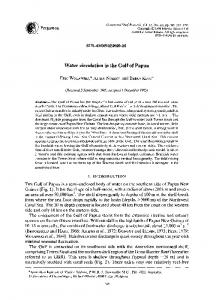
AN E X A M P L E The assembly network used in the example problem is given in Figure 1. The processing times (min) for the elements are given next to the nodes. 4
6
6
Figure 1. Assembly Network for the Example Problem 1. Assembly Line Balancing In this example, a simple heuristic procedure is used for line balancing. The maximum number o f elements per station is limited to three. Therefore, the minimum number o f stations needed is four. The results o f the various station configurations are summarized in Table 1. 2. Parallel Stations The results o f parallel station calculations for a manpower level o f 12 are summarized in Table 2. For example, if 4-station configuration is selected, 3 parallel stations are required for every station type. For a 5-station configuration, the number o f parallel stations would be 3, 2, 3, 2 and 2 for stations 1, 2, 3, 4 and 5, respectively. Among the alternative configurations, 4-station configuration is the one with maximum output rate (9.99 units/hr). This analysis is repeated for all possible manpower levels (from 4 to 30) and the best results are summarized in Table 3.
Alternative Configuration
Stations 1
4 Station 5 Station 6 Station 7 Station 8 Station 9 Station 10 Station I I Station
2
3
4
5
AR
6
!,2,4 3,6,7 5,8 9,10,11 1,2,4 3,7 5,6,9 8 10,11 1,2 3,6 4,5 7,9 8 10,11 1,2 3,6 4,7 5 8 9,10 1,2 3 6,7 5 4,9 8 I 3 2,4 5 6,7 8 I 3 2 4 5 6,7 I 3 2 4 5 6 Table 1. Operation Assignments to Stations
7
8
9
!! 10 I1 9 10 I1 8 9 10 7 8 9 for Alternative
10
!1
units/ hr 3.33 4.00 4.61 5.00 6.00 6.66 11 6.66 I0 11 6.66 Configurations
CT
min 18 15 13 12 10 9 9 9
Selectedpapersfrom the 22ndICC&IEConference
470 Alternative Configuration
Stations I
2
3
4
4 Station 5 Station 6 Station 7 Station 8 Station 9 Station 10 Station I I Station Table 2. Number
3 3 3 3 2 3 2 2 2 2 2 2 2 2 I I 2 2 I 2 I I 1 I o f Parallel Stations
Manpower Level
AR
4 5 6 7 8 9 10 I1 12
Best Conf.
4 5 6 6,7 4 4 5 4,5 4 Table 3. The
3 2 2 I 1 I ! I for
5
7
8
Best Conf.
9
AR
I0
CT
units/ min hr 9.99 6.00 2 8.56 7.00 2 2 9.22 6.50 2 2 1 7.50 8.00 2 2 1 I 7.50 8.00 I 2 1 I 1 7.50 8.00 I I 2 I I I 7.50 8.00 ! I 1 2 I I I 7.50 8.00 Various Configurations for a Manpower Size o f 12 Operators
Manpower Level
6
AR !I
Manpower Level
3.33 4.00 4.62 5.00 6.66 7.04 8.00 8.56 9.99
13 4 10.56 14 5 12.00 15 4,5 12.84 16 4 13.32 17 4 14.08 18 4 15.00 19 4 16.65 20 4,5 17.12 21 6,7 18.00 Summaryo f Best Results for Different Manpower
Best Conf.
AR
22 4 18.75 23 4,5 19.98 24 4 21.12 25 4,5 21.40 26 4 22.50 27 4 23.31 28 4 24.64 29 4 25.68 30 4 26.25 Levels Considered
3. Parallel Lines The example problem is solved for different demand rates and the results are tabulated in Table 4. For example, for a demand rate o f 100 units/hr, 3 line configurations were selected, namely manpower levels 4, 19 and 29. All o f the lines have 4-station configuration. Furthermore, the required number o f lines with manpower level four is 2 and with manpower level 29 is 3. Demand Rate units/hr 10 25 50 60 75 100
Line Configuration I Man. Level
Line Configuration 3
Line Configuration 2
ConK (s)
# of Lines
Man. Level
Con£ (s)
# of Lines
Man. Level
Confi (s)
# of Lines
4
4
2
5
5
1
29 4 4 4
4 4 4 4
1 I 4 I
24 24 24
4 4 4
1 1 1
29 29 29
4 4 4
! 1 2
4
4
2
19
4
I
29
4
3
Table 4. Design o f Assembly Lines for Different Demand Rates In this example problem, the configurations with lower number o f stations resulted in better efficiency and hence assembly rate figures. However, there is a need to do an extensive experimentation to see if these results hold in different problems as well.
REFERENCES [1] Bard, J. "Assembly Line Balancing with Parallel Worksattions and Dead Time," Int'i. J. Prod. Res., Vol. 27, 1989, pp.1005-1018. [2] Pinto, P.A., Dannenbring, D.G. and Khumawala, B.M., " A Branch and Bound Algorithm for A s s e m b l y Line Balancing with Paralleling," Int'l J. Prod. Res., Vol. 19, 1981, pp. 565-576. [3] SUer, G.A. and Dagli, C., A Knowledge-Based System for Selection o f Resource Allocation Rules and Algorithms, in Handbook of Expert System Applications in Manufacturing; Structures and Rules, (eds. A. Mital And S. Anand), Chapman and Hall, 1994, pp. 108-147.