distribution and its relation to permafrost in and around George Lake area, central. Alaska. In the proceedings of ... Throop J. 2010. Thermal state of permafrost in ...
PERMAFROST DISTRIBUTION MAPPING AND TEMPERATURE MODELING ALONG THE ALASKA HIGHWAY CORRIDOR, INTERIOR ALASKA By Santosh K. Panda
RECOMMENDED:
Advisory Committee Chair
Chair, Department of Geology and Geophysics
APPROVED: Dean, College of Natural Science and Mathematics
Dean of the Graduate School
Date
PERMAFROST DISTRIBUTION MAPPING AND TEMPERATURE MODELING ALONG THE ALASKA HIGHWAY CORRIDOR, INTERIOR ALASKA A THESIS
Presented to the Faculty of the University of Alaska Fairbanks
in Partial Fulfillment of the Requirements for the Degree of
DOCTOR OF PHILOSOPHY
By
Santosh K. Panda, M.Sc. Fairbanks, Alaska December 2011
iii
Abstract An up-to-date permafrost distribution map is critical for making engineering decisions during the planning and design of any engineering project in Interior Alaska. I used a combination of empirical-statistical and remote sensing techniques to generate a high-resolution spatially continuous near-surface (< 1.6 m) permafrost map by exploiting the correlative relationships between permafrost and biophysical terrain parameters. A Binary Logistic Regression (BLR) model was used to establish the relationship between vegetation type, aspect-slope and permafrost presence. The logistic coefficients for each variable class obtained from the BLR model were supplied to respective variable classes mapped from remotely sensed data to estimate permafrost probability for every pixel. The BLR model predicts permafrost presence/absence at an accuracy of 88%. Nearsurface permafrost occupies 37% of the total study area. A permafrost map based on the interpretation of airborne electromagnetic (EM) resistivity data shows 22.5 – 43.5% of the total study area as underlain by permafrost. Permafrost distribution statistics from both the maps suggest near-surface permafrost distribution in the study area is sporadic (10 – 50 % of the area underlain by permafrost). Changes in air temperature and/or winter snow depth are important factors responsible for permafrost aggradation or degradation. I evaluated the effects of past and recent (1941-2008) climate changes on permafrost and active-layer dynamics at selected locations using the Geophysical Institute Permafrost Laboratory model. Results revealed that active-layer thickness reached 0.58 and 1.0 m, and mean annual permafrost temperature increased by 1.6 and 1.7 °C during 1966-1994 at two sites in response to increased mean annual air temperature, mean summer air temperature and winter snow depth. The study found that active-layer thickness is not only a function of summer air temperature but also of mean annual air temperature and winter snow depth. Model simulation with a projected (2008-2098) climate scenario predicts 0.22 m loss of near-surface permafrost at one site and complete permafrost disappearance at another site by 2098. The contrasting permafrost behaviors at different sites under similar climate scenarios highlight the role of soil type and ground ice volume on permafrost dynamics; these factors determine permafrost resilience under a warming climate.
iv
Table of Contents Page Signature Page.................................................................................................................i Title Page ........................................................................................................................ ii Abstract .......................................................................................................................... iii Table of Contents ........................................................................................................... iv List of Figures ................................................................................................................ vii List of Tables .................................................................................................................. ix List of Appendices ...........................................................................................................x Acknowledgements ........................................................................................................ xi CHAPTER 1 INTRODUCTION ..................................................................................... 1 1.1. Hypotheses........................................................................................................ 5 1.2. Objectives .......................................................................................................... 5 1.3. Study area ......................................................................................................... 7 1.3.1. Location .................................................................................................. 7 1.3.2. Geologic setting....................................................................................... 7 1.3.3. Vegetation ............................................................................................. 10 1.3.4. Climate .................................................................................................. 10 1.4. Remote sensing as a permafrost mapping tool: a brief review ......................... 11 1.5. Permafrost temperature modeling: a brief review ............................................. 13 1.6. References ...................................................................................................... 16 CHAPTER 2 APPLICATION OF MULTI-SOURCE REMOTE SENSING AND FIELD DATA TO MAPPING PERMAFROST DISTRIBUTION IN INTERIOR ALASKA ............ 25 2.1. Abstract ........................................................................................................... 25 2.2. Introduction ...................................................................................................... 26 2.3. Study area ....................................................................................................... 28 2.4. Methods ........................................................................................................... 29 2.4.1. Field work .............................................................................................. 29 2.4.2. Statistical model .................................................................................... 32
v 2.4.3. Remote sensing inputs .......................................................................... 33 2.4.3.1.
Vegetation mapping ................................................................... 33
2.4.3.2.
Aspect-slope mapping ............................................................... 37
2.4.3.3.
EM resistivity mapping ............................................................... 37
2.4.4. Probabilistic permafrost mapping .......................................................... 40 2.4.5. EM resistivity based permafrost mapping .............................................. 40 2.5. Results ............................................................................................................ 42 2.5.1. Field observations ................................................................................. 42 2.5.2. Statistical permafrost probability modeling............................................. 43 2.5.3. Probabilistic permafrost map ................................................................. 43 2.5.4. EM resistivity based permafrost map ..................................................... 48 2.5.5. Comparison of probabilistic permafrost map with EM resistivity based permafrost map ..................................................................................... 50 2.6. Conclusions ..................................................................................................... 52 2.7. Acknowledgements.......................................................................................... 53 2.8. References ...................................................................................................... 54 Appendices ............................................................................................................. 59 CHAPTER 3 NUMERICAL MODELING OF PERMAFROST DYNAMICS AT SELECTED SITES IN INTERIOR ALASKA .................................................................. 63 3.1. Abstract ........................................................................................................... 63 3.2. Introduction ...................................................................................................... 64 3.3. Study area and site conditions ......................................................................... 66 3.4. Methodology ................................................................................................... 69 3.4.1. Dataset .................................................................................................. 69 3.4.2. Permafrost thermal model ..................................................................... 72 3.4.3. Modeling steps ...................................................................................... 73 3.5. Results and discussions .................................................................................. 76 3.5.1. Tussock station ..................................................................................... 76 3.5.2. Drunken Forest station .......................................................................... 79 3.5.3. Bedrock station...................................................................................... 81
vi 3.5.4. Comparison of permafrost and active-layer dynamics at Tussock and Drunken Forest stations ........................................................................ 82 3.5.5. Modeling permafrost dynamics in the 21st century ................................. 83 3.5.5.1.
Tussock station .......................................................................... 84
3.5.5.2.
Drunken Forest station............................................................... 87
3.6. Conclusions ..................................................................................................... 92 3.7. Acknowledgements.......................................................................................... 93 3.8. References ...................................................................................................... 94 Appendix 3A ........................................................................................................... 99 CHAPTER 4 SUMMARY AND CONCLUSIONS....................................................... 100 4.1. Summary ....................................................................................................... 100 4.2. Conclusions ................................................................................................... 101 4.3. Broader impacts............................................................................................. 103 4.4. Recommendations and scope for future work ................................................ 105 4.5. References .................................................................................................... 108 Appendix A ................................................................................................................. 110 Appendix B ................................................................................................................. 139
vii
List of Figures Page Figure 1.1:
Map of Alaska Highway Corridor ............................................................. 4
Figure 1.2:
Study area map ....................................................................................... 8
Figure 2.1:
Study area map ..................................................................................... 30
Figure 2.2:
Vegetation map ..................................................................................... 35
Figure 2.3:
Schematic layout of data processing and analytical methods ................ 41
Figure 2.4:
Permafrost map ..................................................................................... 46
Figure 2.5:
Resistivity classification map ................................................................. 49
Figure 2.6:
Comparison of resistivity based permafrost map with probabilistic permafrost map ..................................................................................... 51
Figure 2B.1:
Study area map showing different combinations of photo-interpreted permafrost (Reger and Hubbard, 2010) and probabilistic permafrost classes. ................................................................................................. 61
Figure 3.1:
Study area map ..................................................................................... 67
Figure 3.2:
Reconstructed mean annual air temperature, mean summer air temperature and mead annual snow depth at Dry Creek climate station 71
Figure 3.3:
Comparison of measured soil temperature with modeled soil temperature .............................................................................................................. 75
Figure 3.4:
Modeled permafrost dynamics at Tussock Station................................. 78
Figure 3.5:
Modeled permafrost dynamics at Drunken Forest station ...................... 80
Figure 3.6:
Projected climate data at Tussock station.............................................. 85
Figure 3.7:
Modeled permafrost temperature at Tussock station ............................. 86
Figure 3.8:
Corelation of projected mean summer air temperature and active-layer thicknes ................................................................................................. 88
Figure 3.9:
Modeled permafrost dynamics at Drunken Forest station ...................... 89
Figure 3.10:
Projected mean summer (June, July, and August) and winter (December, January, and February) air temperatures from the IPCC five-climatemodel composite ................................................................................... 91
viii Figure A1:
Resistivity variation with temperature for different types of geologic materials.............................................................................................. 111
Figure A2:
A small section of the study area for which airborne resistivity data was processed............................................................................................ 112
Figure A3:
A pseudo-layer half-space model ........................................................ 115
Figure A4:
Raster resistivity image of a part of the study area. ............................. 117
Figure A5:
Comparison of line resistivity with raster resistivity along NW-SE trending profile line of flight line 227 (Red: line data; Blue: raster data). ............ 119
Figure A6:
Comparison of line resistivity with raster resistivity along E-W trending profile line of flight line 109 (Red: line data; Blue: raster data). ............ 121
Figure A7:
Influence of topography and bird height on in-phase and quadrature component of 140000 Hz line data along the flight line 227 ................. 122
Figure A8:
Influence of bird height and topography on in-phase and quadrature component of 140000 Hz frequency line data along flight line 109 ...... 123
Figure A9:
Box plot of raster resistivity values for GSPCs ..................................... 124
Figure A10:
A scatter plot of apparent resistivity versus aspect for each pixel in the study area ........................................................................................... 126
Figure A11:
Box plots (A-O) of apparent resistivity values for different GSPCs in different surficial geologic units............................................................ 128
ix
List of Tables Page Table 2.1:
Summary of field data collected in different vegetation and topographic settings .................................................................................................. 31
Table 2.2:
Vegetation classification accuracy ......................................................... 36
Table 2.3:
Input variables in the BLR model and their coefficients.......................... 38
Table 2.4:
Relationship between resistivity and frozen/ unfrozen ground condition .... .............................................................................................................. 39
Table 2.5:
Classification statistics from BLR model runs with training and testing data ....................................................................................................... 44
Table 2.6:
Classification statistics from BLR model run using all sampled data points .............................................................................................................. 45
Table 2.7:
Vegetation classes and permafrost distribution...................................... 47
Table 2A.1:
BLR model classification accuracy with different input variables ............ 59
Table 3.1:
Vegetation type and soil profiles at three soil temperature data logger stations .................................................................................................. 68
Table 3.2:
Input parameters in the GIPL model ...................................................... 74
Table 3.3:
Calculated average MAAT, MASD, MAPT, ALT, and mean annual soil temperature at three stations under investigation .................................. 77
Table A1:
Survey specifications ........................................................................... 114
x
List of Appendices Page Appendix 2A Empirical-statistical model sensitivity analysis ....................................... 59 Appendix 2B Comparison of probabilistic permafrost map with photo-interpreted map ... .............................................................................................................. 60 Appendix 3A Abbreviations ........................................................................................ 99 Appendix A
Analysis of airborne electromagnetic resistivity data for near-surface permafrost mapping along Alaska Highway corridor, Interior Alaska… 110
Appendix B
Thesis related publications and presentations ..................................... 139
xi
Acknowledgements I would like to thank and acknowledge the help and support that I received from many individuals and organizations in completion of my Ph.D. research. I was fortunate enough to have a Ph.D. committee that cared not only for my work but also for my personal well being and supported me through many ups and downs of my research. I am especially grateful to my adviser Dr. Anupma Prakash for her support, guidance and care that she showered on me throughout these years. She did everything she could have done to make sure that I had a happy life in Fairbanks. I thank my Ph.D. Committee members, Dr. Diana Solie, Mr. Torre Jorgenson, and Dr. Vladimir Romanovsky, from the bottom of my heart for their valuable time, guidance and encouragement. It was an honor to work with them. I would like to thank my funding agencies, the Alaska Division of Geological & Geophysical Surveys, Alaska Space Grant Program, Department of Geology & Geophysics, Geophysical Institute (GI), Center for Global Change and Arctic System Research, and UAF Graduate School for their financial support during this project. Thanks are also due to Dr. Robert J. Henszey, Dr. Catherine L. Hanks, Dr. Gary Holton, Dr. Guido Grosse, and the late Kevin Engle for their financial support in the form of short term jobs when I needed one most. It is always good to have an assistant in the field and I was lucky to have many. I thank all my field assistants for their company and help in the field and for all the fun memories. A big thank you to all the friends that I made at UAF and colleagues for making my life in Fairbanks so memorable. You have been an important part of my social and professional life and a great source of inspiration. I will cherish the time I spent with you for the rest of my life. Last but not the least I would like to thank the staff and faculties of UAF and the GI for their support and services. Thank you for making UAF a great place to study and live.
1
CHAPTER 1 INTRODUCTION Permafrost or perennially frozen ground is defined as “ground (soil or rock and included ice and organic material) that remains at or below 0 °C for at least two consecutive years, for natural climatic reasons” (van Everdingen, 1998). Permafrost and permafrost-affected regions underlie ~22% of the exposed land in the Northern hemisphere (Brown et al., 1997) and ~80% of Alaska (Jorgenson et al., 2008). Permafrost is abundant in the discontinuous zone of central Alaska under present climatic conditions and its presence is strongly influenced by topography and local ecosystem characteristics. Permafrost stability is affected by natural causes, such as rising near-surface air temperature, changes in winter snow thickness, fire, flood etc., and/or anthropogenic causes, such as removal of surface vegetation for land-use or construction of a dam or reservoir. Permafrost is considered degrading if such causes result in decreasing the thickness or the areal extent of permafrost (van Everdingen, 1998). Active-layer is the layer of ground above permafrost that thaws in summer and freezes again in winter (Muller, 1947). It is critical to the ecology and hydrology of permafrost terrain as it provides a rooting zone for plants and acts as a seasonal aquifer for near-surface ground water (Burn, 1998). Its thickness is highly variable and can be anywhere from a few centimeters to a few tens of meters, depending on the local microclimatic condition, thickness of surface organic layer, vegetation type, snow distribution in winter, and local hydrologic condition. Similarly, the amount of ground ice also varies greatly. Permafrost with thin lenses of ice, layered ice, reticulated vein ice and ice wedges as big as 2-4 m long and 3-5 m deep have been reported (French and Shur, 2010). Permafrost degradation has major ecological and engineering implications. The consequences of permafrost degradation can range from local changes in hydrology and vegetation to a potential global increase in the greenhouse gases (Walter et al., 2006; Schuur et al., 2009; Jorgenson et al., 2010). Ice-rich ground is commonly found at the top of permafrost (Mackay, 1983; Burn, 1988) and therefore the melting of ground ice in
2 degrading permafrost may lead to subsidence and accelerated erosion (Mackay, 1970). Degrading permafrost affects surface hydrology by impounding water in subsiding areas and enhancing drainage in upland areas (Woo, 1992). Subsequent changes in soil drainage can change the habitat composition for vegetation and wildlife (Jorgenson and Osterkamp, 2005), alter the soil carbon budget (Schuur et al., 2008), and can result in the emission of green house gases (Turetsky et al., 2007; Christensen et al., 2004). The type of surface material and ground ice content define the nature of permafrost. Understanding the nature and distribution of permafrost is critical for guiding the engineering design of planned infrastructure and for predicting ecological responses to changing permafrost conditions (Brown et al., 1981). For example, improved methods for mapping permafrost distribution are essential to support engineering decisions when planning routes for roads and pipelines and to understand the dynamics of boreal forest ecosystem in Interior Alaska. Ferrians (1965) classified permafrost areas into four classes, depending on the percent of the land area that is underlain by permafrost. The areas are designated as “continuous permafrost” ≥( 90%), “discontinuous permafrost” (50-90%), “sporadic permafrost” (10-50%) and “isolated permafrost” ( 0 was assigned as vegetated. The unvegetated pixels (NDVI < 0) encompassing barren flood plains, landslides, exposed bedrock and manmade structures were excluded from subsequent analyses as these land-covers in the study area are highly likely to be underlain by rocky soils where determination of permafrost is difficult with only hand-held tools. Image texture, defined as the function of the spatial variation in pixel intensities (gray-scale values), was also used as a means for discriminating different vegetation types. For SPOT band 3 we produced a texture map using a variance operator (ERDAS Field Guide, 2008). Analysis of this map shows that different vegetation canopies display different textural characteristics (for example the Mixed Spruce and Deciduous vegetation class shows higher variance values compared to either Spruce or Deciduous vegetation classes; Open Spruce in low-lying valleys shows lower variance compared to Closed Spruce forest on upland areas). Field observations also suggested that vegetation distribution depends on topography (elevation and slope). Therefore, we created an image composite of seven layers which includes bands 3, 2, and 1 from the SPOT scene, the NDVI layer, a texture (variance) layer, and elevation and slope layers from AIRSAR DEM to get the best vegetation classification result. We used the maximum likelihood decision routine in ERDAS Imagine (ERDAS Field Guide, 2008; ESRI Developer Network, 2009) for vegetation classification. This considers both the variances and covariances of the class signatures when assigning each cell to one of the classes represented in the signature file. With the assumption that the distribution of a class sample is normal, a class can be characterized by the mean vector and the covariance matrix. Given these two characteristics for each cell value, the statistical probability is computed for each class to determine the membership of the cells to the class. With equal probabilities for each class defined in the signature file, each cell is assigned to the class to which it has the highest probability of being a member (ERDAS Field Guide, 2008; ESRI Developer Network, 2009). We mapped six vegetation classes from the seven layer image composite with an overall classification accuracy of 86.5% based on training polygons (Figure 2.2 and Table 2.2).
35
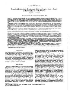
Figure 2.2: Vegetation map. Vegetation map of the study area generated by using the Maximum Likelihood classification algorithm in ERDAS Imagine. White spaces within the vegetation map are masked out areas (water bodies, barren surfaces, clouds and recent burns).
36 Table 2.2: Vegetation classification accuracy. Numbers in parentheses in the first column represent number of sampled stations in that vegetation class. Vegetation
Aspen
Wetland
Mixed
Open
Meadow
Spruce and
Spruce
Class
Aspen (21)
Wetland
Deciduous
Closed
Total
%
Spruce
Correct
Correct
Deciduous
20
1
-
-
-
-
20
95.2
1
14
-
-
-
-
14
93.3
1
1
65
5
-
6
65
83.3
-
-
2
42
-
1
42
93.3
5
1
4
2
14
14
53.8
-
-
7
2
-
96
91.4
251
86.5
Meadow (15)
Mixed Spruce and Deciduous (78)
Open Spruce (45)
Deciduous (26)
Closed
96
Spruce (105)
Total (290)
37 The classification statistics revealed that vegetation covers 81% of the study area. Open Spruce, Closed Spruce, and Mixed Spruce and Deciduous vegetation classes are the dominant vegetation types, representing 82% of the total vegetation cover. 2.4.3.2.
Aspect-slope mapping
The AIRSAR DEM was used to derive the aspect-slope map of the study area using the Spatial Analyst tool in ArcMap 9.3. We reclassified the aspect map into eight aspect classes using 45 degree aspect intervals (Table 2.3). Jorgenson et al. (1999) investigated the permafrost and ecology relationship at Fort Wainwright, Alaska, and found an 8° slope as the frequent boundary between frozen retransported deposits and unfrozen upland loess. This 8° cut-off may also correspond to where slope-wash and rill erosion can shift from erosion to deposition. The deposition of fine-grained soil changes the thermal characteristics and makes the soil more prone to permafrost development. Also, low-lying areas and valley bottoms in Interior Alaska are more likely underlain by near-surface permafrost than upland areas due to the presence of a thicker surface organic layer and winter temperature inversion (Panda et al., 2010). Hence, we extracted all the pixels with slope value less than 8° (which occupy 57% of the study area) from the slope map and added them to the aspect map as a low-lying surface class. 2.4.3.3.
EM resistivity mapping
Frozen clay, silt, peat, sand and gravel show resistivity greater than 60, 60, 300, 300 and 800 Ohm-m, respectively (Hoekstra and McNeill, 1973; Scott and Kay, 1988; Scott et al., 1990). Bedrock is generally highly resistive to electric currents whether frozen or not. Therefore, it is often times difficult to differentiate frozen bedrock from unfrozen bedrock using resistivity data alone. Hence, we excluded all the bedrock areas from the resistivity map using a generalized bedrock map of the study area. We classified the rest of the resistivity map into four classes based on resistivity value ranges for different ground material types presented by Scott and Kay (1988) (Table 2.4).
38 Table 2.3: Input variables in the BLR model and their coefficients. Class
Vegetation
Aspect-slope
Constant
Description
Coefficient
Aspen
Distinct patches of aspen trees
-19.4
Wetland Meadow
Open grass fields in drained lake beds and inactive flood plain
-3.0
Mixed Spruce and Deciduous
Dominantly mixed vegetation type (white spruce, black spruce, and different types of deciduous trees)
0.0
Open Spruce
Scattered, usually short and stunted black spruce found in low-lying valleys and plains
Deciduous
Dominantly one or more types of deciduous vegetation (birch, balsam poplar, dwarf birch, resin birch, alder, aspen etc.)
Closed Spruce
Densely populated spruce trees (white spruce, black spruce or a mix of both)
North
Aspect: (337.51 – 22.50 )
-3.38
North East
Aspect: (22.51 – 67.50)
-0.18
East
Aspect: (67.51- 112.50)
0.82
South East
Aspect: (112.51 – 157.50)
0.43
South
Aspect: (157.51 – 202.50)
-18.63
South West
Aspect: (202.51 – 247.50)
-20.61
West
Aspect: (247.51 – 292.50)
-16.05
North West
Aspect: (292.51 – 337.50)
0.02
Low Lying Plain
Slope < 8°
34.5
-19.65
2.85
0.0 -1.55
39 Table 2.4: Relationship between resistivity and frozen/ unfrozen ground condition. The relationship varies with the material type. Class Resistivity (Ohm-m)
Frozen/ Unfrozen
% of study area
1
< 60
Likely unfrozen irrespective of material type.
2
60 - 800
Frozen if the material type is clay, silt, sand or peat.
21.35
3
800 - 10000
Frozen except in presence of bedrock.
22.50
4
> 10000
Frozen bedrock.
0.02
0.13
40 2.4.4. Probabilistic permafrost mapping We applied the established relationship (in the form of logistic coefficients for each input variable class) to vegetation and aspect-slope classes mapped from remotely sensed data. The Raster Calculator tool in ArcMap 9.3 was used to estimate the permafrost probability for each pixel in two steps. In the first step, we calculated the logodds or Z (Equation (2.2)) for every pixel in the input maps using the coefficients obtained from the BLR model for input variable classes. In the second step, we calculated the probability of permafrost presence by substituting the value of Z in Equation (2.1) (Figure 2.3). For
this study, pixels with probability less than 0.5 are
classified and mapped as devoid of near-surface permafrost (‘permafrost absent’) and pixels with probability greater than 0.5 are classified and mapped as underlain by nearsurface permafrost (‘permafrost present’). 2.4.5. EM resistivity based permafrost distribution mapping We interpreted the classified resistivity map as follows: Resistivity Class 1 (resistivity < 60 Ohm-m) as permafrost absent irrespective of material type; Resistivity Class 2 (resistivity 60-800 Ohm-m) as permafrost present/ absent depending on the material type (for example a pixel with resistivity 200 Ohm-m might be frozen if the material type was silt or clay and might not be frozen if the material type was sand or gravel), but because we did not know the material type in each pixel this class is not as useful as others for permafrost mapping; Resistivity Class 3 (resistivity 800-10000 Ohmm) as permafrost present irrespective of material type because we already excluded the bedrock areas and any other material type with resistivity > 800 Ohm-m should be frozen (Hoekstra and McNeill, 1973; Scott and Kay, 1988; Scott et al., 1990). Resistivity Class 4 (resistivity > 10000 Ohm-m) occupies a tiny fraction (0.1 %) of the study area and most likely maps out the small patches of unexposed bedrock not included in ADGGS generalized bedrock map.
41
Figure 2.3: Schematic layout of data processing and analytical methods. Pixels with probability < 0.5 are classified and mapped as devoid of near-surface permafrost (permafrost absent) and pixels with probability > 0.5 are classified and mapped as underlain by near-surface permafrost (modified after Panda et al., 2010).
42 2.5.
Results
2.5.1. Field observations Analysis of field data showed that vegetation type was strongly related to soilpermafrost characteristics. Vegetation where permafrost was absent (0%) included Aspen, Deciduous and Wetland Meadows (Table 2.1). In contrast, permafrost was found at intermediate frequency in Closed Spruce (78%) and at high frequency in Open Spruce (100%). These values are similar to permafrost frequency for ecosystems within Fort Wainwright in the central Tanana Valley, where frequencies of occurrence were 0% for Upland Moist Broadleaf Forest, 0% for Lowland Fen Meadows, 17% for Upland Moist Needleleaf Forest (white spruce), 84% for Lowland Wet Needleleaf Forest (black spruce), and 100% for Lowland Tussock Bogs (Jorgenson et al., 1999). Vegetation structure alone is not a strong indicator however. For example, permafrost occurrence for Needleleaf forests on Fort Wainwright varied greatly for riverine (0%), upland (17%), lowland gravelly (50%), and lowland (84%) physiographies. Thickness of surface organic layers, including live mosses, was inversely related to active-layer thickness in different vegetation classes. For example, on low-lying plains (slope < 8°) the organic layer was thickest (26 cm) and the active-layer was thinnest (47 cm) for the Open Spruce vegetation class. In Closed Spruce, and Mixed Spruce and Deciduous vegetation classes, organic-layer thicknesses were 20 cm and 13 cm, and the active-layer thicknesses were 60 cm and 70 cm, respectively. The difference in active-layer thickness among vegetation classes was not only due to the difference in organic layer thickness, but may also have been due to the difference in winter snow depths. The winter snow cover, which acts as an insulator and retards the amount of heat flowing out of the ground, is generally shallower in densely populated Closed Spruce vegetation class compared to less dense Mixed Spruce and Deciduous vegetation class, because of the interception and holding of snow by coniferous tree canopies (Viereck, 1970; Sturm et al., 2001; Jorgenson et al., 2000).
43 2.5.2. Statistical permafrost probability modeling To avoid a chance occurrence of anomalous model performance, we ran the BLR model ten times, each time with approximately two-thirds of the randomly selected sampled data to train the model (training data) and the remaining one-third to validate the model (testing data). The minimum and maximum classification accuracies achieved with the training data ranged from 87.3% to 90.6%, while those for testing ranged from 80.8% to 89.5% (Table 2.5). The average overall classification accuracy achieved for training and testing data were 89% and 85%, respectively. For all ten model runs, the significance levels using the Hosmer-Lemeshow goodness-of-fit statistic were well above 0.05, suggesting the models adequately fit the input data. The ten model runs with randomly selected training and testing data validated model performance and stability. We then ran the BLR model with all the sampled data to get the best possible coefficients for input variable classes to generate the permafrost probability map of the study area. The model correctly classified 145 data points out of 169 as permafrost absent and 146 out of 161 data points as underlain by permafrost (Table 2.6). The overall classification accuracy achieved was 88%. 2.5.3. Probabilistic permafrost map The high-resolution, spatially continuous map of near-surface permafrost created through BLR modeling shows 45% of the vegetated area (which corresponds to 37% of the total study area) as underlain by near-surface permafrost (Figure 2.4). The distribution statistics suggest permafrost distribution in the study area is sporadic (10 – 50% of the area underlain by permafrost) instead of discontinuous (50 – 90% of the area underlain by permafrost) as previously reported based on limited borehole temperature measurements (Ferrians, 1998; Jorgenson et al., 2008). Permafrost presence was highly related to vegetation type (Table 2.7). Comparison of permafrost and vegetation maps revealed that 100% of the Open Spruce, 87% of Closed Spruce and 11% of Mixed Spruce and Deciduous vegetation classes are underlain by permafrost, whereas the Aspen, Deciduous and Wetland Meadow vegetation classes are devoid of near-surface permafrost in the study area.
44 Table 2.5: Classification statistics of BLR model runs with training and testing data. Model Run
Training Data (%)
Testing Data (%)
Classification accuracy (%) Training data
Testing data
1
71.2
28.8
87.7
83.2
2
71.8
28.2
88.2
88.2
3
68.8
31.2
89.4
85.4
4
73.9
26.1
87.3
89.5
5
74.2
25.8
89.4
83.5
6
67.9
32.1
90.6
82.1
7
69.7
30.3
88.3
87.0
8
71.5
28.5
88.6
87.2
9
73.0
27.0
90.5
82.0
10
70.0
30.0
90.5
80.8
89.0
85.0
Average Classification Accuracy
45 Table 2.6: Classification statistics from BLR model run using all sampled data points. Observed
Predicted
Correct (%)
No permafrost
Permafrost
No permafrost
145
24
85.8
Permafrost
15
146
90.7
Overall (%)
88.2
46
Figure 2.4: Permafrost map. Permafrost distribution map of study area based on probability threshold of 0.5. The BLR model mapped 45% of the vegetated area (which corresponds to ~37% of the total study area) as underlain by near-surface permafrost. Gaps in the permafrost map indicate masked-out zones not included in the study.
47 Table 2.7: Vegetation classes and permafrost distribution. Percentage of mapped vegetation classes and percentage of each vegetation class underlain by near-surface (< 1.6 m) permafrost in the study area. Vegetation Class Aspen
Vegetation Class (%)
Permafrost (%)
8.1
0.0
34.0
87.0
7.2
0.0
Mixed Spruce and Deciduous
36.3
11.0
Open Spruce
11.4
100.0
3.0
0.0
Closed Spruce Deciduous
Wetland Meadow
48 Since ground sampling was conducted up to a maximum depth of 1.6 m, the permafrost map shows permafrost distribution in the top 1.6 m of the ground surface. We do not rule out the presence of permafrost at lower depth for areas mapped as devoid of permafrost, although, based on our field experience, published literature and limited borehole data, permafrost is usually absent under Deciduous, Aspen and Wetland Meadow vegetation cover in the study area. However, the areas mapped as devoid of permafrost in the Closed Spruce and Mixed Spruce and Deciduous vegetation classes may have permafrost at lower depth, which can be confirmed only by drilling deeper holes in the ground. Absence of permafrost on south-facing slopes and presence on north-facing slopes in favorable vegetation settings makes permafrost mapping easy. However, in flats it can be more problematic due to ground water effects. Also identifying permafrost under spruce forest is difficult in contrasting fluvial, colluvial and glacial deposits. 2.5.4. EM resistivity based permafrost map Classification of the resistivity map into four classes helped to map areas underlain by no permafrost, possible permafrost (depending on the material type) and permafrost (Figure 2.5). After excluding the bedrock areas (which cover 47% of the study area), based on the resistivity values alone 22.5% (Resistivity Class 3) of the study area is underlain by permafrost and 21% (Resistivity Class 2) of the study area is underlain by (possible) permafrost if the ground material type were clay, silt, sand or peat. Since we do not know the material type for every resistivity pixel it cannot be confirmed what percentage of Resistivity Class 2 is underlain by permafrost. The Resistivity Classes 1 and 4 together represent a tiny fraction (0.15%) of the study area with little contribution to the overall permafrost distribution statistics in the study area. Thus, permafrost occupies 22.5 – 43.5 % of the study area based on the interpretation of resistivity data.
49
Figure 2.5: Resistivity classification map. Resistivity map classified into four classes; Resistivity Class 1: No Permafrost; Resistivity Class 2: Possible Permafrost; Resistivity Class 3: Permafrost; Resistivity Class 4: Permafrost. White polygons with black outlines are bedrock polygons (from ADGGS bedrock map) excluded from analysis.
50 2.5.5. Comparison of probabilistic permafrost map with EM resistivity based permafrost map Comparison of the probabilistic permafrost map with the resistivity-based permafrost map revealed that 56% of Resistivity Class 2 and 65% of Resistivity Class 3 are underlain by near-surface permafrost according to the probabilistic permafrost map (Figure 2.6). Resistivity Class 1 and 4 were not included in the comparison because of their negligible representation (0.15% of the study area). The lack of stronger correlation between the probabilistic permafrost map with the resistivity based permafrost map was likely due to the effects of surficial materials. In case of Resistivity Class 2, presence or absence of permafrost depends on the material type and resistivity value within the pixel. It is possible that 56% of the Resistivity Class 2 is underlain by permafrost. In case of Resistivity Class 3 (800 – 10000 Ohm-m), there should be 100% agreement between both permafrost maps since all geologic material types with resistivity greater than 800 Ohm-m, except bedrock, should be frozen (bedrock was already excluded from the resistivity map). However, the 35% disagreement between the probabilistic permafrost map and the resistivity based permafrost map may be due to the glacial moraine or outwash deposits (composed of sediments ranging from clay to boulders) scattered throughout the study area or the presence of unexposed bedrock (not mapped in ADGGS bedrock map) that can be highly resistive to the airborne EM signal even though unfrozen. Nevertheless, based on the interpretation of resistivity data permafrost occupies 22.5 – 43.5% of the study area, which is in agreement with the probabilistic permafrost map that shows 37% of the study area as underlain by near-surface permafrost. The study reveals that EM resistivity data has the potential to detect and map permafrost distribution, but its accuracies can be enhanced if used in conjunction with a map of ground material types. Our interpretation of the efficacy of airborne EM data to mapping permafrost concurs with the findings of others. Kellet et al. (2000) mapped discontinuous permafrost in the Canadian sub-arctic using a combination of airborne and surficial geophysical surveys supported by drilling, sampling and borehole geophysical logging. They used spatial distribution of ground-resistivity values and a resistivity-depth profile derived from an inversion model to characterize the subsurface extent of the permafrost. Their study
51
Figure 2.6: Comparison of resistivity based permafrost map with probabilistic permafrost map. 56% of the Resistivity Class 2 (Possible Permafrost) and 65% of the Resistivity Class 3 (Permafrost) are underlain by permafrost according to the Probabilistic permafrost map. Resistivity Class 1 and 4 are not included in the comparison because of their negligible representation (0.15% of the study area).
52 concluded that airborne EM data provided a simplified and regional pattern of the permafrost distribution with some ambiguity in areas where near-surface variations in electrical conductivity (due to buried landfills and other infrastructure) masked deeper permafrost layers. Ground geophysical surveys and drilling revealed a far more complex picture of permafrost distribution. Preliminary results from the investigation of airborne EM data to map permafrost in the discontinuous zone of Yukon Flats revealed good correlation between high resistivity values and known areas of permafrost (Smith et al., 2010). They found high resistivity values over loess deposits, which are generally less resistive to airborne EM signal, due to high ice content. 2.6.
Conclusions High-resolution, spatially continuous maps of near-surface permafrost can be
generated by developing logistic regression models from limited field data and integrating the logistic models in a GIS framework to predict permafrost distribution from remotely sensed data. Analysis of field data showed strong correlations between vegetation and soil-permafrost characteristics. Vegetation covers 81% of the study area. 45% of the vegetated area (37% of the total study area) is underlain by near-surface permafrost. Interpretation of airborne EM resistivity data shows 22.5 – 43.5 % of the study area as underlain by permafrost. The comparison of permafrost distribution from both maps suggests permafrost distribution in the study area is sporadic instead of discontinuous as previously reported based on limited borehole temperature measurements and ground observations. Based on the correlative relationships between permafrost and surface variables in our study area, the logistic coefficients for surface variables likely can be used to generate probabilistic permafrost maps for other parts of Interior Alaska. The airborne EM resistivity data has the potential to detect and map permafrost distribution, but it is more useful when accompanied by a map of ground material type. The probabilistic permafrost map produced in this study will be useful for planning pipeline or railroad routes and identifying areas for more detailed ground investigations. It also will serve as a baseline map along with the vegetation map to
53 identify areas of permafrost degradation and future changes in vegetation cover and wetland areas. 2.7.
Acknowledgements Field support and partial funding for this research was provided through the
Alaska Division of Geologic and Geophysical Surveys (ADGGS). We acknowledge the additional financial support from the Alaska Space Grant Program (ASGP) and the Center for Global Change and Arctic System Research. The authors acknowledge Dr. Richard D. Reger and De Anne S. P. Stevens for their guidance and help in taking field measurements, Dr. Vladimir Romanovsky for explaining the permafrost characteristics in the study area, and Dr. Ron Barry for help with statistical modeling. Co-authors Dr. Solie and Dr. Prakash helped with field data collection. All the coauthors reviewed the manuscript and provided feedback that helped improve the content and language of the manuscript.
54 2.8.
References
Brown J, Ferrians OJ Jr., Heginbottom JA, Melnikov ES. 1997. Circum-Arctic Map of Permafrost and Ground-Ice Conditions. United States Geological Survey CircumPacific Map Series CP-45. Brown RJE, Johnston GH, Mackay JR, Morgenstern NR, Shilts WW. 1981. Permafrost distribution and terrain characteristics. In Permafrost: Engineering design and construction, Johnston GH. (ed.). John Wiley & Sons: Toronto; 31-72. Christensen TR, Johansson T, Malmer N, A°kerman J, Friborg T, Crill P, Mastepanov M, Svensson B. 2004. Thawing sub-arctic permafrost: effects on vegetation and methane emissions. Geophysical Research Letters 31: L04501. ERDAS Field Guide. 2008. ERDAS, Inc. II: 132-133. ESRI Developer Network. 2009. How maximum likelihood classification works at http://edndoc.esri.com/arcobjects/9.2/NET/shared/geoprocessing/spatial_analyst_too ls/how_maximum_likelihood_classification_works.htm. Last accessed on January 14, 2011. Etzelmuller B, Heggem ESF, Sharkhuu N, Frauenfelder R, Kaab A, Goulden C. 2006. Mountain permafrost distribution modeling using a multi-criteria approach in the Hovsgol area, Northern Mongolia. Permafrost and Periglacial Processes 17: 91-104. Ferrians O. 1998. Permafrost map of Alaska. National Snow and Ice Data Center/World Data Center for Glaciology, Boulder, CO. Frauenfelder R, Allgower B, Haeberli W, Hoelzle M. 1998. Permafrost investigations with GIS – A case study in the Fletschhorn area, Wallis, Swiss Alps. In the proceedings of Seventh International Permafrost Conference, Yellowknife, Canada, 291-295. Goodrich LE. 1982. The influence of snow cover on the ground thermal regime. Canadian Geotechnical Journal 19: 421-432.
55 Hoekstra P. 1978. Electromagnetic methods of mapping shallow permafrost. Geophysics 43: 782-787. Hoekstra P, McNeill D. 1973. Electromagnetic probing of permafrost. In the proceedings of Second International Conference on Permafrost, Yakutsk, USSR, 517-526. Hoekstra P, Sellmann PV, Delaney A. 1975. Ground and airborne resistivity surveys of permafrost near Fairbanks, Alaska. Geophysics 40: 641-656. Hosmer DW, Lemeshow S. 2000. Applied logistic regression. John Wiley & Sons: New York; 375 p. Jensen JR. 2000. Remote sensing of vegetation. In Remote sensing of the environment: An Earth resources perspective. Prentice Hall: New Jersey; 333-378. Jorgenson MT, Kreig RA. 1988. A model for mapping permafrost distribution based on landscape component maps and climatic variables. In the proceedings of Fifth International Permafrost Conference. Trondheim, Norway, 176-182. Jorgenson MT, Osterkamp TE. 2005. Response of boreal ecosystems to varying modes of permafrost degradation. Canadian Journal of Forest Research 35: 2100–2111. Jorgenson MT, Roth JE, Raynolds M, Smith MD, Lentz W, Zusi-cobb A, Racine CH. 1999. An ecological land survey for Fort Wainwright, Alaska. United States Army Cold Regions Research and Engineering Laboratory Report 99-9, Hanover, New Hampshire, 83 p. Jorgenson MT, Roth JE, Schlentner SF, Cater TC. 2000. Ecological land evaluation for the Yukon Training Area on Fort Wainwright, Alaska: Permafrost, Disturbance and Habitat use. United States Army Cold Regions Research and Engineering Laboratory Report, Hanover, New Hampshire, 88 p. Jorgenson MT, Yoshikawa K, Kanevskiy M, Shur Y. 2008. Permafrost characteristics of Alaska. Institute of Northern Engineering, University of Alaska Fairbanks, 1 sheet, scale 1: 7,200,000.
56 Kellet R, Hinnell A, Gamey J, Hodges G. 2000. Mapping discontinuous permafrost in the Canadian sub-arctic using a combination of airborne and surface geophysical surveys, SEG Technical Program Expanded Abstracts: 1351-1354. Kreig RA, Reger RD. 1982. Air-photo analysis and summary of landform soil properties along the route of the Trans-Alaska Pipeline System. Alaska Division of Geological & Geophysical Surveys Geologic Report 66: 149 p. Leverington DW, Duguay CR. 1997. A Neural network method to determine the presence or absence of Permafrost near Mayo, Yukon Territory, Canada. Permafrost and Periglacial Processes 8: 205-215. Morrissey LA, Strong L, Card DH. 1986. Mapping permafrost in the boreal forest with Thematic Mapper satellite data. Photogrammetric Engineering & Remote Sensing 52: 1513-1520. Nguyen T-N, Burn CR, King DJ, Smith SL. 2009. Estimating the extent of near-surface permafrost using remote sensing, Mackenzie Delta, Northwest Territories. Permafrost and Periglacial Processes 20: 141-153. Panda SK, Prakash A, Solie DN. 2008. Remote sensing-based study of vegetation distribution and its relation to permafrost in and around George Lake area, central Alaska. In the proceedings of Ninth International Conference on Permafrost, Fairbanks, Alaska, II: 1357-1362. Panda SK, Prakash A, Solie DN, Romanovsky VE, Jorgenson MT. 2010. Remote sensing and field-based mapping of permafrost distribution along the Alaska Highway corridor, Interior Alaska. Permafrost and Periglacial Processes 21: 271-281. Reger RD, Hubbard TD. 2010. Reconnaissance interpretation of 1978-1983 permafrost, Alaska Highway Corridor, Robertson River to Tetlin Junction, Alaska. Alaska Division of Geological & Geophysical Surveys Preliminary Interpretive Report 2009-6C: 13 p., 4 sheets, scale 1:63,360.
57 Reger RD, Stevens DSP, Solie DN. 2008. Surficial-geologic map, Delta Junction to Dot Lake, Alaska Highway Corridor: Alaska Division of Geological & Geophysical Surveys Preliminary Interpretive Report 2008-3A: 48 p., 2 sheets, scale 1:63,360. Rouse JW, Haas RH, Schell JA, Deering DW. 1974. Monitoring vegetation systems in the Great Plains with ERTS. In the proceedings of Third Earth Resources Technology Satellite-1 Symposium, Greenbelt, Maryland, NASA SP-351: 301-317. Sartorelli AN, French RB. 1981. Electro-magnetic induction methods for mapping permafrost along northern pipeline corridors. In the proceedings of Fourth Canadian Permafrost Conference, Calgary, Canada: 283-295 Schuur EAG, Bockheim J, Canadell JG, Euskirchen E, Field CB, Goryachkin SV, Hagemann S, Kuhry P, Lafleur PM, Lee H, Mazhitova G, Nelson FE, Rinke A, Romanovsky VE, Shiklomanov EN, Tarnocai C, Venevsky S, Vogel JG, Zimov SA. 2008. Vulnerability of permafrost carbon to climate change: implications for the global carbon cycle. Bioscience 58: 701–714. Scott WJ, Kay AE. 1988. Earth resistivities of Canadian soils. Canadian Electrical Association Research Report, Montre´al, Canada. Scott WJ, Sellmann PV, Hunter JA. 1990. Geophysics in the study of permafrost. In Geotechnical and Environmental Geophysics, Ward SH. (ed.). SEG 1, 355-384. Smith MW. 1975. Microclimatic influences on ground temperatures and permafrost distribution, Mackenzies Delta, Northwest Territories. Canadian Journal of Earth Sciences 12: 1421-1438. Smith BD, Walvoord MA, Abraham JD, Cannie JC, Voss CI. 2010. Airborne electromagnetic surveys for baseline permafrost mapping and potential long-term monitoring. Abstract NS31A-1387 presented at 2010 Fall Meeting, AGU, San Francisco, California.
58 Sturm M, McFadden JR, Liston GE, Chapin FS III, Racine CH, Holmgren J. 2001. Snow-shrub interactions in Arctic tundra: A hypothesis with climatic implications. Journal of Climate 14: 336-344. Turetsky MR, Wieder RK, Vitt DH, Evans RJ, Scott KD. 2007. The disappearance of relict permafrost in boreal North America: effects on peatland carbon storage and fluxes. Global Change Biology 13: 1922–1934. van Everdingen RO. 1998. Multi-language glossary of permafrost and related ground ice terms. International Permafrost Association, National Snow and Ice Data Center, University of Colorado, Boulder. Viereck LA. 1970. Forest succession and soil development adjacent to the Chena River in Interior Alaska. Arctic and Alpine Research 2: 1-26. Western Region Climate Center (WRCC). 2005. Alaska Climate Summaries. Available at http://www.wrcc.dri.edu/summary/climsmak.html. Last accessed on April 3, 2011. Woo M. 1990. Consequences of climatic change for hydrology in permafrost zones. Journal of Cold Region Engineering 4: 15–20. Zhang Y. 2002. Problems in the fusion of commercial high-resolution satellite as well as Landsat 7 image and initial solutions. Talk presented at Joint International Symposium on Geospatial Theory, Processing and Applications, Ottawa, Canada. International Archives of Photogrammetry and Remote Sensing 34.
59 Appendices Appendix 2A Empirical-statistical model sensitivity analysis The model was run three times, each time with one of the surface variables as the explanatory variable. The model produced 86%, 60% and 56% classification accuracy with vegetation, aspect-slope and elevation as the only explanatory variable, respectively (Table 2A.1). The model run with different combinations of two out of the three variables produced highest classification accuracy (88%) for the combination of vegetation and aspect-slope variables and lowest classification accuracy (60%) for the combination of aspect-slope and elevation variables. Running the model with all three surface variables as explanatory variables did not improve the classification accuracy achieved with the combination of vegetation and aspect-slope variables. This suggests that elevation was not contributing to the overall classification accuracy. Hence, we used a combination of vegetation and aspect-slope as explanatory variables in the final model. Table 2A.1: BLR model classification accuracy with different input variables. Classification accuracy achieved by running the BLR model successively with a single input variable and different combination of input variables. Variable(s)
Classification Accuracy (%)
Only Elevation
56.1
Only Aspect-slope
59.7
Only Vegetation
86.4
Aspect-slope and Elevation
60.0
Vegetation and Elevation
86.4
Vegetation and Aspect-slope
88.2
Vegetation, Aspect-slope, and Elevation
88.2
60 Appendix 2B Comparison of probabilistic permafrost map with photo-interpreted map To assess the accuracy of the probabilistic permafrost map, we compared our results to the photo-interpreted permafrost map published by the Alaska Division of Geological and Geophysical Surveys (Reger and Hubbard, 2010). The extent of permafrost and ice content for this map was inferred by interpreting ~1:63,360 scale, false-color infrared aerial photographs taken in August 1980. Interpreted proxy data included vegetation, slope, aspect, landforms, soil type, local drainage, and terrain features. They mapped permafrost in the corridor in five different classes: continuously frozen (more than 90% of the area inferred to be underlain by permafrost), discontinuously frozen (50–90% of the area underlain by permafrost), sporadically frozen (10–50% of the area underlain by permafrost), generally unfrozen (0–10% of the area underlain by permafrost), and no permafrost. In the analysis, we compared only their continuously and discontinuously frozen permafrost classes with our probabilistic map because the rest of the classes constituted only 7.4% of the total vegetated area and almost always coincided with our permafrost absent class (Figure 2B.1). There was a 75% agreement on a pixel-by-pixel basis between our probability map and the continuously frozen permafrost area identified by Reger and Hubbard (2010) (Figure 2B.1). To compare the discontinuously frozen permafrost class, we extracted all the pixels that fall within Reger and Hubbard’s (2010) discontinuously frozen permafrost polygons and found out that 60% of them were mapped as underlain by permafrost in our model, which is within the frozen percentage range of 50-90% used by Reger and Hubbard (2010). Hence, we conclude that our model-derived permafrost map agrees with the discontinuously frozen permafrost class of the photo-interpreted map. The 25% disagreement between the interpretation of the continuously frozen class could be due to several reasons. First, our permafrost map represents permafrost in the top 1.6 m of the ground surface whereas the photo-interpreted permafrost map represents permafrost up to a depth of 7.5 m. Second, Reger and Hubbard (2010)
61
Figure 2B.1: Study area map showing different combinations of the photo-interpreted permafrost (Reger and Hubbard, 2010) and probabilistic permafrost classes. ‘Generally unfrozen’ and ‘no permafrost’ classes from the photo-interpreted permafrost map were combined and presented as ‘No Permafrost’ class. The hill shade model derived from AIRSAR DEM is in the background. Gaps in the modeled areas indicate masked-out zones that reveal the hill shade. Shades of red and green represent disagreement and agreement between the photo-interpreted and probabilistic permafrost maps, respectively.
62 mapped permafrost by interpreting vegetation from older false-color infrared air-photos taken in August 1980, whereas, we mapped vegetation from a SPOT 5 scene acquired in July 2003. Third, differences in the resolution of the data sets may have had an impact: we used SPOT 5 pan-sharpened multi-spectral images at 2.5 m spatial resolution and 5 m AIRSAR DEM, whereas Reger and Hubbard (2010) used air photos printed at 1:63,360 scale. Fourth, we excluded alpine vegetation from our analysis because we have very few field measurements of this vegetation class. Finally, both approaches have errors associated with the mental and statistical models used for mapping.
63
CHAPTER 3 NUMERICAL
MODELING
OF
PERMAFROST
DYNAMICS
AT
SELECTED SITES IN INTERIOR ALASKA1 3.1.
Abstract Changes in air temperature and/or winter snow depth are important factors
responsible for permafrost aggradation or degradation in Interior Alaska. To evaluate effects of past and recent (1941-2008) changes in air temperature and winter snow depth on permafrost and active-layer dynamics, we reconstructed permafrost thermal history at three locations using the Geophysical Institute Permafrost Laboratory 2.0 model. Results revealed that active-layer thickness reached 0.58 to 1.0 m and mean annual permafrost temperature increased by 1.6 to 1.7 °C during 1966-1994 at two of three sites in response to increased mean annual air temperature, mean summer air temperature and winter snow depth. We found that the active-layer thickness is not only a function of summer air temperature but also of mean annual air temperature and winter snow depth. Model simulation with a projected (2008-2098) climate scenario predicts 0.22 m loss of near-surface permafrost at one site and complete permafrost disappearance in the top 20 m of the ground surface at another site by the end of the 21st century. Permafrost might have been present at the third site before 1950, but no longer exists at this site. Analyses showed contrasting permafrost behaviors at three sites under similar climate scenarios, primarily due to differences in soil properties and ground ice volume; these factors determine permafrost resilience under a warming climate.
1
Panda SK, Romanovsky VE, Prakash A, Marchenko S. In review. Numerical modeling of permafrost dynamics at selected sites in Interior Alaska. Submitted to Permafrost and Periglacial Processes.
64 3.2.
Introduction The air temperature is increasing in most of the permafrost areas of the Earth,
and this increase is influencing the ground surface temperature. The increasing ground temperature is causing widespread thawing and degradation of permafrost in many parts of the polar Northern Hemisphere (Lachenbruch and Marshall, 1986; Osterkamp and Romanovsky, 1999; Jorgenson et al., 2001; Camill, 2005; Osterkamp, 2005, 2007a, 2007b; Osterkamp et al., 2009; Christiansen et al., 2010; Jorgenson et al., 2010; Lewkowicz, 2010; Romanovsky et al., 2010a, 2010b; Zhao et al., 2010). Consequently, the spatial diversity of permafrost thermal conditions is decreasing over time (Smith et al., 2010). Permafrost degradation can bring dramatic changes to landscape features, ecosystem structure, and infrastructure stability. If the recent trend in climate warming continues, its effects on the permafrost thermal regime will be far-reaching, leading to considerable impacts on existing ecosystem structure, ecosystem services, and socioeconomic conditions. In order to minimize the negative impacts of permafrost degradation on ecosystems and society, it is imperative to monitor permafrost dynamics for timely assessment and prediction of possible negative consequences (Romanovsky et al., 2002). The permafrost surface is separated from the direct effects of air temperature by the surface organic layer, winter snow, and the active-layer. These biophysical factors buffer the direct effect of changes in air temperature on permafrost. The surface organic layer, which includes surface vegetation cover and dead organic matter, insulates the ground from warmer summer air temperature, reducing the heat flow from the warmer atmosphere into the colder ground. In winter, when the surface organic layer is frozen, heat flows from the warmer ground into the colder atmosphere. Snow cover insulates the ground from colder air temperature during winter. In the beginning of the thawing season, because of its high latent heat of fusion, snow acts as a heat sink which retards warming of the ground surface. However, the net effect of snow cover causes an increase in the mean annual ground surface temperature (MAGST) (Osterkamp, 2007b). Thawed and frozen thermal properties and the water content of the active-layer significantly influence the warming effect of snow cover (Lachenbruch, 1959; Romanovsky, 1987). The difference in the thermal conductivity of a thawed vs. a frozen
65 active-layer causes a negative ‘thermal offset’, defined as the difference between the mean annual permafrost surface temperature (MAPST) and MAGST (Kudryavtzev et al., 1974; Goodrich, 1978; Burn and Smith, 1988; Romanovsky and Osterkamp, 1995). Consequently, the mean annual ground temperature usually decreases with depth in the active-layer. There are other factors that can also contribute to an increase or decrease of active-layer and permafrost temperatures. Examples include topography (slope, aspect, elevation), surface and subsurface hydrology, geology (soil and rock type, tectonic setting), and natural (fire and flood) and anthropogenic disturbances. However, numerous studies have shown that increases in mean annual air temperature (MAAT), winter snow depth, and a combination of these two factors are the primary causes of permafrost warming and subsequent thawing on local as well as regional scales (Lachenbruch and Marshall, 1986; Osterkamp and Romanovsky, 1996; Osterkamp and Romanovsky, 1999; Jorgenson et al., 2001; Camill, 2005; Osterkamp, 2005, 2007a, 2007b; Osterkamp and Jorgenson, 2006; Åkerman and Johansson, 2008; Romanovsky et al., 2010a). Wendler and Shulski (2009) reported an increase in the MAAT of Interior Alaska by 1.4 °C over the past century compared to 0.8 °C worldwide. The increase in the MAAT of Interior Alaska was not uniform during the past century, being most dramatic during the past three decades. After the end of the ‘Little Ice Age’ in the middle of the 20th century, air temperature warmed until about 1940, followed by a cooling trend until the mid-1970s. In 1976, the shift in Pacific Decadal Oscillation (PDO, a pattern of Pacific climate variability) caused an abrupt 1-2 °C increase in MAAT (Hartmann and Wendler, 2003; Hartmann and Wendler, 2005). The 1980s were the warmest of the 20th century. A cooling trend then developed until the late 1990s, followed by warming again in the beginning of the 21st century. It is anticipated that the recent climate warming will continue into the future with some possible short-term cooling at the inter-annual scale (NRC, 2002; IPCC, 2007). The permafrost table will deepen, mean annual permafrost temperature (MAPT) will increase significantly, and long term permafrost thaw may start in many parts of Interior
66 Alaska (Marchenko et al., 2008). However, there will be regional and local differences in the response of permafrost to warming climate because the buffering effect of surface biophysical factors varies spatially. In this paper, we investigate the influence of temporal changes in near-surface air temperature and snow depth on permafrost dynamics at selected sites in Interior Alaska. The objectives of this paper are to reconstruct the past and recent (1941-2008) thermal history of permafrost by using the Geophysical Institute Permafrost Laboratory (GIPL)
2.0
numerical
model
and
permafrost
temperature
reanalysis
method
(Romanovsky et al., 2002); to evaluate the effects of past and recent climate (change in air temperature and winter snow depth) on permafrost temperature and active-layer thickness (ALT) dynamics at three different ecological and geological settings in Interior Alaska; to compare the permafrost and active-layer dynamics at these three sites that experience similar climatic conditions; and to predict the possible changes in permafrost and active-layer dynamics by using future climate scenarios for the state of Alaska (i.e. monthly air temperature and precipitation for the period 2008-2098) from the Intergovernmental Panel on Climate Change (IPCC) Global Circulation five-modelcomposite A1B (midrange) scenario as input to the GIPL 2.0 model. 3.3.
Study area and site conditions The study area is a section of the Alaska Highway corridor (Figure 3.1). It is the
only land transportation route that connects Alaska with the contiguous US and is the locus of many planned and proposed development projects (e.g. a natural gas pipeline and a railroad) in Interior Alaska. We installed HOBO automatic soil temperature data loggers (Onset, 2010) in three different geological and ecological settings (Table 3.1) along the Alaska Highway corridor. Based on the site characteristics that uniquely represent each station under investigation, in the rest of this document Station 1, Station 2 and Station 3 are referred to as ‘Tussock station’, ‘Drunken Forest station’, and ‘Bedrock station’, respectively. Station 1, Tussock station, is located near Alaska Highway mile post 1393 (28 miles southeast of Delta Junction), approximately 2 km south of the Alaska Highway in a
67
Figure 3.1: Study area map. (A) Location of the study area within Alaska is shown with a white box. (B) Locations of three soil temperature data logger stations (1, 2, and 3) and the Dry Creek climate station along the Alaska Highway. The Alaska Highway (which runs NW – SE) meets the Richardson Highway (which runs N-S) at Delta Junction. The background is a hill shade model derived from the National Elevation Dataset (NED) 60 m Digital Elevation Model.
68 Table 3.1: Vegetation type and soil profiles at three soil temperature data logger stations. Station 1
Station 2
Station 3
(Tussock station)
(Drunken Forest station)
(Bedrock station)
Stunted black spruce (height < 3 m), tussocky ground
Black spruce (height 4-10 m), drunken forest
Predominantly spruce (height 4-10 m) with few willow and birch
Foothill
Mound slope
0.00 – 0.13 m: Moss and grass 0.13 – 0.60 m: Organic silt 0.60 – 2.00 m: Silt 2.00 – 5.00 m: Sand 5.00 – 20.00 m: Gravel
0.00 – 0.20 m: Moss 0.20 – 0.60 m: Organic silt 0.60 – 1.50 m: Sand 1.50 – 20.0 m: Gravel
0.00 – 0.16 m: Moss 0.16 – 0.51 m: Sand 0.51 – 0.87 m: Gruss 0.87 – 1.50 m: Weathered Granite 1.50 - 20.0 m: Granite
Measured active-layer thickness
0.5 m (on 9/29/2007)
0.45 m (on 7/21/2007)
No active layer Hit rock at 0.87 m
Data logger depth
0.5 m
0.45 m
0.87 m
Vegetation
Topography Low plain
Soil profile
Note: Soil profiles are inferred from nearby Department of Transportation and Public Facilities borehole records (Brazo, 1987).
69 tussocky setting (Figure 3.1). It is an open stunted black spruce forest with grass and moss on the surface. Reger et al. (2008) mapped the surficial deposit at this site as stream-terrace alluvium chiefly composed of organic sandy silt and silty sand overlying well-sorted, polymictic sand and gravel. Station 2, Drunken Forest station, is located near Alaska Highway mile post 1370 (52 miles southeast of Delta Junction), approximately 0.18 km south of the Highway in a drunken spruce forest setting. Drunken forest is a common term used to describe trees displaced from their normal vertical alignment due to frost heaving or the melting of subsurface ice wedges that occurs in a permafrost environment. Reger et al. (2008) mapped the surficial deposit as mixed colluvium and alluvial deposits chiefly composed of organic silt mixed with sandy angular to subangular pebble gravels derived from weathered granitic uplands. Station 3, Bedrock station, is located 0.04 km north of Station 2 on the east-sloping face of a small mound. Vegetation is predominantly spruce with some willow and birch. Reger et al. (2008) mapped the site as thinly-buried bedrock. 3.4.
Methodology
3.4.1. Dataset We used HOBO Pro V2 automatic soil temperature data loggers to collect soil temperature data. These data loggers have two sensors; one sensor was placed within the surface organic layer and the other at depth within the soil (Table 3.1). The loggers have been continuously recording data at two-hour intervals since July 2007. The HOBO Pro V2 logger uses an optical USB communications interface (via a compatible shuttle or base station) for launching and reading out the logger and operates in the temperature range of -40 °C to 100 °C (accuracy: 0.25-0.20 °C over -10 to 40 °C) (Onset, 2010). We also collected data on vegetation type, surface organic layer thickness, and winter snow depth at two sites, and soil type and moisture at all three sites. We obtained historic climate data (daily air temperature and precipitation) for the period 1996-2009 from the Dry Creek climate station, which is a National Climate Data Center (NCDC) climate station located at latitude 63.41° N, longitude 144.36° W
70 (elevation 411.5 m asl) approximately 54 km from the Tussock station and 32 km from the Drunken Forest and Bedrock stations. Wendler and Shulski (2009) compared the air temperature data from Fairbanks with data from four other Interior Alaska meteorological stations (Bettles, Galena, McGrath, and Tanana) for the period 1942-2006. They found that the air temperature fluctuation in the last six decades has been uniform in Interior Alaska. Hence, to study permafrost and active-layer dynamics at our three stations, we reconstructed historic (1941-2008) climate data (daily average air temperature and snow depth) for the Dry Creek climate station by deriving a set of linear regression equations (Equation 3.1 and 3.2) based on 13 years of recorded climate data (1996-2009) from the Dry Creek and Fairbanks climate stations. Dry Creek at = 0.93*Fairbanks at – 0.74
R2 = 0.94
(3.1)
Dry Creek sd = 0.91*Fairbanks sd + 0.01
R2 = 0.91
(3.2)
where
at
is daily average air temperature and
sd
is daily average snow depth.
The timing of snow appearance in the beginning of winter, the thickness of snow cover throughout the winter, the duration of snow on the ground, and the timing of snow disappearance in spring change from year to year. All the above factors affect MAGST and, hence, MAPT. However, using all the above factors to study the effect of snow on MAPT for a longer time period would make interpretation complex and results perhaps misleading. Therefore, we decided to use a simpler and more consistent snow parameter to study the effect of changing snow on MAPT; we chose a single snow parameter, mean annual snow depth (MASD), which is the sum of daily snow depth on the ground (for one year) divided by 365 days, to study the effects of changing snow on MAGST and MAPT. A linear trend fit to the Dry Creek MAAT and mean summer air temperature (MSAT) data showed a 1.6 °C rise in both MAAT (from -4.2 °C to -2.6 °C) and MSAT (from 12.5 °C to 14.1 °C) between 1941 and 2008 (Figure 3.2A and 3.2B). However, the linear trend fit to the MASD data for the same time period showed no statistically-
71
Figure 3.2: Reconstructed mean annual air temperature, mean summer air temperature and mean annual snow depth at Dry Creek climate station. (A) Mean annual air temperature obtained by applying regression equation 3.1 on Fairbanks daily air temperature data; the dashed line is linear trend fit to the data. (B) Mean summer air temperature calculated from June, July, and August daily air temperature; the dashed line is linear trend fit to the data. (C) Mean annual snow depth obtained by applying regression equation 3.2 on Fairbanks daily snow depth data.
72 significant trend and an average value of 0.18 m. The MASD was abnormally high (≈0.2 m higher than the average MASD of 1941-2008) in 1970, 1990, and 1992 (Figure 3.2C). The MASD during most of the late 1990s and 2000s was mostly below the average MASD (0.18 m) of 1941-2008. 3.4.2. Permafrost thermal model The GIPL 2.0 model takes air temperature, snow depth, surface organic layer properties, moisture, thermal conductivity and heat capacity of different soil layers as input and simulates daily average soil temperature at desired depths. It is a numerical simulator of the transient temporal and spatial response of permafrost to measured or projected changes in air temperature and snow depth. It numerically solves a onedimensional nonlinear heat equation with phase change. In this model the process of soil freezing/thawing is modeled in accordance with the unfrozen water content curve and soil thermal properties, which are specific for each soil layer and for each geographic location (Marchenko et al., 2008). The mathematical model behind the GIPL 2.0 is the enthalpy formulation of the one-dimensional Stefan Problem (Alexiades and Solomon, 1993; Verdi, 1994). It uses the quasi-linear heat conduction equation, which expresses the energy conservation law:
∂H ( y, t ) = div(λ ( y, t )∇t ( y,τ )), y ∈ Ω,τ ∈ Ψ ∂τ
(3.3)
where H(y, t) is the enthalpy: t
H ( y, t ) = ∫ C ( y, t )dt + Lφ ( y, t ) 0
(3.4)
where: t = Temperature (°C) y = Depth (m); the computational depth domain is 0≤Ω≤20 for our simulation = Time: ψ is the time interval with an initial time step of 24 hours
73 The value of the temperature gradient at the lower boundary (20 m depth) is 0.001 Kelvin/meter. C(y, t) is the heat capacity, L is the latent heat of freezing/fusion, λ(y, t) is thermal conductivity, and Ø(y, t) is the volumetric unfrozen water content. More details of this model are documented by Nicolsky et al. (2007) and Marchenko et al. (2008). 3.4.3. Modeling steps One year of climate data (daily air temperature and snow depth from the Dry Creek climate station) and the initial soil temperature from the installed temperature data logger were supplied as input to the model for model calibration against measured changes in soil temperature. The soil characterizations used in the model (Table 3.2) were based on extensive empirical observations conducted by the Geophysical Institute Permafrost Group at locations representative of the major physiographic units in Alaska. The model parameters were systematically adjusted in successive model runs to achieve a good match between measured and modeled soil temperature at logger depth (Figure 3.3A and 3.3B). Then, the available climate data (1996-2008) from the Dry Creek climate station (daily average air temperature and snow depth) were used in the calibrated model to simulate daily average soil temperature in the upper 20 m of the soil column from 1996-2008. To study permafrost dynamics for a longer period, 68 years of climate data (1941-2008) from Fairbanks were used to reconstruct the climate history of the Dry Creek climate station using a set of linear regression equations (Equations 3.1 and 3.2). The reconstructed climate data for the Dry Creek climate station were used in the model to simulate soil temperature and to analyze the permafrost temperature and active-layer dynamics over the past 68 years.
74 Table 3.2: Input parameters in the GIPL model. Soil and surface organic layer parameters used in the GIPL model for simulating soil and/or permafrost temperature in the upper 20 m of the ground surface. Soil Layer (m)
Moisture (fraction of 1)
Thawed Heat Capacity
Frozen Heat Capacity
Ratio of Frozen to Thawed Thermal Conductivity
0.00 – 0.13 (Moss)
0.92
2.0 X10⁶
1.85 X10⁶
6.6
0.13 – 0.60 (Organic silt)
0.85
2.1 X10⁶
2.00 X10⁶
2.8
0.60 – 2.00 (Silt)
0.52
2.1 X10⁶
1.76 X10⁶
1.3
2.00 – 5.00 (Sand)
0.28
2.5 X10⁶
2.00 X10⁶
1.5
5.00 – 20.0 (Gravel)
0.22
2.4 X10⁶
1.90 X10⁶
1.4
0.00 – 0.20 (Moss)
0.15
1.7 X10⁶
1.50 X10⁶
1.6
0.20 – 0.60 (Organic silt)
0.50
2.6 X10⁶
2.40 X10⁶
1.5
0.60 – 1.50 (Sand)
0.45
2.6 X10⁶
2.00 X10⁶
1.5
1.50 – 20.0 (Gravel)
0.10
2.6 X10⁶
2.00 X10⁶
1.3
0.00 – 0.16 (Moss)
0.03
1.7 X10⁶
1.50 X10⁶
1.3
0.16 – 0.51 (Sand)
0.30
2.6 X10⁶
2.40 X10⁶
1.9
0.51 – 0.87 (Gruss)
0.12
2.6 X10⁶
2.00 X10⁶
1.5
0.87 – 1.50 (Weathered rock)
0.05
2.6 X10⁶
2.00X10⁶
1.2
1.50 – 20.0 (Bedrock)
0.04
2.6 X10⁶
2.00X10⁶
1.3
Tussock station
Drunken Forest station
Bedrock station
Moisture: Volumetric water content as a fraction of 1 Thawed and frozen volumetric heat capacity in J/m3K [J: Joules; m: meter; K: Kelvin] Thawed and frozen thermal conductivity in W/mK [W: Watts; m: meter; K: Kelvin]
75
Figure 3.3: Comparison of measured soil temperature with modeled soil temperature. (A) At Tussock station at 0.5 m depth. (B) At Drunken Forest station at 0.45 m depth; the sharp rise in measured soil temperature during spring is due to the percolation of surface snow melt water to the data logger at depth.
76 3.5.
Results and discussions
3.5.1. Tussock station The MAAT generally decreased during the time period 1941-1965 with an interannual variation as large as 3.2 °C and an average of -4.1 °C (Figure 3.2A and Table 3.3). Unlike MAAT, the MASD during 1941-1965 was more or less stable with an interannual variation as large as 0.15 m and an average of 0.22 m. In response to decreasing MAAT, the permafrost temperature (at 1 m depth) decreased during this time period and was coldest in 1963 (-3.8 °C) due to the combined effect of low MAAT (-4.8 °C) and low MASD (0.17 m). Since 1966 the MAAT has gradually increased; the average MAAT in the period 1966-1994 was -3.0 °C (1.0 °C warmer than in 1941-1965), with an interannual variation as large as 3.1 °C (Figure 3.2A and Table 3.3). The average MASD in 1966-1994 was 0.26 m (0.04 m higher than in 1941-1965), while in 1990 and 1992 the MASD was more than 50% higher than the average 1966-1994 MASD. In response to higher MAAT and MASD, the permafrost temperature also increased, from -2.5 °C to -0.9 °C using a linear trend fit, and the average MAPT was -1.7 °C, which is 0.9 °C higher than the average MAPT from 1941-1965 (Figure 3.4A and Table 3.3). The ALT gradually increased from 0.45 m to 0.58 m starting in 1966; it was thickest (0.58 m thick) in 1992-93 and 1995 (Figure 3.4B). Increases in MAAT, MASD, and MSAT (from 13.5 °C to 14.0 °C) during 1966-1994 resulted in gradual thickening of the active-layer. The ALT increased rapidly during 1989-1994 and was thickest during this period. Comparing the average 1989-1994 MSAT with that of 1983-1988 (the 6-year period before 1989) and 1995-2000 (the 6-year period after 1994) revealed that the average 1989-1994 MSAT was 0.4 °C and 0.7 °C higher than that of the 1983-1988 and 1995-2000 periods, respectively. The MASD in 1989-1994 was 0.11 m and 0.13 m higher than that of the 1983-88 and 1995-2000 periods, respectively.
77 Table 3.3: Calculated average MAAT, MASD, MAPT, ALT, and mean annual soil temperature at three stations under investigation. Station
1941-1965
1966 - 1994
1995 - 2008
All three stations
Average MAAT
-4.1 °C
-3.0 °C
-3.0 °C
Tussock station
Average MASD
0.22 m
0.26 m
0.20 m
Average MAPT at 1 m depth
-2.6 °C
-1.7 °C
-2.0 °C
ALT range
0.38 – 0.47 m
0.43 – 0.58 m
0.45 – 0.58 m
Average MASD
0.17 m
0.20 m
0.15 m
Average MAPT at 1 m depth
-1.9 °C
-0.85 °C
-0.8 °C
ALT range
0.37 – 0.54 m
0.45 – 0.99 m
0.52 – 1.0 m
Average MASD
0.17 m
0.20 m
0.15 m
Average mean annual soil temperature at 1 m depth
0.7 °C
1.9 °C
1.4 °C
Drunken Forest station
Bedrock station
Note: The daily snow cover at Tussock station was adjusted (by adding 0.1 m to daily snow depth data from Dry Creek climate station) to account for the effect of rough surface topography and open forest canopy which favors more snow accumulation on the ground compared to sites with relatively smooth surfaces and dense forest canopy (Viereck, 1970; Sturm et al., 2001; Jorgenson et al., 2000).
78
Figure 3.4: Modeled permafrost dynamics at Tussock station. Modeled mean annual permafrost temperature and active-layer thickness for the time periods 1941-2008 and 1965-2008 (with 20% less daily snow depth) obtained from the calibrated GIPL model. (A) Permafrost temperature (at 1 m depth). (B) Active-layer thickness.
79 Model simulation with decreased snow showed that a 20% decrease in daily winter snow depth could cause up to 1.6 °C decrease in MAPT and up to 0.10 m decrease in ALT at this station depending on the snow density, seasonal air temperature, soil moisture, and soil active- layer thermal properties (Figure 3.4). Hence, both higher summer air temperature and deeper winter snow depth were responsible for the rapid increase in ALT during 1989-1994. Since the winter of 1995-96 was not cold enough to balance the warming effect of increased snow in previous years, the active layer continued to be thickest in 1995 (Figure 3.4B). The average MAAT and MSAT in 1995-2008 were the same as in 1966-1994; however, the average MASD was 0.20 m (0.06 m less than the average MASD in 1966-1994). The average MAPT in 1995-2008 was -2.0 °C (0.3 °C lower than the average MAPT in 1966-1994). Hence, during 19952008 the decrease in MASD was the principal cause of the decrease in MAPT at this station. The ALT also decreased in 1996-2008; the average ALT in this period was 0.10 m less than in 1992-93. These findings are in disagreement with the implicit assumption that ALT is a function of summer air temperature only and suggest that MAAT and winter snow depth may have a strong influence on the ALT, since the depth to which ground thaws in summer and freezes in winter is ultimately a function of balance between summer and winter energy fluxes at the ground surface. In response to wide-ranging interannual variations in MAAT and MASD, MAPT (at the 1 m depth) also varied widely with an interannual fluctuation as large as 1.9 °C (Figure 3.4A). This demonstrates the very dynamic response of the near-surface permafrost to changing MAAT and MASD at this station. The near-surface air temperature and near-surface permafrost temperature vary in tandem, and an increase or decrease in snow cover can accelerate or decelerate the effect of increasing air temperature on permafrost. 3.5.2. Drunken Forest station Like at Tussock station, MAPT at this station (at the 1 m depth) decreased during the time period 1941-1965 in response to decreasing MAAT (Figure 3.5A). The
80
Figure 3.5: Modeled permafrost dynamics at Drunken Forest station. Modeled mean annual permafrost temperature and active-layer thickness for the time periods 19412008 and 1965-2008 (with 20% less daily snow depth) obtained from the calibrated GIPL model. (A) Permafrost temperature (at 1 m depth). (B) Active-layer thickness.
81 MAPT was coldest in 1963 (-2.8 °C) due to the combined effect of low MAAT (-4.8 °C) and low MASD (0.11 m). In response to increasing MAAT and MASD in 1966-1994, the MAPT increased (from -1.7 °C to -0.01 °C using a linear trend fit); the average MAPT was -0.9 °C (0.9 °C higher than the average MAPT in 1941-1965) (Figure 3.5A). The ALT has gradually increased since 1966 (from 0.45 m – 1.0 m) and was thickest (1.0 m thick) in 1995 due to increases in MAAT, MASD, and MAST (Figure 3.5B). The effect of abnormally high snow depth in 1990 and 1992 was more dramatic at this station than it was at Tussock station. Model simulation with 20% decrease in daily winter snow depth showed up to 1.0 °C decrease in MAPT and up to 0.31 m decrease in ALT at this station depending on the snow density, seasonal air temperatures, soil moisture, and soil thermal properties in the active layer (Figure 3.5). Hence, the modeling results suggest that winter snow depth played a major role in the rapid ALT increase during 1989-1995 that occurred along with a 0.4 °C increase in average MSAT. The warming effect of high snow depth increased not only the ALT but also the soil temperature in the active-layer to such an extent that the active layer did not refreeze completely for the following three winters, resulting in the development of a short-lived talik that lasted from 1992-1994 before it disappeared in 1995. Snow depth was also abnormally high in 1970 but the model did not show any talik development in 1970 because MAPT was colder (-1.0 °C), perhaps reflecting the fact that several years of high snow depth are required under present climatic conditions to cause the substantial change in soil temperature required to develop a talik. In the future warmingclimate scenario predicted by climate models, such short-term taliks will continue to appear and disappear until the climate has warmed enough so that the winter temperature will no longer be able to freeze the entire active layer, resulting in a permanent talik at this station. 3.5.3. Bedrock station This station is located just 40 m north of the Drunken Forest station on the eastfacing slope of a small mound, but the surface geology at this station contrasts starkly with that at the Drunken Forest station. During soil temperature data logger installation,
82 we hit granite bedrock at less than one meter depth. The bedrock was overlain by gruss (weathered granite), with sand uppermost. We modeled this station by assuming permafrost was present here in the early 1940s. However, the modeling result revealed that permafrost disappeared in the beginning of the 1950s and never recovered after that. The presence of little or no moisture in bedrock means that the latent heat effect of moisture is minimal, and bedrock is highly responsive to the warming and cooling effect of near-surface air temperature and change in snow depth. Hence, the presence of nearsurface bedrock at a site creates a situation of extremely dynamic ground thermal regime. 3.5.4. Comparison of permafrost and active-layer dynamics at Tussock and Drunken Forest stations Permafrost (at the 1 m depth) at Drunken Forest station in the period 1941-2008 was 0.9 °C warmer than at Tussock station (Table 3.3). According to linear trend fit (statistically significant at the 99% confidence interval), the MAPT at Tussock and Drunken Forest stations increased by 1.6 °C and 1.7 °C respectively during 1966-1994 (the MAPT was highest at both stations in 1994) (Figure 3.4A and 3.5A). However, the magnitude of interannual variation in MAPT was larger at Tussock station than it was at Drunken Forest station. The ALT increased by 0.13 m at Tussock station compared to 0.55 m at Drunken Forest station during 1966-1995 (Figure 3.4B and 3.5B). Since similar climatic conditions (daily air temperature and snow depth) were used for model simulation at both stations, the differences in the behavior of permafrost temperature (the difference in the magnitude of interannual MAPT variability) and ALT at these two stations are attributed to differences in surface organic layer thickness, moisture contents, the amount of ground ice, and the thermal properties of soil layers. The moisture content in organic silt layers below the moss layers are 85% and 50% for the Tussock station and Drunken Forest station, respectively (Table 3.2). The presence of more ground ice in the activelayer helps to propagate the climate signal to greater depth; at the same time, it also slows the active-layer thawing process during summer (due to the latent heat effect of ground ice). The average MSAT in 1996-2008 was 0.4 °C cooler than in 1982-1994. The average MASDs were 0.08 m less in 1996-2008 than they were in 1982-1994 at both
83 Tussock station and Drunken Forest station. The combined effect of cooler MSAT and lower MASD led to a decrease in ALT during 1996-2008 at both stations. The 1.5 °C and 1.0 °C cooler MAAT and MSAT of 1996 (compared to the average MAAT and MSAT temperatures in 1982-1994) and relatively thinner winter snow depth explain the abrupt decrease of 0.07 m and 0.33 m in ALT at Tussock station and Drunken Forest station, respectively, in 1996 (Figure 3.4B and 3.5B). The modeling results showed that permafrost temperature is more sensitive to climate change at Tussock station than at Drunken Forest station; this, in turn, suggests a greater role of surface organic layer thickness, moisture content, ground ice, and soil thermal properties in influencing the response of permafrost to climate change. The presence of a thinner surface organic layer, more ground ice, and colder MAPT at Tussock station than at Drunken Forest station allows better propagation of the climate signal to deeper soil, and hence greater variation in the interannual permafrost temperature at Tussock station. The resilience or vulnerability of permafrost to climate change is controlled to a large degree by the volume and structure of ground ice within the soil (Jorgenson et al., 2010). The colder MAPT also resulted from greater thermal offset (the difference between MAPT and MAGST). Thermal offset can protect permafrost from a warming climate for several tens of years, but in the long run the warming effect will overcome the negative feedback of thermal offset and permafrost will begin to thaw. Hence, the greater volume of ground ice makes the permafrost at Tussock station more resilient to climate change than the permafrost at Drunken Forest station. 3.5.5. Modeling permafrost dynamics in the 21st century We used projected climate data (average monthly air temperature and total monthly precipitation) for Tussock station and Drunken Forest station from the IPCC five-climate-model composite A1B (midrange emission scenario) (available from Scenario Network for Alaska Planning [SNAP] at www.snap.uaf.edu/downloads/alaskaclimate-datasets) to study the possible response of permafrost temperature and ALT to projected changes in 21st century climate.
84 The IPCC five-climate-model composite contains the mean values of average monthly air temperature (ºC) and total monthly precipitation (mm) from the output of the five best models (out of 15 models used by the IPCC) for the state of Alaska, downscaled to 2 km grid cells. The ranks of the models for overall accuracy in Alaska and the far north are as follows: 1) ECHAM5, 2) GFDL21, 3) MIROC, 4) HAD, and 5) CCCMA (SNAP, 2009). 3.5.5.1. Tussock station The projected MAAT shows a cooling trend until 2019, when a warming begins. The air temperature is projected to hover around 0 °C during most of the 2040s, cool down by 1-2 °C during the 2050s, then follow a gradual warming trend and remain above 0 °C for rest of the 21st century (Figure 3.6A). The projected MASD data show a very gentle increase, with MASD ranging from 0.12 m in the beginning of the century to 0.13 m toward the end of the century (Figure 3.6B). The average projected MASD for the time period 2008-2098 is 0.125 m. The modeling results predict that MAPT will decrease by 0.7 – 1.0 °C at Tussock station (at the 1 m, 5 m, and 20 m depths) from 2008-2019 because of a projected cooling trend in MAAT and decrease in MASD. In the early 2020s the MAPT will begin to rise; following a warming trend, it is projected to increase by 1.9 °C (at the 1 m depth, with interannual variations as large as 1.5 °C) and 1.7 °C (at the 5 and 20 m depths) by the end of the century (Figure 3.7). However, according to the model prediction the mean annual ground temperature at and below the 1 m depth will continue to be below 0 °C, and permafrost at this station will survive the warming projected to occur during the 21st century.
85
Figure 3.6: Projected climate data at Tussock station. Projected mean annual air temperature and mean annual snow depth for the time period 2008-2098 from the IPCC five-climate-model composite A1B midrange emission scenario obtained from SNAP.
86
Figure 3.7: Modeled permafrost temperature at Tussock station. At 1 m, 5 m, and 20 m depths from the calibrated GIPL model.
87 According to the modeling result the ALT will decrease by 0.05 m between 20082013 due to a cooling trend in MSAT and MAAT and a thinner MASD. During the rest of the century ALT is projected to gradually increase with some interannual variations, reaching a maximum thickness of 0.72 m in 2090 and then decreasing by 0.10 m by the end of the century (Figure 3.8). Hence, the model predicts a 49% ALT increase and a 0.22 m loss of near-surface permafrost at Tussock station by the end of the century. 3.5.5.2. Drunken Forest station The projected MAAT and MASD data for the 21st century from the IPCC fiveclimate-model composite at Drunken Forest station follows a trend similar to that projected for Tussock station with small differences in values. The MASD is projected to increase by 0.017 m, from 0.108 m at the beginning of the century to 0.125 m by the end of the century. The modeling result at this station shows that the MAPT will decrease by 0.450.75 °C (at the 1 m, 5 m, and 20 m depths) between 2008-2020 due to a cooling trend in MAAT and thinner MASD. The MAPT is projected to be coldest in 2018 at the 1 m (-1.8 °C) and 5 m (-1.5 °C) depths, and in 2020 at the 20 m (-1.5 °C) depth (Figure 3.9A). It is projected to gradually increase after 2018 in response to rising MAAT and MASD and to reach the 0 °C threshold in 2050, 2068, and 2090 at the 1 m, 5 m, and 20 m depths, respectively (Figure 3.9A). It is projected to rise by 1.8 °C at the 1 m depth (between 2018-2050), 1.5 °C at the 5 m depth (between 2018-2068), and 1.5 °C at the 20 m depth (between 2020-2090). After the permafrost temperature reaches the 0 °C threshold at the 1 m depth, ground temperature at this depth is projected to stay close to 0 °C for another 14 years until 2064 and then begin to rise rapidly, because the latent heat effect of frozen soil moisture at this depth will substantially slow the permafrost warming process when soil temperature is close to 0 °C (Romanovsky and Osterkamp, 2000). However, after the permafrost temperature reaches the 0 °C threshold the ground temperature at the 5 m and 20 m depths is projected to stay close to 0 °C for two years and one year, respectively, and then to rise rapidly (Figure 3.9A). After soil temperature crosses the 0 °C threshold, its rise will be far more dramatic at the 20 m depth than it is at the 1 m
88
Figure 3.8: Correlation of projected mean summer air temperature and active-layer thickness. Projected mean summer (June, July, and August) air temperature from the IPCC five-climate-model composite and modeled active-layer thickness at Tussock station. (A) Projected mean summer air temperature. (B) Active-layer thickness.
89
Figure 3.9: Modeled permafrost dynamics at Drunken Forest station. Modeled permafrost temperature and permafrost table depth for the time period 2008-2098 obtained from calibrated GIPL model. (A) Permafrost temperature at 1 m, 5 m, 20 m depths. (B) Permafrost table depth.
90 and 5 m depths because of low ice content in the soil at 20 m. The time required for the MAPT to rise from -1.0 °C to 0 °C at 1 m, 5 m, and 20 m is predicted to be 17 years, 31 years, and 57 years, respectively. The model predicts a 0.08 m decrease in permafrost table depth between 20082015. After 2015, the permafrost table is projected to deepen gradually at the rate of 0.02 m/year until 2064, and after that to deepen at the rapid rate of 0.6 m/year; permafrost in the top 20 m of the soil is projected to disappear by the beginning of the 2090s (Figure 3.9B). According to the projected climate scenarios the MAAT will be mostly above 0 °C beginning in the 2060s and MASD will also be greater. The combined effect of increased MAAT (above 0 °C), higher MASD, and little or no ice content in the soil below the 1.5 m depth is projected to lead to dramatic permafrost loss at this station after 2064. The projected air temperature at Drunken Forest station for the 21st century (2008-2098) shows a 3.3 °C warming in MSAT (13.5 °C to 16.8 °C) and a 6.3 °C warming in mean winter air temperature (MWAT) (-21.5 °C to -15.2 °C) (Figure 3.10). The MASD will increase by 0.02 m during the same period. The predicted rise in average MSAT and MWAT will lead to a thicker active layer in the the first half of the 21st century, because the seasonally-thawed layer thickness will increase, while the MWAT will still be cold enough to refreeze the thawed layer from the preceding summer; in the second half of the century a shallower active layer will exist due to a decrease in the seasonally-frozen layer thickness. In the first half of the century, the ALT is predicted to increase by 0.38 m (between 2008-2053), reaching a maximum thickness of 0.92 m in 2053. Projected further rises in MSAT, MWAT, and MASD in the second half of the century, between 2053-2098, will be more rapid than rises seen in the first half, and will result in talik development and a decrease in the ALT (seasonally-frozen layer) by 0.67 m, reaching a minimum freezing depth of 0.25 m in 2098 when the winter air temperature will no longer be cold enough to freeze the ground to a deeper level and the summer air temperature will be warm enough to completely thaw the preceding winter’s seasonally-frozen layer (Figure 3.10).
91
Figure 3.10: Projected mean summer (June, July, and August) and winter (December, January, and February) air temperatures from the IPCC five-climate-model composite. Modeled ALT is obtained from the calibrated GIPL model.
92 3.6.
Conclusions The modeling results for three different Interior Alaska ecological and geological
settings have unravelled the permafrost and active-layer dynamics of the past 68 years. The study found that at two stations the ALT has been increasing since 1966 due to increases in MAAT, MSAT, and MASD. The ALT reached a maximum depth of 0.58 m at Tussock station in 1992-93 and 1995 and 1.0 m at Drunken Forest station in 1995. The study showed that increased MASD, along with increases in MSAT and MAAT, played a major role in the ALT increase in the early 1990s; this result is in disagreement with the more widespread understanding that ALT is a function of MSAT only. The ALT at both stations has decreased since 1995. Again, the modeling results suggest that low MASD and a decrease in MSAT were responsible for the decrease in ALT during 1996-2008. During 1966-1994, the MAPT increased by 1.6 °C at Tussock station and 1.7 °C at Drunken Forest station in response to increases in MAAT and MASD. The average MAPT (at the 1 m depth) in 1995-2008 was warmer than it was in 1941-1964 by 0.6 °C at Tussock station and by 1.1 °C at Drunken Forest station. In a probable future warming scenario, the permafrost temperatures at these stations are unlikely to return to the conditions of the 1940s and 1950s. The modeling results at Bedrock station suggest that permafrost might have been present at a deeper depth in the 1940s and disappeared at the beginning of the 1950s. Such contrasting behavior of permafrost at two stations just 40 m apart (Drunken Forest and Bedrock stations) underlines the very discontinuous nature of permafrost in Interior Alaska. The projected climate scenarios from the IPCC five-climate-model composite predict that the current trends of cooling MAAT and continued low MASD will continue until the late 2010s. Consequently, the MAPT will decrease by 0.7-1.0 °C at Tussock station and by 0.45-0.75 °C at Drunken Forest station at various depths. In the beginning of the 2020s, the trend is projected to switch direction; MAPT will begin to increase again and will continue increasing for the rest of the century. The model predicts a 0.22 m loss of near-surface permafrost at Tussock station by the end of the 21st century. At Drunken Forest station, the MAPT will reach the 0 °C threshold by 2050, 2068, and 2090 at the 1 m, 5 m, and 20 m depths, respectively. The model predicts a 0.08 m recovery of the permafrost table between 2008-2015. After 2015, the permafrost table will start
93 deepening gradually at a rate of 0.02 m/year in the beginning and at a dramatic rate of 0.6 m/year after 2064. Permafrost in the top 20 m of the ground is predicted to completely disappear in the early 2090s. Permafrost warming has serious engineering, environmental, ecological, and societal implications. Therefore, in a likely future warming scenario numerical models like GIPL can provide insight into the response of permafrost to climate change in different ecological and geological settings, enabling us to better predict the likely consequences of warming permafrost in Interior Alaska. A better understanding of the future thermal state of permafrost will facilitate the development of more effective mitigation plans, adaptation strategies, and engineering practices that will minimize the impact of a warming climate on the permafrost environment and hence on society. 3.7.
Acknowledgements We thank and acknowledge the support of the Alaska Division of Geological and
Geophysical Surveys for providing the logistic support for the field work, the Alaska Space Grant Program and the Center for Global Change FY11 Student Award for partial financial support to carry out the field work, and the U.S. National Science Foundation (projects ARC- 0520578, ARC-0632400, ARC-0612533, and ARC- 0856864). We thank Dr. Richard Reger, De Anne Stevens, and Dr. Diana Solie for help with the soil temperature data logger installations, and Jeremy Harbeck for help with winter field work. Co-author Dr. Prakash helped in field data collection. Co-authors Dr. Romanovsky and Dr. Sergei taught me the concept and application of the GIPL 2.0 model, and also helped in the interpretation of model output. All the co-authors reviewed the manuscript and provided feedback that improved the content and language.
94 3.8.
References
Åkerman HJ, Johansson M. 2008. Thawing permafrost and thicker active layers in subarctic Sweden. Permafrost and Periglacial Processes 19: 279-292. Alexiades V, Solomon AD. 1993. Mathematical modeling of melting and freezing processes. Taylor & Francis: Washington, D.C.; 325 p. Brazo GM. 1987. Engineering geology and soils report, Alaska Highway: Johnson River to Dot
Lake.
Northern Region Design and Construction,
Department of
Transportation and Public Facilities, Alaska, 121 p. Burn CR, Smith CAS. 1988. Observations of the ‘thermal offset’ in near-surface mean annual ground temperatures at several sites near Mayo, Yukon Territory, Canada. Arctic 41: 99-104. Camill P. 2005. Permafrost thaw accelerates in Boreal peatlands during late-20th Century climate warming. Climate Change 68: 135-152. Christiansen HH, Etzelmuller B, Isaksen K, Juliussen H, Farbrot H, Humlum O, Johansson M, Ingeman-Nielsen T, Kristensen L, Hjort J, Holmlund P, Sannel ABK, Sigsgaard C, Åkerman HJ, Foged N, Blikra LH, Pernosky MA, Ødegård RS. 2010. The thermal state of permafrost in the Nordic area during the International Polar Year 2007-2009. Permafrost and Periglacial Processes 21: 156-181. Goodrich LE. 1978. Some results of a numerical study of ground thermal regimes. In the proceedings of Third International Conference on Permafrost, Ottawa, Canada, 1: 29-34. Hartmann B, Wendler G. 2003. Manifestation of the Pacific Decadal Oscillation shift of 1976 in Alaskan climatology. In the proceedings of Seventh Conference on Polar Meteorology and Oceanography and Joint Symposium on High-Latitude Climate Variations, Hyannis, Massachusetts: 1-10.
95 Hartmann B, Wendler G. 2005. The significance of 1976 Pacific climate shift on the climatology of Alaska. Journal of Climate 18: 4824-4839. Intergovernmental Panel on Climate Change (IPCC). 2007. Climate change and its impacts in the near and long term under different scenarios. In Climate Change 2007: Synthesis Report. IPCC Fourth Assessment Report: 44-54. Jorgenson MT, Racine CH, Walter JC, Osterkamp TE. 2001. Permafrost degradation and ecological changes associated with a warming climate in central Alaska. Climate Change 48: 551-579. Jorgenson MT, Roth JE, Schlentner SF, Cater TC. 2000. Ecological land evaluation for the Yukon Training Area on Fort Wainwright, Alaska: Permafrost, Disturbance and Habitat use. United States Army Cold Regions Research and Engineering Laboratory Report, Hanover, New Hampshire, 88 p. Jorgenson MT, Romanovsky VE, Harden J, Shur Y, O’Donnell J, Schuur EAG, Kanevskiy M, Marchenko S. 2010. Resilience and vulnerability of permafrost to climate change. Canadian Journal of Forest Research 40: 1219-1236. Kudryavtsev VA, Garagula LS, Kondrat’yeva KA, Melamed VG. 1974. Osnovy merzlotnogo prognoza. MGU: 431. CRREL translation: Kudryavtsev et al. 1977. Fundamentals of frost forecasting in geological engineering investigations. CRREL draft translation 606: 489 p. Lachenbruch AH. 1959. Periodic heat flow in a stratified medium with application to permafrost problems. United States Geological Survey Bulletin 1083A: 1-36. Lachenbruch AH, Marshall BV. 1986. Changing climate: Geothermal evidence from permafrost in the Alaskan Arctic. Science 234: 689-696. Lewkowicz AG. 2010. The lasting impact of the Fourth International Polar Year on Permafrost science. Permafrost and Periglacial Processes 21: 105.
96 Marchenko S, Romanovsky VE, Tipenko G. 2008. Numerical modeling of spatial permafrost dynamics in Alaska. In the Proceedings of Ninth International Conference on Permafrost, Fairbanks, Alaska, II: 1125-1130. National Research Council (NRC). 2002. Abrupt Climate Change: Inevitable Surprises. National Academy Press: Washington, DC; 230 p. Nicolsky DJ, Romanovsky VE, Tipenko GS. 2007. Using in-situ temperature measurements to estimate saturated soil thermal properties by solving a sequence of optimization problems. The Cryosphere 1: 41-58. Onset.
2010.
HOBO
temperature
data
loggers.
Available
online
at
http://www.onsetcomp.com/products/data-loggers/u23-004?ref=base Last accessed on June 21, 2010. Osterkamp TE. 2005. The recent warming of permafrost in Alaska. Global Planetary Change 49: 187 – 202. Osterkamp TE. 2007a. Causes of warming and thawing permafrost in Alaska. Eos 88: 522-523. Osterkamp TE. 2007b. Characteristics of the recent warming of permafrost in Alaska. Journal of Geophysical Research 112: F02S02. Osterkamp TE, Jorgenson JC. 2006. Warming of permafrost in the Arctic National Wildlife Refuge. Permafrost and Periglacial Processes 17: 65-69. Osterkamp TE, Romanovsky VE. 1996. Characteristics of changing permafrost temperatures in the Alaskan Arctic, Arctic and Alpine Res. 28: 267-273. Osterkamp TE, Romanovsky VE. 1999. Evidence for warming and thawing of discontinuous permafrost in Alaska. Permafrost and Periglacial Processes 10: 17-37.
97 Osterkamp TE, Jorgenson MT, Schuur EAG, Shur YL, Kanevskiy MZ, Vogel JG, Tumskoy VE. 2009. Physical and ecological changes associated with warming permafrost and thermokarst in Interior Alaska. Permafrost and Periglacial Processes 20: 235-256. Reger RD, Stevens DSP, Solie DN. 2008. Surficial-geologic map, Delta Junction to Dot Lake, Alaska Highway Corridor: Alaska Division of Geological & Geophysical Surveys Preliminary Interpretive Report 2008-3A, 48 p., 2 sheets, scale 1:63,360. Romanovsky VE. 1987. Approximate calculation of the insulation effect of the snow cover (in Russian). Geokriologicheskie Issledovania, MGU Press 23: 145-157. Romanovsky VE, Osterkamp TE. 1995. Interannual variations of the thermal regime of the active layer and near-surface permafrost in Northern Alaska. Permafrost and Periglacial Processes 6: 313-335. Romanovsky VE, Osterkamp TE. 2000. Effects of unfrozen water on heat and mass transport processes in the active layer and permafrost. Permafrost and Periglacial Processes 11: 219-239. Romanovsky VE, Burgess M, Smith S, Yoshikawa K, Brown J. 2002. Permafrost temperature records: Indicators of climate change. Eos 83: 589-594. Romanovsky VE, Drozdov DS, Oberman NG, Malkova GV, Kholodov AL, Marchenko SS, Moskalenko NG, Sergeev DO, Ukraintseva NG, Abramov AA, Gilichinsky DA, Vasiliev AA. 2010a. Thermal state of permafrost in Russia. Permafrost and Periglacial Processes 21: 136-155. Romanovsky VE, Smith SL, Christiansen HH. 2010b. Permafrost thermal state in the polar Northern Hemisphere during the International Polar Year 2007-2009: A synthesis. Permafrost and Periglacial Processes 21: 106-116. Scenario Network for Alaska Planning (SNAP). 2009. Alaska Climate Datasets. Available online at http://www.snap.uaf.edu/downloads/alaska-climate-datasets. Last accessed on December 5, 2010.
98 Smith SL, Romanovsky VE, Lewkowicz AG, Burn CR, Allard M, Clow GD, Yoshikawa K, Throop J. 2010. Thermal state of permafrost in North America: A contribution to the International Polar Year. Permafrost and Periglacial Process 21: 117-135. Sturm M, McFadden JR, Liston GE, Chapin FS III, Racine CH, Holmgren J. 2001. Snow-shrub interactions in Arctic tundra: A hypothesis with climatic implications. Journal of Climate 14: 336-344. Verdi C. 1994. Numerical aspects of parabolic free boundary and hysteresis problems. In Lecture Notes in Mathematics, Springer-Verlag: New York; 213-284. Viereck LA. 1970. Forest succession and soil development adjacent to the Chena River in Interior Alaska. Arctic and Alpine Research 2: 1-26. Wendler G, Shulski M. 2009. A century of climate change for Fairbanks, Alaska. Arctic 62 : 295-300. Zhao L, Wu Q, Marchenko SS, Sharkhuu N. 2010. Thermal state of permafrost and active layer in Central Asia during the International Polar Year. Permafrost and Periglacial Process 21: 198-207.
99 Appendix 3A Abbreviations ALT:
Active-Layer Thickness
IPCC:
Intergovernmental Panel on Climate Change
MAAT:
Mean Annual Air Temperature
MAGST:
Mean Annual Ground Surface Temperature
MAPST:
Mean Annual Permafrost Surface Temperature
MAPT:
Mean Annual Permafrost Temperature
MASD:
Mean Annual Snow Depth
MSAT:
Mean Summer Air Temperature
MWAT:
Mean Winter Air Temperature
NCDC:
National Climate Data Center
100
CHAPTER 4 SUMMARY AND CONCLUSIONS 4.1.
Summary This research used a pragmatic three-pronged approach of field measurements,
remote sensing and modeling to generate a high-resolution, spatially continuous nearsurface permafrost map for a large part of the proposed Alaska pipeline corridor. Using limited field measurements, the correlative relationships between near-surface permafrost and biophysical terrain parameters were established and used as basis to develop an empirical-statistical BLR model that estimates probability of permafrost presence at a given location. After validation, this model was used for mapping permafrost in the entire study area. The main advantage of this approach is that it can be applied to other areas that have similar biophysical and ecologic settings. The input data required for the BLR model can be easily measured at the ground or derived from remotely sensed data. Thus, spatially continuous permafrost distribution maps can be generated for areas that are difficult to access and are difficult to map using direct field measurements. This makes the approach proposed and followed in this study a quick, practical and costeffective alternative tool for regional and local scale permafrost mapping. The study presented here differs from previous studies in the type of remote sensing data used and in the algorithm employed to estimate permafrost probability. The BLR model used to estimate permafrost probability yields coefficients for each input variable in the model that can be easily passed onto the surface variable derived from remotely sensed data in a GIS framework to produce spatially continuous permafrost maps. Some of the previous studies compared their model output against a photointerpreted permafrost map only and did not carry out any field validation (Morrissey et al., 1986; Jorgenson and Kreig, 1988; Etzelmuller et al., 2006). The model used in this study was tested against field observations and was also compared with a photointerpreted map (Appendix 2B).
101 A direct comparison of the permafrost mapping results of this study to those in previous studies is not meaningful because the derived prediction accuracy is sitespecific. A general conclusion derived from the published literature is that the success is higher when a larger part of the study area is underlain by permafrost. Regardless of the technique used, the mapping accuracy drops as the extent of permafrost becomes limited. The numerical modeling results unraveled the permafrost and active-layer dynamics of the past 68 years at three different biophysical settings. It enabled study of the temporal trends (inter-annual and decadal to centennial time scales) of permafrost temperature and active-layer thickness due to past climatic changes. The study also predicted the possible changes in permafrost temperature, depth of permafrost table and active-layer thickness for the years 2011 – 2099 in response to projected climate change. 4.2.
Conclusions The following conclusions were drawn from the results of this study:
1.
Field data show a strong correlation between vegetation and near-surface permafrost characteristics in the study area.
2.
High-resolution, spatially continuous near-surface permafrost maps can be generated from remotely sensed data by using a BLR model that is based on the correlative relationships between surface biophysical factors (e.g. vegetation and topography) and permafrost presence in the field.
3.
Vegetation covers 81% of the total study area. Open Spruce, Closed Spruce, and Mixed Spruce and Deciduous vegetation classes are the dominant vegetation types, representing 82% of the total vegetation cover.
4.
45% of the total vegetated area (which is 37% of the total study area) is underlain by near-surface permafrost according to probabilistic permafrost mapping.
102 5.
Use of SPOT 5 pan-sharpened multi-spectral data (spatial resolution: 2.5 m) for vegetation mapping and AIRSAR DEM (spatial resolution: 5 m) for topographic mapping resulted in a permafrost map of 5 m spatial resolution which is equivalent to a 1:5,000 scale map. Hence, the permafrost map produced as one of the products of this research is more detailed and far better than the existing permafrost map of the study area which is at 1:63,360 scale.
6.
The traditional way of permafrost mapping from air-photo interpretation is subjective, qualitative, depends entirely on the experience and familiarity of the interpreter with the area of interest, and less likely to be reproducible. On the other hand the method presented in this research is based on quantitative relationships between surface biophysical factors and permafrost in the study area and hence reproducible. Being a pixel based approach, the map is more detailed and its resolution/scale is directly proportional to the spatial resolution of the input datasets.
7.
Interpretation of airborne EM resistivity data acquired at 140,000 Hz frequency showed 22.5 – 43.5 % of the study area as underlain by near-surface permafrost.
8.
The permafrost distribution statistics obtained from both (BLR model and EM resistivity interpretation) maps suggest near-surface permafrost distribution in the study area is sporadic. This finding is in disagreement with previously published coarse resolution permafrost maps which mapped permafrost in the study area as discontinuous.
9.
Assuming that vegetation, topography and permafrost maintain the same relationship throughout Interior Alaska, the logistic coefficients estimated for vegetation and topographic classes in this study can be used to estimate permafrost
probability in other
parts
of Interior
Alaska.
Nevertheless,
extrapolation of the BLR model in space and time should be done with some field checking.
103 10.
The airborne EM resistivity data has the potential to detect and map near-surface permafrost distribution. However, it would be more useful if accompanied by a detailed map of ground material type.
11.
The probabilistic permafrost map produced in this study will be useful for planning pipeline or railroad routes and identifying areas for more detailed ground investigations. Along with the vegetation map it will also serve as a baseline map to identify areas of permafrost degradation, changing vegetation and expanding wetlands in the future.
12.
In contrast to more widespread understanding that ALT is a function of MSAT only, the permfrost temperature modeling study revealed that increased MASD, along with increases in MSAT and MAAT, played a major role in the ALT increase in the early 1990s.
13.
During 1966-1994, the MAPT increased by ~2.0 °C at Tussock station and Drunken Forest station in response to increases in MAAT and MASD.
14.
The contrasting behavior of permafrost at two stations just 40 m apart (Drunken Forest and Bedrock stations) underlines the very sporadic nature of permafrost in Interior Alaska.
15.
Modeling of permafrost dynamics using future climate scenarios suggest 0.22 m loss of near-surface permafrost at Tussock station and complete disappearance of permafrost (within top 20 m of ground surface) at Drunken Forest station by the end of the 21st century.
4.3.
Broader impacts Permafrost is an important component of the ecosystems in Interior Alaska.
Recent increase in the rate of climate warming and plans for engineering development in the study area demand accelerated research efforts on permafrost mapping and monitoring of its thermal state. These efforts are vital to identify areas underlain by permafrost, study their physical and thermal characteristics, make reliable predictions of the future course of ecological changes and changes in ground stability, and devise
104 effective mitigation strategies and adaptation plans that will minimize the negative impacts of changing climate on permafrost and ultimately on ecosystem and ground stability. The products of this research, comprising a permafrost mapping technique from remotely sensed data, a vegetation map, a near-surface permafrost map, acquired field data, soil temperature data, and published literature, contribute to the growing body of permafrost knowledge, data, and literature, that will serve the permafrost research community in years to come. The vegetation map and near-surface permafrost map are the best resolution maps currently available for the study area. These maps will serve as baseline data to assess changes in vegetation and permafrost distribution in future, either due to disturbance or climate change. The field data on vegetation, soil and permafrost collected over four summer field seasons (2007-2010) is an important contribution of this research. A GIS file of the complete field dataset will be archived at ADGGS digital archive and will be available as a free download for public use. Eighteen HOBO soil temperature data loggers are installed in different vegetation and geologic settings of the study area as part of this project. The multi-year soil temperature data from these installed data loggers is another useful product of this research. The four years and three years of continuous soil temperature data from six (installed in summer 2007) and twelve loggers (installed in summer 2008), respectively, will also be available as a free download for public use from the ADDGS digital archive. As there are very few multi-year ground temperature monitoring stations and publicly available ground temperature records in the study area, the data collected as part of this research will serve as reference data to study the impact of future climate change and disturbance on ground thermal regime. These research products are very timely since government and private agencies are interested in building a natural-gas pipeline and railroad extension through the study area. Ecologists, climate scientists and permafrost scientists are concerned about the sustainability of ecosystems and stability of ground if climate continues to warm at the current rate, as permafrost lends foundation to both. The soil temperature modeling results provide new insight into the climate-permafrost dynamics, and the methodology can be employed to study the fate of permafrost in different biophysical settings under projected climate change scenarios. The mathematical modeling of future permafrost
105 dynamics will facilitate the study of thermokarst development and its impact on existing ecosystems. Permafrost is one of the major reservoirs of terrestrial organic carbon; thawing/degrading permafrost makes previously frozen organic carbon available for microbial decomposition that causes release of greenhouse gases such as carbon dioxide and methane to the atmosphere, which causes further warming of the atmosphere (Walter et al., 2006). Thus, thawing permafrost is a positive feedback to climate warming. In a future warming scenario, predicting the rate of permafrost degradation at a site using the numerical modeling technique presented in this research will help estimate how much organic carbon will be available for microbial decomposition. These data are critical input to the carbon model and to study of the global carbon budget. The fact that the study site is already identified as a high priority site for Alaska’s economic development makes this study very exciting and directly benefits society. Several other research groups and private agencies (e.g. Alaska Department of Transportation and Public Facilities, TransCanada Corp., Denali – The Alaska Gas Pipeline, etc.) will potentially benefit from the baseline data and the results of this research project. 4.4.
Recommendations and scope for future work This section lists recommendations that may improve remote sensing based
permafrost mapping and modeling research in the future. 1.
Mapping moss/ organic layer thickness from LIDAR data In favorable vegetation and landscape settings, surface moss/ organic layer
thickness is a good indicator of the presence and depth of permafrost. Extracting moss or surface organic layer thickness from LIDAR data would be a useful variable in permafrost mapping and predicting the depth of permafrost. 2.
Deeper depth of investigation Permafrost in the study area is relatively warm and its distribution is sporadic. At
many locations the surface microtopography, vegetation settings and landscape position suggest the presence of permafrost, but I did not find frozen soil in the top 1.6 m of the
106 ground surface. At these locations permafrost is likely to be present at a deeper depth. Increasing the depth of field-based observations of permafrost presence by using a gaspowered auger instead of a hand-held auger will help to identify areas of permafrost that may have been excluded in the current map due to the shallow depth of investigation. 3.
More uniform distribution of sampled stations Seventy percent of the sampled stations were selected based on access to the
stations and with the intent to optimize the use of time and resources. More uniform and widespread distribution of sampled stations would provide a more accurate permafrost map since it would capture the variability in biophysical parameters and permafrost in an unbiased way over a large area. 4.
Use of soil moisture data derived from high spatial resolution remotely sensed data Near-surface permafrost acts as a shallow aquitard (i.e. water cannot penetrate
through the permafrost), and its presence usually causes perched water table and wet soil in and above the active-layer. Currently, soil moisture derived from remotely sensed data are available at few kilometers spatial resolution only. In future, the availability of remotely sensed soil moisture data at higher spatial resolution (at few meters) will serve as an important variable in permafrost mapping model. 5.
Energy balance at surface Winter and summer energy balance at the surface is one of the important
parameters that governs the presence/absence of permafrost at a given site. Innovative approaches to estimating the energy balance at the ground surface and within the active-layer using thermal remote sensing data will not only help in permafrost distribution mapping but will also help in modeling permafrost temperature dynamics by feeding the energy balance data as input to a numerical simulator. 6.
Coupling between regional climate models and permafrost models
107 Coupling between regional climate models and permafrost models will help simulate the effect of changing climate on ground thermal regime. This will facilitate both the study of the thermal state of permafrost as well as its regular monitoring in a rapidly changing climate. 7.
Forestfire-permafrost feedback in boreal forests of Interior Alaska Forestfire is one of the most widespread and important disturbances affecting
Alaska’s boreal forest. The reduction in depth of surface organic layer is the most relevant measure of fire severity in the black spruce forest types in Interior Alaska (Viereck, 1973; Kasischke et al., 2008). Fire severity affects post-fire soil temperature and soil moisture which in turn controls the post-fire recovery of vegetation and permafrost. Studies showed that within a single fire event, black spruce sites without permafrost have shallower residual surface organic layers following the fires than sites with permafrost (Kasischke and Johnstone, 2005; Harden et al., 2006). Kasischke et al. (2010) reported a 50% increase in burned areas in Alaska’s boreal forest between 20002010, the largest increase in any decade since the 1940s. They concluded that recent changes in climate have resulted in increases in the frequency of large fire years and a dramatic increase in extreme fire events. Also, since permafrost is warming, the likelihood of increases in the frequency of deep-burning fires that change forest ecosystems is high. In such a scenario it would be essential to quantify the forestfirepermafrost feedback in different ecosystems. The higher frequency of large fire years and extreme fire events will result in greater permafrost thaw and deeper active layer which will lead to more extreme fire events. Thus, the spatial pattern of forestfire regime affects the near-surface permafrost distribution and its thermal state. To better assess the fate of near-surface permafrost in a warming climate scenario, it would be useful to include the forestfire-permafrost feedback in modeling permafrost and active-layer dynamics in Interior Alaska.
108 4.5.
References
Etzelmuller B, Heggem ESF, Sharkhuu N, Frauenfelder R, Kaab A, Goulden C. 2006. Mountain permafrost distribution modeling using a multi-criteria approach in the Hovsgol area, Northern Mongolia. Permafrost and Periglacial Processes 17: 91-104. Harden JW, Manies KL, Turetsky MR, and Neff JC. 2006. Effects of wildfire and permafrost on soil organic matter and soil climate in Interior Alaska. Global Change Biology 12: 2391-2403. Jorgenson MT, Kreig RA. 1988. A model for mapping permafrost distribution based on landscape component maps and climatic variables. In the proceedings of Fifth International Permafrost Conference, Trondheim, Norway, 176-182. Kasischke ES, Johnstone JF. 2005. Variation in postfire organic layer thickness in a black spruce forest complex in Interior Alaska and its effects on soil temperature and moisture. Canadian Journal of Forest Research 35: 2164-2177. Kasischke ES, Turetsky MR, Ottmar RD, French NHF, Hoy EE, Kane ES. 2008. Evaluation of the composite burn index for assessing fire severity in Alaskan black spruce forests. International Journal of Wildland Fire 17: 515-526. Kasischke ES, Verbyla DL, Rupp TS, McGuire AD, Murphy KA, Jandt R, Barnes JL, Hoy EE, Duffy PA, Calef M, Turetsky MT. 2010. Alaska’s changing fire regime – implications for the vulnerability of its boreal forests. Canadian Journal of Forest Research 40: 1313-1324. Morrissey LA, Strong L, Card DH. 1986. Mapping permafrost in the boreal forest with Thematic Mapper satellite data. Photogrammetric Engineering & Remote Sensing 52: 1513-1520. Viereck LA. 1973. Wildfire in the taiga of Alaska. Quaternary Research 3: 465-495.
109 Walter KM, Zimov SA, Chanton JP, Verbyla D, Chapin III FS. 2006. Methane Bubbling from Siberian thaw lakes as a positive feedback to climate warming. Nature 443: 7175.
110
APPENDIX A ANALYSIS OF AIRBORNE ELECTROMAGNETIC RESISTIVITY DATA FOR NEARSURFACE PERMAFROST MAPPING ALONG ALASKA HIGHWAY CORRIDOR, INTERIOR ALASKA A.1.
Introduction Permafrost can develop in all types of geologic materials ranging from very fine
clay to big boulders, and even in bedrock as it is defined solely based on temperature. The geophysical properties of most earth materials are altered by freezing, and these changes are most dramatic when the materials have pore water. For example, electrical resistivity of most materials such as clay, silt, sand and gravel shows a dramatic increase as increasing percentage of their pore water freezes with decreasing temperature (Figure A1). It is the presence of ice in permafrost that makes it more resistive to the flow of electric current compared to unfrozen ground. This contrast in electrical resistivity of earth materials, in ice-rich frozen and unfrozen conditions, makes electromagnetic (EM) or ground resistivity methods useful for permafrost mapping (Hoekstra et al., 1975; Scott et al., 1990; Kellet et al., 2000). A.2.
Purpose The purpose of this study was to process and analyze airborne apparent
resistivity data acquired at 140000 Hz frequency along a small section of the Alaska Highway corridor (Figure A2) to evaluate its potential to map near-surface permafrost in the discontinuous permafrost setting of Interior Alaska. A.3. 1.
Objectives Examine the unprocessed airborne apparent resistivity data to understand how the data was gridded and interpolated to generate the spatially continuous resistivity image.
111
Figure A1: Resistivity variation with temperature for different types of geologic materials. Below freezing temperatures, resistivity of silt, sand and gravel may be >10 times higher than their normal resistivity in unfrozen state (Scott et al., 1990).
112
Figure A2: A small section of the study area for which airborne resistivity data was processed. This section is 23 km long x 18 km wide and is a part of the 320 km long Alaska Highway corridor that stretches from Delta Junction to the Canadian border.
113 2.
Process the airborne EM resistivity to determine the relationship between the recorded resistivity value and the surficial geologic units.
3. A.4.
Evaluate the potential of airborne EM resistivity to map near-surface permafrost. Data acquisition and processing The airborne resistivity survey was carried out using the RESOLVE multi-coil
multi-frequency EM system under contract to Stevens Exploration Management Corp., Mining and Geological Consultants, for the State of Alaska, Department of Natural Resources, Division of Geological and Geophysical Surveys (DGGS) (Burns, 2007). The survey was flown August 27, 2005 to January 16, 2006. The goal of the survey was to provide information to help assess the geologic hazards, construction materials and mineral potential along the Alaska Highway corridor from Delta Junction to the Canadian border. Flight lines were flown in an azimuthal direction of 170°/350° with a traverse line separation of ¼ mile (402 m). Tie lines were flown orthogonal to the traverse lines with a line separation of 3 miles (4828 m). The helicopter flew at an average speed of 68 mph (109 km/h) with an EM sensor height of approximately 100 feet (30 m). Table A1 lists the survey specifications. EM data was acquired at six different frequencies (400 Hz, 1,800 Hz, 3,300 Hz, 8,200 Hz, 40,000 Hz,140,000 Hz) using five co-planar coil pairs and one co-axial coil pair. The primary magnetic field from the transmitter coil causes eddy currents to flow in nearby conductors. The receiver coil detects the secondary magnetic field resulting from these eddy currents. The in-phase and quadrature components of the secondary magnetic field amplitude are measured separately with the multi-coil system. These components along with altitude of the bird (EM sensors unit) above ground are used to calculate apparent resistivity in ohm-m using a pseudo-layer half-space model (Figure A3). For this study I used resistivity data acquired at 140,000 Hz only, because I was interested in near-surface permafrost mapping, and this frequency interacts with ground material at shallowest depths. The inputs to the resistivity algorithm are the inphase and quadrature amplitudes of the secondary field. The algorithm calculates the apparent resistivity in ohm-m, and the apparent height (h) of the bird above the conductive source. Any difference between the apparent height and the true height (a),
114 Table A1: Survey specifications (Garrie, 2006). Parameters
Specifications
Traverse line direction
170°/350°
Traverse line spacing
¼ miles (≈402 m)
Tie line direction
80°/260°
Tie line spacing
3 miles (≈4828 m)
Sample interval
10 Hz, 3.3 m @ 120 km/h
Aircraft mean terrain clearance
58 m
EM sensor mean terrain clearance
30 m
Average speed
68 mph (109 km/h)
Navigation (guidance)
±5 m, Real-time GPS
Post-survey flight path
±2 m, Differential GPS
115
Figure A3: A pseudo-layer half-space model. The top of the half-space is defined numerically by ‘h’. The pseudo-layer half-space model is equivalent to a two-layer case where the upper layer has an infinite resistivity. The thickness ‘t’ is the difference between the interpreted height h and the bird altitude ‘a’ (Fraser, 1978).
116 as measured by the radar altimeter, is called the pseudo-layer and reflects the difference between real geology and a homogenous half space. This difference is often attributed to the presence of a highly resistive upper layer. For a detailed account of the survey equipment, acquisition, quality control, data processing, and survey results readers are referred to the report by Garrie (2006). A.4.1. Determination of apparent resistivity Apparent resistivity was derived from EM data by using the pseudo-layer halfspace model of Fraser (1978). This model yields the apparent resistivity and the apparent sensor-source distance directly from a transformation of the in-phase and quadrature components. The pseudo-layer is merely an artifice to account for differences between the computed sensor-source distance and the measured bird altitude. Amplitude (ppm) = [In-phase2 + Quadrature2]1/2 A.5. 1.
(A1)
Method In-phase and quadrature components of the resistivity data for one traverse line and one tie line were extracted from the line data sets using the Awk program (Figure A4).
2.
Resistivity values from the raster image for all the points in the line data were extracted using the grdtrack command in Generic Mapping Tool (GMT).
3.
Line resistivity and raster resistivity values were compared for the two profile lines to understand the smoothing effect of the modified Akima spline interpolation technique.
4.
In-phase and quadrature responses were compared with the bird height along the two profiles to understand the influence of bird height on in-phase and quadrature response.
117
Figure A4: Raster resistivity image of a part of the study area. It is overlain by two profiles from two flight lines that were used to compare line resistivity with interpolated raster resistivity values. The line data were interpolated using a modified Akima spline interpolation technique to generate the pixel based raster resistivity map shown in the background. Line and raster resistivity along these two profiles were also compared with surficial geologic units.
118 5.
156 locations were sampled using a 1.6 m long hand-held soil auger in different geologic, topographic and vegetation settings in August 2008. Ground-sampled points were classified into seven catagories based on topography and presence or absence of frozen ground. The seven ground-sampled point classes (GSPC) are 1- low-lying frozen, 2- low-lying unfrozen, 3- north-facing slopes, 4- southfacing slopes, 6- low-lying possible frozen, 7- on ridge top, and 8- east-facing slopes. Mean raster resistivity values were extracted for each ground sample location point using a 100 m radius buffer zone.
6.
Box plots of raster resistivity values for all the GSPC were compared to find out how resistivity information can be used to delineate frozen and unfrozen ground in different topographic units.
7.
Box plots of raster resistivity values for different GSPC in each geologic unit were compared separately to study the correlation between EM resistivity and frozen/unfrozen ground in each geologic unit.
A.6.
Results
A.6.1. Comparison of Line and Raster resistivity data Figure A5 and Figure A6 show the comparison of line resistivity values with raster resistivity values along the two profiles shown in Figure A4. A modified Akima spline (Akima, 1970) interpolation method was applied to line resistivity data to generate the raster resistivity map. Along the profile of flight line 227 (Figure A5), the line data matches well with the raster data except for the sharp peaks/troughs where the modified Akima spline smoothed out the values and fitted a relatively smoother curve. The significantly low resistivity between distances 3300 m to 4800 m corresponds to the active channel of the Robertson River. The variation in apparent resistivity along the profile corresponds well with the variation in material type (geologic units) and presence of water bodies along the profile.
119
Figure A5: Comparison of line resistivity with raster resistivity along NW-SE trending profile line of flight line 227 (Red: line data; Blue: raster data). The profile location is shown in Figure A4.
120 Along profile line 109 (Figure A6), the modified Akima spline resulted in more rigorous smoothing. Consequently there is greater mismatch between the line and raster data. The greater variation in line data along profile 109 corresponds well with different material types and different stages of floodplain-lakes along the profile. The profile crosses over eight different geologic units. The significantly low resistivity at distance 3000 m, and between 4000 m and 4700 m corresponds to an abandoned river channel and the Tanana River channel, respectively (Figure A6). A.6.2. Influence of bird height on in-phase and quadrature components of the secondary magnetic field Figure A7 and Figure A8 illustrate the influence of bird height on the in-phase and quadrature components at the receiver coil. A slight variation in bird height can cause a significant change in in-phase and quadrature response which ultimately affects the apparent resistivity calculation (Fraser, 1978). A decrease in bird height causes an increase in in-phase and quadrature response and vice versa. A few meters change in survey altitude can introduce significant EM anomalies (Fraser, 1978). A.6.3. Box plot analysis of resistivity data The median and resistivity value distribution of five GSPCs (based on topography and presence or absence of permafrost) were compared (Figure A9). For low-lying valleys, floodplain and outwash plain the median and resistivity value distributions were very similar for permafrost present and permafrost absent classes. However, for northfacing slopes (out of 20 locations, 7 were underlain by permafrost and at 13 locations the presence of permafrost could not be determine due to the presence of rock) and southfacing slopes a significant difference in resistivity values was found. For north-facing slopes the median resistivity value (log 3.25 ohm-m) was significantly greater than for south-facing slopes (log 2.75 ohm-m). Slopes are generally underlain by rock (study area is a metamorphic terrain). Assuming little variation in rock type on north-facing versus south-facing slopes, the significant difference in resistivity values between the two slopes was interpreted to be due to the presence/absence of permafrost. Hence, the findings suggested that permafrost could be mapped on slopes using EM resistivity data.
121
Figure A6: Comparison of line resistivity with raster resistivity along E-W trending profile line of flight line 109 (Red: line data; Blue: raster data). The profile location is shown in Figure A4.
122
Figure A7: Influence of topography and bird height on in-phase and quadrature components of 140000 Hz line data along the flight line 227. (Red: in-phase; Blue: quadrature; Orange: terrain elevation; Brown: bird height).
123
Figure A8: Influence of bird height and topography on in-phase and quadrature components of 140000 Hz frequency line data along flight line 109. (Red: in-phase; Blue: quadrature; Orange: terrain elevation; Brown: bird height).
124
Log (Resistivity in Ohm.m)
4.00
Possible permafrost N = 43
Permafrost present N = 27
Permafrost absent N = 41
3.50
3.00
North facing slopes N = 20 South facing slopes N=6
2.50
Low-lying plain 2.00 1
2
3
4
5
Gsp Classes
Figure A9: Box plot of raster resistivity values for GSPCs (1: low-lying permafrost present; 2: low-lying permafrost absent; 3: low-lying possible permafrost; 4: north-facing slope; 5: south-facing slope). For each ground sampled location a 100 m radius buffer zone was used to extract the raster resistivity values for all pixels within the buffer zone; their mean value was used for the analysis.
125 The electrical resistivity of the ground varies not only with material type but also with temperature, amount of ground ice and unfrozen water content (Figure A1). The resistivity value at a given location is therefore a combined response of all the above factors. In the case of low-lying valleys or plains, the ground is usually a mix of different material types (clay, silt, sand, gravel, pebble, boulders, etc.). Hence, in low-lying areas the delineation of permafrost presence or absence based on resistivity data alone can be complicated and often misleading. To map permafrost, analyzing resistivity values separately in each geologic unit might be beneficial. The scatter plot of aspect versus apparent resistivity values for all pixels within the study area also shows higher resistivity for north-facing slopes than for south-facing slopes (Figure A10). In the study area slopes are generally underlain by bedrock with little or no soil cover. Assuming little or no variation in the material type on south versus north-facing slopes, higher resistivity on north-facing slopes is most likely due to the presence of permafrost. This conclusion is in agreement with the widely accepted generalization that north-facing slopes are underlain by permafrost and south-facing slopes are usually free of permafrost in Interior Alaska. For all the alluvium deposits (active floodplain, abandoned floodplain, inactive floodplain, stream terrace, alluvial fan deposit) the material type ranges from silt to gravel with presence of pebbles and cobbles. The resistivity of unfrozen alluvium deposits can range from 100 – 1000 ohm-m (Figure A1). For all the locations sampled in alluvium units, the apparent resistivity values are less than 1000 ohm-m (Figure A11), which suggests that alluvium units are generally devoid of permafrost. In the case of mixed colluvium and alluvial deposits which are made up of inorganic silt mixed with sandy angular to subangular pebbly gravel, the resistivity values for permafrost present and permafrost absent GSPC in low-lying areas are very similar (Figure A11C). Hence, the resistivity values fail to discriminate between permafrost present and permafrost absent GSPC in low-lying areas.
Apparent Resistivity (Ohm.m)
126
Aspect (0 -360°) Figure A10: A scatter plot of apparent resistivity versus aspect for each pixel in the study area. The yellow line traces the top surface of the bulk of the data. Data points above the yellow line are considered outliers.
127 In retransported silt and sand, and low-land loess deposits, the apparent resistivity for low-lying permafrost present GSPC is approximately 1000 ohm-m (Figure A11F) which is representative of frozen silt and sand. For these geologic units resistivity values greater than or equal to 1000 ohm-m imply presence of permafrost. Slackwater flood deposits chiefly contain organic sandy and silty backswamp sediments deposited during floods in slackwater basins (Reger et al., 2008). Apparent resistivity for the locations sampled in this unit was higher than 3000 ohm-m (Figure A11I), which suggested definite frozen ground conditions and hence presence of permafrost for this unit. Similarly, for swamp deposits which contain locally woody, autochthonous peat with organic silt and sand, the median resistivity value for all the locations sampled were higher than 4000 ohm-m (Figure A11N). In these geologic units, the resistivity values were in agreement with the frozen ground observed during field investigation and can be used to map permafrost. In the case of glacial deposits (till and morainal deposits; glacial outwash), the sediment size ranges from silt to big boulders and accordingly resistivity also varies widely. Resistivity values for locations sampled in glacial deposits in low-lying permafrost present and low-lying permafrost absent GSPC are very similar (Figure A11J-M), and hence it fails to discriminate between permafrost present and absent for low-lying areas. However, in upland areas significant differences in resistivity between north-facing and south-facing slopes suggest resistivity data can be used to map permafrost.
128
10000.0
A
9000.0
8000.0
Resistivity (Ohm.m)
7000.0
6000.0
5000.0
4000.0
3000.0
2000.0
1000.0
0.0 2
6
Active-floodplain alluvium
Figure A11: Box plots (A-O) of apparent resistivity values for different GSPCs in different surficial geologic units (1: low-lying permafrost present; 2: low-lying permafrost absent; 3: north-facing slope; 4: south-facing slope; 6: low-lying possible permafrost; 7: on ridge tops; 8: east-facing slope). For each ground sampled location a 100 m radius buffer zone was used to extract raster resistivity values and their mean value was used for analysis. The same scale was used for all the box plots (A-O), so that resistivity in different material types can be compared.
129
10000.0
B
9000.0
8000.0
Resistivity (Ohm.m)
7000.0
6000.0
5000.0
4000.0
3000.0
2000.0
1000.0
0.0 1
2
6
Abandoned-floodplain alluvium
10000.0
C
9000.0
8000.0
Resistivity (Ohm.m)
7000.0
6000.0
5000.0
4000.0
3000.0
2000.0
1000.0
0.0 1
2
3
Mixed colluvium and alluvial deposits
6
130
10000.0
D
9000.0
8000.0
Resistivity (Ohm.m)
7000.0
6000.0
5000.0
4000.0
3000.0
2000.0
1000.0
0.0 1
6
Alluvial-fan deposits
10000.0
E 9000.0
8000.0
Resistivity (Ohm.m)
7000.0
6000.0
5000.0
4000.0
3000.0
2000.0
1000.0
0.0 2
6
Inactive-floodplain alluvium
131
10000.0
F 9000.0
8000.0
Resistivity (Ohm.m)
7000.0
6000.0
5000.0
4000.0
3000.0
2000.0 123 1000.0 121 0.0 1
4
8
Retransported silt and sand and lowland loess
10000.0
G
9000.0
8000.0
Resistivity (Ohm.m)
7000.0
6000.0
5000.0
4000.0
3000.0
2000.0
1000.0
0.0 1
2
Stream-terrace alluvium
6
132
10000.0
H
9000.0
8000.0
Resistivity (Ohm.m)
7000.0
6000.0
5000.0
4000.0
3000.0
2000.0
1000.0
76 155 70
0.0 1
2
6
Jokulhlaup deposits
10000.0
I
9000.0
8000.0
Resistivity (Ohm.m)
7000.0
6000.0
5000.0
4000.0
3000.0
2000.0
1000.0
0.0 1
6
Slackwater flood deposits
133
10000.0
J
9000.0
8000.0
Resistivity (Ohm.m)
7000.0
6000.0
5000.0
4000.0
3000.0
2000.0
1000.0
0.0 2
3
4
7
8
Till and associated morainal deposits of Delta glaciation
10000.0
K
9000.0
8000.0
Resistivity (Ohm.m)
7000.0
6000.0
5000.0
4000.0
3000.0
2000.0
1000.0
0.0 1
2
3
6
7
8
Till and associated morainal depoists of Donnelly glaciation
134
10000.0
L
Resistivity (Ohm.m)
8000.0
6000.0 58
4000.0
2000.0
0.0 1
2
3
6
7
Outwash of Donnelly glaciation
10000.0
M
9000.0
8000.0
Resistivity (Ohm.m)
7000.0
6000.0
5000.0
4000.0
3000.0
2000.0
1000.0
0.0 2
3
Outwash of Delta glaciation
6
135
10000.0
N
Resistivity (Ohm.m)
8000.0
6000.0
4000.0
2000.0
0.0 1
6
Swamp deposit
10000.0
O
9000.0
8000.0
Resistivity (Ohm.m)
7000.0
6000.0
5000.0
4000.0
3000.0
42
2000.0
1000.0
0.0 3
4
Thinly covered bedrock
8
136 A.7. 1.
Conclusions Line resistivity data corresponds well with geologic units along the two profiles that were studied (Figure A5 and Figure A6).
2.
The modified Akima spline interpolation technique fits a smooth curve to the line data. Significant differences in the resistivity values were found between line and raster data where sharp peaks and troughs occurred in the line data (Figure A5). The raster resistivity values maintain the same relationship with geologic units as line resistivity, though along a profile of high variation in geologic units the Akima spline does more rigorous smoothing (Figure A6).
3.
Resistivity of ground to the flow of electric current is a function of material type, amount of ground ice, ground temperature and unfrozen water content (Figure A9). In low-lying areas, which are mainly glacial and glacio-fluvial deposits in the study area, the material types vary widely and so does the frozen ground condition. Resistivity values for all the locations sampled in low-lying permafrost present and permafrost absent areas were very similar; hence it was difficult to delineate permafrost areas in glacial and glacio-fluvial geologic units based on resistivity data.
4.
In the case of retransported silt and sand and lowland loess, swamp, and slackwater flood deposits resistivity values were well in agreement with field observations, i.e. for all the locations where permafrost was found during field investigation resistivity values also suggest the presence of permafrost. Hence, for these geologic units resistivity can be used to delineate permafrost.
5.
For all types of alluvium deposits (active floodplain, abandoned floodplain, inactive floodplain, stream terrace, alluvial fan), resistivity at all the sampled locations was less than 1000 ohm-m which suggests that either alluvium deposits are generally devoid of ice-rich permafrost or permafrost is present in isolated small patches that are too small to influence the ground resistivity.
137 6.
Glacial deposits in the study area are mainly till and morainal deposits and outwash plains. The material type in these units varies from silt to big boulders and so does the amount of ground ice. Because of the wide variations in material type and ground ice, interpretation of resistivity data fails to discriminate between permafrost and non-permafrost areas.
7.
A strong correlation between resistivity, north-facing and south-facing slopes shows up in all the geologic units except one, which is in agreement with the widely accepted generalization that north-facing slopes are generally underlain by permafrost and south-facing slopes are devoid of permafrost in the study area.
A.8.
Acknowledgements I thank Bill Witte and Bernerd Coakley for their guidance in understanding the
acquisition, processing and analysis of airborne EM data. I also would like to thank Rudi Gens for help with computer programming and Anupma Prakash for her advice and support in successful completion of this project.
138 A.9.
References
Akima H. 1970. A new method of interpolation and smooth curve fitting based on local procedures. Journal of the Association for Computing Machinery 17: 589-602. Burns LE. 2007. Fugro Airborne Surveys Corp., and Stevens Exploration Management Corp., 2006, Line, grid, and vector data, and plot files for the airborne geophysical survey of the Alaska Highway corridor, east-central Alaska, 1 disk. Fraser DC. 1978. Resistivity mapping with an airborne multicoil electromagnetic system. Geophysics 43: 144-172. Garrie DG. 2006. Project report of the airborne geophysical survey of the Alaska Highway corridor East-Central Alaska. Fugro Airborne Surveys Corp., Mississauga, Ontario, 8.1 p. Hoekstra P, Sellmann PV, Delaney A. 1975. Ground and airborne resistivity surveys of permafrost near Fairbanks, Alaska. Geophysics 40: 641-656. Kellet R, Hinnell A, Gamey J, Hodges G. 2000. Mapping discontinuous permafrost in the Canadian Sub-Arctic using a combination of airborne and surface geophysical surveys, SEG Technical Program Expanded Abstracts: 1351-1354. Reger RD, Stevens DSP, Solie DN. 2008. Surficial-geologic map, Delta Junction to Dot Lake, Alaska Highway Corridor: Alaska Division of Geological & Geophysical Surveys Preliminary Interpretive Report 2008-3A, 48 p., 2 sheets, scale 1:63,360. Scott WJ, Sellmann PV, Hunter JA. 1990. Geophysics in the study of permafrost. In Geotechnical and Environmental Geophysics, Ward SH (ed.). SEG 1: 355-384.
139
APPENDIX B THESIS RELATED PUBLICATIONS AND PRESENTATIONS Peer-reviewed journals Panda SK, Prakash A, Jorgenson MT, Solie DN. In review. Application of multi-source remote sensing and field data to mapping permafrost distribution in Interior Alaska, Submitted to GIScience and Remote Sensing. Panda SK, Romanovsky VE, Prakash A, Marchenko S. In review. Numerical modeling of permafrost dynamics at selected sites in Interior Alaska. Submitted to Permafrost and Periglacial Processes. Panda SK, Prakash A, Solie DN, Romanovsky VE, Jorgenson MT. 2010. Remote sensing and field-based mapping of permafrost distribution along the Alaska Highway corridor, Interior Alaska. Permafrost and Periglacial Processes 21: 271-281. Conference proceeding Panda SK, Prakash A, Solie DN. 2008. Remote sensing-based study of vegetation distribution and its relation to permafrost in and around George Lake area, central Alaska. In the proceedings of Ninth International Conference on Permafrost, Fairbanks, Alaska, II: 1357-1362. Conference posters and presentations Panda SK, Marchenko S, Prakash A, Romanovsky VE. 2010. Modeling of permafrost dynamics at two different biophysical settings near Dry Creek, Interior Alaska. Abstract C31A-0492 poster presented at 2010 Fall Meeting, AGU, San Francisco, California. Panda SK. 2009. Remote sensing based near-surface permafrost distribution in a section of the proposed gas pipeline corridor, eastcentral Alaska. Talk presented at
140 9th ACUNS International Student Conference on Northern Studies Communities of Change: Building an IPY Legacy, Whitehorse, Yukon, Canada. Panda SK. 2009. Near-surface permafrost mapping using remote sensing and GIS in the Alaska Highway corridor. Talk presented at 43rd Annual Alaska Surveying and Mapping Conference, Anchorage, Alaska. Panda SK, Prakash A, Solie DN, Romanovsky VE. Jorgenson TM. 2008. Identification of surface signatures indicative of near-surface permafrost in the Alaska Highway corridor. Abstract C31E-0553 poster presented at 2008 Fall Meeting, AGU, San Francisco, California.