arXiv:cond-mat/0403508v1 [cond-mat.stat-mech] 19 Mar 2004
Persistence in extended dynamical systems
Purusattam Ray+
The Institute of Mathematical Sciences, Chennai 600 113, India
Persistence in spatially extended dynamical systems (like coarsening systems and other nonequilibrium systems) is reviewed. We discuss, in particular, the spatial correlations in the persistent regions and their evolution in time in these systems. We discuss the dependence of the persistence behavior on the dynamics of the system and consider the specific example of different updating rules in the temporal evolution of the system. Lastly, we discuss the universal behavior shown by persistence in various stochastic models belonging to the directed percolation universality class. Keywords: Persistence, fractal, directed percolaton PACS No. : 64.70.Dv, 61.20.Ja, 64.60.Cn + E-mail:
[email protected]
1
Persistence has been studied in the past in the context of first passage problems in stochastic processes [1]. It tells us how long a stochastic variable X(t) retains a property as it evolves in time. Persistence is, in general, characterized by the persistence probability P (t), defined as the probability that X(t) evolving in time retains a particular property till time t. The property can, for example, be the sign of X(t) or crossing the origin etc. Persistence tells us how a system retains its memory as it evolves in time. The study of persistence is difficult as it involves, in general, the knowledge of the entire time evolution of the system. Analytical treatment of persistence is viable in stochastic processes which are Gaussian and stationary. A Gaussian process is completely characterized by the two-point correlator f (t, t′ ) =< X(x, t)X(x, t′ ) > and for a stationary process f (t, t′ ) is a function of (t−t′ ) only. Further, if the process is Markovian (in a Markovian process, the state X(t) of the variable at time t depends only on its state X(t − 1) at the preceding time step) the two-point correlator takes a simple exponential form and the persistence probability is obtained exactly [3]. In processes which are not stationary, the correlator is a function of both t and t′ . Such a process, where the correlator has time dependence of the specific form t/t′ , can be mapped on to a corresponding stationary process by a ”log-time” transformation. In the problem of Brownian walker (Gaussian and Markovian but not stationary), the persistence probability P (t) is known exactly: P (t) ∼ t−1/2 [2]. In non-Markovian processes, the two-point correlator takes non-trivial form. The persistence probability P (t) depends on the full functional form of f (t, t′ ) and not just on its asymptotic form for large (t − t′ ) (this reflects the non-Markovian aspect of the process). As a result, a closed form expression for P (t) becomes difficult to obtain. Recent work on persistence has shown how remarkably an interacting nonequilibrium many-body system, evolving in time, retains memory of its initial state (see [3, 4] for a review). In such systems, persistence is the probability that nonequilibrium field φ(r, t), fluctuating in space r and time t according to some dynamics, retains some property (such as its sign) for a certain period of time. For example, φ may be the coarsening spin field in the Ising model, quenched from a high temperature to a low temperature. The persistence probability P (t), in this case, is defined as the probability that a spin does not flip till time t [5]. Another example is the diffusing field φ(r, t) with a random starting configuration. P (t) is defined here as the probability that φ(r, t) remains above or below the average value of φ till time t [6]. Examples of systems where persistence has been studied theoretically include 2
fluctuating interfaces [7], automaton models and population dynamics [8] and reaction-diffusion systems in pure [9] and disordered environments [10]. Persistence finds application in wide varieties of systems from granular [11], chemical [12] and biological systems [13], ecology [14] to seismology [15]. Persistence has been measured in various experimental systems including breath figures [16], soap bubbles [17], laser polarised Xe-gas [18] and liquid crystals [19], In all these cases and in a large class of systems, one observes a power-law decay of the persistence probability P (t) ∼ t−θ . The exponent θ is called the persistence exponent. There have been many attempts in recent years to determine the exponent θ analytically for various systems and processes [3]. Persistence exponents belong to a new class of exponents, as it cannot be derived, in general, from other static and dynamic exponents. Persistence probes the full, in general non-Markovian time evolution of a local fluctuating variable, such as a spin or density field, from its initial state. Knowing the asymptotic properties of the evolution kernel for the time evolution is insufficient to evaluate the persistence exponent. In many cases progress has been made through controlled expansions about Markov processes [3]. Exact expression for θ is known only in one-dimensional Potts model for any Potts state q [20]: 1 2 2−q θ(q) = − + 2 [cos−1 ( √ )]2 . 8 π 2q
(1)
This gives θ(2) = 38 as the persistence exponent for one-dimensional Ising model. In this review, we emphasize more on some recent observations on persistence, namely: the spatial correlation and dynamical scaling in persistence, the dependence of persistence on updating rules and possible universal behavior of persistence in directed percolation problems. In interacting many body systems, the time evolution of the field φ(x1 ) at point x1 depends on the evolution of the field φ(x) at a different point x. A strong correlation may arise, as a result, between the persistence of φ at space point x to that at some other point, say, x + a. The persistence properties depend on this correlation as we will see in the following. To see how the time evolutions of the spin field at two space points can be correlated, consider a coarsening Glauber Ising-chain at two successive time steps when it is quenched from a high temperature to zero temperature (shown in fig. 1a). Here, the dynamics is as follows: each spin at time (t + 1) assumes the state of one of its neighboring spins at time t with equal probability. It is easy to 3
t=1
t=2 .Space (b)
(a)
Figure 1: (a) Two successive time steps in the evolution of a Glauber-Ising chain are shown. Domain walls are shown as dotted vertical lines and the spins with black filled circles at their bases are the persistent spins. A domain wall motion is associated with a spin flip and its loss of persistence. At right two domain walls annihilate and two domains coalesce. 1(b) World lines of the random walkers and the persistent spins. The wiggly lines are the domain walls performing random walk motion and the vertical grey columns are the persistent spins. see that a spin flips only when it is crossed by a domain wall. A spin situated deep within a domain, persists as long as its neighboring spins persist. This gives rise to non-trivial correlations in the positions of the persistent sites [21] . Fig. 1b displays the time evolution of domain walls and persistent spins in a Glauber Ising chain quenched to zero temperature from a random initial spin configuration. The domain wall is taken to be the mid-point of a bond separating up and down spin domains. The domain walls perform random walks and when two walls meet they annihilate each other and the system coarsens. As a result, the number of the domain walls decays with time. Equivalently the average size of domains increases with time (the average domain size L ∼ t1/2 [22]). A spin remains persistent as long as it does not encounter a domain wall. The number of persistent sites decays with time 3 as t− 8 . As we will discuss, the persistent spins at any time slice are strongly correlated in space and this correlation evolves with time in accordance with a dynamical scaling law. Fig. 2 shows the decay of P (t) with time in the zero temperature quench of a Glauber Ising model on a 500×500 square lattice. Here, P (t) is the fractional number of persistent spins. The exponent θ ≃ 0.22 for two-dimensional Ising model [23]. Fig. 3 shows the spatial distribution of the persistent spins 4
10
0
P(t)
10
−1
10
0
10
1
10
2
t
10
3
10
4
Figure 2: The persistence probability P (t) vs. t is shown in a logarithmic plot for a 500×500 Ising model quenched from a random initial spin configuration to zero temperature. The solid line has a slope 0.22 and is a guide to the eye. in the same system at different Monte Carlo times as the system coarsens after it is quenched from a random initial spin configuration to zero temperature. We can see that the persistent regions form a non-trivial structure which develops with time as the system coarsens [24]. The spatial correlation among the persistent sites can be quantified by the two point correlator C(r, t) defined as the probability that site (x + r) is persistent, given that the site x is persistent (averaged over x). If ρ(x, t) is the density of persistent sites, i.e, ρ(x, t) = 1 if site x is persistent at time t and 0 otherwise, then C(r, t) =< ρ(x, t) >−1 < ρ(x, t)ρ(x+ r, t) >. Here < ... > denotes the average over different x and < ρ(x, t) >= P (t). The variation of C(r, t) with r corresponding to the above four persistent spin configurations is shown in fig. 4a. C(r, t) decays algebraically (at late times) with distance r: C(r, t) ∼ r −α up to a cutoff length L(t) which depends on time. Beyond L(t), C(r,t) is flat and independent of r, suggesting that the persistent spins beyond this distance are not, on the average, correlated. In this region, C(r, t) = P (t) ∼ t−θ = t−0.22 . At longer times, the power law region extends to longer range and L(t), the associated correlation length for persistence increases with time. Consistency demands L−α (t) ∼ t−θ implying a power-law divergence of L(t) as L(t) ∼ tz where z = θ/α. The behavior of C(r, t) can be summarized in the following dynamical scaling form [25] r C(r, t) = t−θ f ( z ) t 5
(2)
Figure 3: Persistent spins in a 500 × 500 Ising model at Monte Carlo times t = 50, 100, 500 and 1000, after the system is quenched from an initial random spin configuration to zero temperature.
6
10
0
10
1
t = 50 t = 100 t = 500 t = 1000
t = 50 t = 100 t = 500 t = 1000
f(x) C(r,t)
10
10
0
1
10 r
10
2
0
10
(a)
−1
10
0
x
10
1
10
2
(b)
Figure 4: (a) The two point correlator C(r, t) is plotted against r in a logarithmic plot for Monte Carlo times t = 50, 100, 500 and 1000 (successively from above). The system is Ising model on a 500 × 500 square lattice and quenched from a starting random spin configuration to zero temperature. (b) The plot of the scaling function f (x) with x in a logarithmic plot. the straight line has a slope 0.44 and is a guide to the eye. with the scaling function f (x) ∼ x−α for x > 1. Fig. 4b shows the data collapse with z = 1/2 and shows the stipulated behavior of f (x) = tθ C(r, t) with x = r/tz . The value of α = 0.44 is in accordance with the scaling relation: α = θ/z. The power-law decay of C(r, t) with r implies that the underlying structure is a scale-invariant fractal with fractal dimension df = d − α in a ddimensional system. The persistent sites form fractal up to a length scale which increases with time as tz and the overall spatio-temporal evolution of the persistent regions is governed by the above-mentioned dynamical scaling law (Eq.2). The scale-invariant structure and the power-law decay of persistence are related to each other and the fractal dimension df provides a direct information of the persistence exponent θ. The dynamical scaling seems to hold for various systems and in different dimensions as long as persistence shows power-law decay in time. df has indeed been determined [26] for various systems and the value of θ obtained using the scaling relation has been compared with that known in the literature (see Table. 1). Much of the dynamical scaling can be understood by looking into the motion of the domain walls in simple cases like Ising model in one dimension.
7
Model
Dimension
α
z
Ising
1 2 3 4
0.75 0.45 0.32 0.24
0.50 0.47 0.50
2 3 4
0.37 0.49 0.54
0.52 0.50
1 2 3
TDGL
Diffusion
0.50
θ=αz
θ known
0.375 3/8 0.22 0.21 0.16 0.16 0.12 −−− 0.19 −−−
0.50
0.19 0.24 0.27
0.24 0.38
0.50 0.50
0.12 0.19
0.12 0.18
0.46
0.50
0.23
0.23
−−−
Table 1: α and z values shown are calculated from the two-point correlator and the persistence probability. θ obtained from the scaling relation is compared with the values of θ known in the literature. As we have seen before, the domain walls in this case can be thought of as Brownian particles A. The coarsening process involves the random motion and annihilation of two A particles (A + A → ∅) when they come on top of each other. Persistence in this scenario is given by the fraction of lattice sites that are not visited by the particles A till a certain time t. The decay of persistence is the process of irreversible coalescence of the empty intervals (segments of spin chain which are not persistent). The distribution n(k, t) of intervals of size k at time t is studied using ’independent interval approximation’ (IIA). In this approximation, lengths of adjacent intervals are considered as uncorrelated random variables. The rate equation for the coalescence of the intervals can explicitly be shown to sustain a scaling solution for the empty interval distribution (see [27] for details): n(k, t) = s(t)−2 ψ(
k ) s(t)
(3)
once we note that the probability of √ depletion of empty interval of size ′ m′ is zero for m < LD (t), where LD (t) ∼ t is the diffusive scale and is constant (time dependent) for m > LD (t) (IIA). The dynamical scaling ansatz (Eq.3) 8
is invoked considering the mean empty interval length s(t) proportional to the mean walker separation (or spin correlation in Ising model) LD (t): s(t) ∼ t1/2 . Here, ψ(x) is the scaling function which behaves like: ψ(x) ∼ x−τ for R x between clusters for persistent sites is then given by < s >= max[LD , Lp ] [28, 29]. Fig. 5 shows the persistent spins in a one-dimensional Potts model for various q values. For large q, the persistent spins are sparsely distributed in space and their average number decreases with the increase of the system size (df = d −θ/z is negative, z remains 1/2). Next, we address, how persistence exponent depends on the dynamics of the system. Persistence is related to the dynamical evolution of a system, Hence the persistence exponent θ may show dependence on the detailed microscopic updating rule in system just as the dynamical exponent z in critical phenomena depends on the updating rule imposed on the system. We discuss below how two most commonly applied updating rules, namely synchronous and asynchronous spin updating can alter the exponent θ and how one can understand the effect of updating scheme on persistence in the simple case of zero temperature quench of a Potts chain. In this case, persistence de10
Figure 6: The persistence probability P (t) in a one-dimensional Ising model is plotted against time t in a logarithmic scale. The lower curve is for synchronous spin updating and the upper one is for asynchronous updating scheme. The solid and dashed lines fitted to these cures are guide to the eye and have slopes 0.75 and 0.375 respectively. cay remains algebraic for both synchronous and asynchronous spin updating, but the persistence exponent θs (q) in the case of synchronous dynamics is exactly twice of θa (q), the persistence exponent for asynchronous spin updating scheme [30, 31]. This result is valid for all q. For example, for q = 2 or equivalently in Ising model, θa (2) = 83 [20] and θs (2) = 3/4 [30] (see fig. 6). Inspection of the spins at different times under synchronous updating scheme shows the formation of large regions where the spins are arranged as 10101010.. where 1 and 0 are the two states of an Ising spin in Ising model. All the spins in such regions are unstable and flip at every time step. As a result, the persistence decay is much faster. These unstable regions are formed because of the unbinding of the two zero-field spins that constitute a domain wall. In asynchronous updating rule, such unstable regions cannot be formed. For example, in a spin configuration like 111000, the third and the fourth spins at the junction of 0 and 1 spin domains have zero local field. In asynchronous dynamics, these zero-field spins remain always bound together and form a domain wall. During coarsening, these domain walls move and are represented by particles A in corresponding reaction diffusion system as has been mentioned before. In synchronous dynamics, the zero field spins across a domain wall can move apart with the formation of unstable spin cluster in between them, like in 111010101000. Here, the third and the tenth spins have zero local field and these spins individually, rather than 11
A
A
BB A
A
A
BB A
B
2222222202020202021212121112120202020222222222121211101020202222
B
B
AA B
B
B
A
AB
A
2222222020202020212121212111212020202022222221212111110202020222
A
A
B
B A
A
A
B BA
B
2222222202020202121212121111121202020202222222121211102020202022
B
B
A
A
B
B
B
AB
A
2222222020202021212121211111212120202022222221212121020202020222
A
A
B
B
A
A
A
B A
B
2222220202020202121212111111121212020222222222121210102020202222
B
B
A
A
B
B
B
AB
A
2222202020202020212121111111212120202222222221212121020202020222
A
A
B
B
A
A
A
BA
B
2222220202020202121211111112121212020222222212121210202020202222
B
B
A
A
B
B
B
AB
A
2222222020202020212121111121212120202022222221212102020202022222
?
A
A
B
B
A
A
A
AB
B
2222222202020202121212111112121212020202222222121220202020222222
B
B
A
A
B
B
B
B A
A
222222202020202021212121111121212120202022222121222202020202222
Figure 7: Evolution of a typical spin configuration in 3-states Potts model under synchronous updating scheme is shown. The configurations are separated by one time step ; earlier times appear at the top row. The spin states are shows as 1,2 and 3. The reactant particles are shown as A or B according to the sublattice on which they are present at any particular time. The two-sublattice decoupling is an exact feature of the model in which the reactant particles on each sublattice, and at alternating times, are identified with the diffusing and annihilating random walkers. the domain walls, act as the reacting particles A, as far as persistence is concerned, in the corresponding reaction diffusion system. A zero-field site should be recognized as a site which can take any one of the neighboring spin states with probability 1/2 at any time step. In Potts model with q > 2, the second unstable spin in a spin arrangement like 123 (1,2,3... are spins with q=1, 2 and 3) is also a zero-field spin and hence, a reacting particle A, to complete the analogy with the reaction diffusion process. It is easy to see, that, starting from an initial spin configuration, a spin becomes (with probability 1/2 for the central spin in a spin configuration like 100 and with probability 1 in a configuration like 123) non-persistent only when it becomes a zero-field spin in course of evolution. Evolution of a spin configuration in a 3-state Potts model is illustrated in fig. 7 where the reacting particles are labelled as A or B according to the sublattice on which they are present at a time t. Note that a particle A at time t becomes the particle B at time (t+1). Considering a spin configuration like 123122, where two zero-field sites are side-by-side at positions 3 and 4, it is easy to see that these two sites can never react. The dynamics may make a AB pair a BA pair, in which case we may say that the particles 12
have tunnelled through. Whereas, two zero-field sites at two alternating sites (two A or B sites) like the sites at position 3 and 5 in the configuration 3331333 can react (3331333 → 3333333). A careful study shows that the dynamics of the zero-field sites under synchronous dynamics can be mapped [31] exactly to the reaction-diffusion dynamics of the particles A or B on one or the other sublattices at times t = 1, 3, 5... or at t = 2, 4, 6, .... The two reaction-diffusion processes are completely independent of each other and the dynamics of A (or B) alone is analogous to the dynamics of domain walls in asynchronous spin updating scheme. The system, as a result, can be looked upon as comprising of two decoupled reaction-diffusion systems. For random initial starting configurations, there is no correlations in the initial placement of A and B particles, the joint probability that a given site is persistent with respect to the motion of both A and B particles simply factors into the product of independent probabilities at late times: Psyn (T ) ∼
1 1 1 = Pasyn Pasyn ∼ θa θa θ s t t t
giving the result θs = 2θa .
(4)
Fig. 8 shows the simulation results for the power-law decay of persistence probabilities in a one-dimensional Potts model for Potts states q = 3, 5, 8 and 20 under synchronous spin updating rule. Persistence exponent θs (q) is found to be twice of θa (q) which is obtained from the exact expression Eq.1. For Ising model θa (2) = 3/8, so θs (2) = 3/4. The dynamical scaling (Eq.2) still holds good [30] with z = 1/2 for synchronous spin updating of the spins. The fractal dimension of the persistent spin regions becomes df = d − zθ = −0.5. The negative fractal dimension is attributed to the fact that we are looking at the persistence of a site under two independent processes: each of which forms a fractal with fractal dimension df = 0.25 (with z = 2 and θ = 3/8). The intersection of these two fractals represents those sites which are persistent with respect to the motion of both A and B particles. The dimension of the intersection set is then 2df − d = −0.5, as above. One implication of negative fractal dimension is that both the average number and average density of persistent sites in a system of size L decay with L: a large system has fewer persistent sites at sufficiently long times. Fig. 9 shows the simulation result of the total number of persistent sites in 13
10
0
q=3 q=5 q=8 q = 20
10
−2
P(t)
10
10
−4
−6
10
0
10
1
10
2
10
3
10
4
t
Figure 8: The persistence probability P (t) in a one-dimensional q−state Potts model evolving from random initial configurations under synchronous dynamics is plotted against time t in a logarithmic scale for q = 3, 5, 8 and 20. The lines fitted to these cures are guide to the eye and have slopes θp (q = 3) ≃ 1.076, θp (q = 5) ≃ 1.386, θp (q = 8) ≃ 1.588 and θp (q = 20) ≃ 1.821. one-dimensional Ising model for both synchronous and asynchronous spin dynamics. For asynchronous spin dynamics, average number of persistent sites increases with the system size while its density decreases. Since persistence probes the detailed time evolution of the system it is hard to expect any universal behavior in persistence. In fact, in many cases, θ is found to depend on the lattice coordination number or the precise choice of the inter-particle interaction [32, 33]. We have seen how persistence exponent θ depends on the dynamics or the underlying updating rule in the system. In this background, it is intriguing that for a varieties of 1 + 1-dimensional directed percolation processes, θ is observed to be ∼ 1.5 [32]. Directed site and bond percolation [34], cellular automata such as the Domany-Kinzel model [35] and Ziff-Gulari-Barshad model [36], contact processes [37], coupled map lattices showing spatio-temporal intermittency [38] are some of the examples of directed percolation processes. These systems show, on changing a relevant parameter, an absorbing state phase transition. Starting from a random initial configuration, the dynamics leads, in some parameter space, to an ab14
10
2
10
1
Np(L)
10
0
10
2
L
10
3
Figure 9: The total number of persistent sites Np (L) = LP (L, t → ∞) left in a one-dimensional Ising system at late times is plotted against L on a logarithmic scale for both synchronous (circles) and asynchronous (squares) dynamics. The straight lines fitted to these points have slopes −0.5 and 0.25 respectively. sorbing state (where no further evolution of the system can take place). On changing the parameter, one finds a continuous transition to a phase where activity never ceases. The critical parameter value corresponds to a phase transition point. Absorbing state phase transitions, in general, belong to the class of directed percolation (provided the absorbing phase is unique, the processes short-ranged, there is no additional symmetries or randomness and the order parameter is positive and has single component [34]). As an example of absorbing state phase transition of directed percolation universality class consider a one-dimensional coupled map lattice, with onsite circle maps coupled diffusively to nearest neighbors [39]: ǫ xi,t+1 = f (xi,t ) + (f (xi−1,t ) + f (xi+1,t ) − 2f (xi,t )) mod 1 (5) 2 where t is the discrete time index, and i is the site index. The parameter ǫ measures the strength of the diffusive coupling between site i and its two neighbors. The on-site map is f (x) = x + ω −
k sin(2πx). 2π
The fixed point solution x∗ =
1 2πω sin−1 ( ) 2π k 15
(a)
(b)
Figure 10: Time evolution (given by the y-axis) of the one-dimensional coupled map of size L = 500 at the critical point. (a) The density plot of the actual xi,t values (the absorbing regions appear dark). (b) Corresponding picture of the persistent regions evolving in time. corresponds to the unique absorbing state. Active sites have local value of x different from x∗ . For appropriate choice of the parameters k, ω and ǫ one obtains a critical state. Otherwise the dynamics leads to a completely inactive laminar state where not a single site evolves any further or to a turbulent state leading to an active phase without any spatio-temporal regular structure of the active sites. Critical point marks the onset of spatio-temporal intermittency (see fig. 10). The critical properties of the coupled map lattice at the spatio-temporal intermittency are found numerically to be in the universality class of directed percolation [40]. Persistence in coupled map lattices is defined in terms of the probability that a local site variable xi,t does not cross the fixed point value x∗ up to time t. Fig. 10(b) shows the evolution of the persistent sites with time. The persistent probability decays with time as P (t) ∼ t−θ (see fig. 11) with θ = 1.49 ± 0.02. This value of θ is very close to the value ∼ 1.5 obtained in Domany-Kinzel model [32]. In Ziff-Gulari-Barshad model and contact processes θ seems to be ∼ 1.5 both in dimensions one and two [41]. For dimensions greater that two, θ decreases with dimension. Based on these observations, it is conjectured that θ = 3/2 for directed percolation processes [32]. In 1 + 1-dimensional directed bond percolation process with an absorbing boundary [42], it has been shown that the persistence probability is exactly equal to the return probability of the process with an active source to return to a state where all sites except the source are inactive [32]. Though the proof is done only for directed bond percolation process, simula-
16
Figure 11: Persistence probability P (t) vs time t in logarithmic scale at the critical point. The straight line fitted to the curve has a slope 1.49. Inset shows the log-log plot of P (t) below, at and above the critical point. tion results indicate the validity of the mapping for various transition points in the Domany-Kinzel model. The seeming universal persistence behavior for directed percolation processes should be studied further. We have discussed the spatial correlation that arises among the persistent sites in interacting many-body systems evolving in time. This spatial correlation gives rise to fractal structures in persistent regions, dynamical scaling and power-law decay of persistence. The persistence behavior depends crucially on the dynamics of the system. In one-dimensional Potts model, we have discussed how the persistence decay depends on the Monte Carlo updating rules and the exact relation between the persistence exponent in the case of asynchronous spin updating rule to that in synchronous spin updating rule. Finally, we have discussed the universality that is observed in the persistence behavior in several systems at the directed percolation transition. The correlation among persistent regions should be studied in more details for directed percolation processes to get ideas about the possible origin of the observed universal behavior of persistence. Acknowledgements: I am grateful to Prof. D. Dhar, Prof P. Shukla, Prof. S. Sinha and Dr. G. Manoj for their valuable suggestions and comments. I thank Dr. R. Roy for critically reading the manuscript. References: 17
References [1] S. Chandrasekhar, Rev. Mod. Phys. 15 (1943) 1 [2] W. Feller, Introduction to Probability Theory and Applications, (Wiley, New york, 1966) Vol. I [3] S. N. Majumdar, Current Science 77 (1999) 370. [4] P. Ray, Physica A 314 (2002) 97 [5] B. Derrida, A. J. Bray and C. Godre´che, J. Phys. A 27 (1994) L357; D. Stauffer, J. Phys. A 27 (1994) 5029; P. L. Krapivsky, E. Ben-Naim and S. Redner, Phys. Rev. E 50 (1994) 2474. [6] S. N. Majumdar, C. Sire, A. J. Bray and S. J. Cornell, Phys. Rev. Lett. 77 (1996) 2867; B. Derrida, V. Hakim and R. Zeitak, ibid. 2871. [7] J. Krug, H. Kallabis, S. N. Majumdar, S. J. Cornell, A. J. Bray and C. Sire, Phys. Rev. E 56 (1997) 2702 [8] L. Frachebourg, P. L. Krapivsky and E. Ben-Naim, Phys. Rev. Lett. 77 (1996) 2125 [9] J. Cardy, J. Phys. A 28 (1995) L19; M. Howard, ibid. 29 (1996) 3437; C. Monthus, Phys. Rev. E 54 (1996) 4844; S. N. Majumdar and S. J. Cornell, ibid. 57 (1998) 3757 [10] D. S. Fisher, P. Le Doussal and C. Monthus, Phys. Rev. Lett. 80 (1998) 3539 [11] M. R. Swift and A. J. Bray, Phys. Rev. E 59 (1999) R4721 [12] S. Raychaudhuri, Y. Shapir, V. Chernyak and S. Mukamel, Phys. Rev. Lett. 85 (2000) 282 [13] E. Ben-naim, A. A. Daya, P. Vorobieff and R. E. Ecke, Phys. Rev. Lett. 86 (2001) 1414 [14] M. J. Keeling, J. Theor. Biol. 205 (2000) 269 [15] M. W. Lee, D. Sornette and L. Knopoff, Phys. Rev. Lett. 83 (1999) 4219 18
[16] M. Marcos-Martin, D. Beysens, J-P. Bouchaud, C. Godre`che and I. Yekutieli, Physica A 214 (1995) 396 [17] W. Y. Tam, R. Zeitak, K. Y. Szeto and J. Stavans, Phys. Rev. Lett. 78 (1997) 1588 [18] G. P. Wong, R. W. Mair, R. L. Walsworth and D. C. Cory, Phys. Rev. Lett. 86 (201) 4156 [19] B. Yurke, A. N. Pargellis, S. N. Majumdar and C. Sire, Phys. Rev. E 56 (1997) R40 [20] B. Derrida, V. Hakim and V. Pasquir, Phys. Rev. Lett. 75 (1995) 751; J. Stat. Phys. 85 (1996) 763 [21] D. H. Zanette, Phys. Rev. E 55 (1996) 2462 [22] A. J. Bray, Adv. Phys. 43 (1994) 357 [23] D. Stauffer, J. Phys. A 27 (1994) 5029 [24] S. jain and H. Hlynn, J. Phys. A 33 (2000) 8383 [25] G. Manoj and P. Ray, J. Phys. A 33 (2000) L103 [26] G. Manoj and P. Ray, Phys. Rev. E 62 (2000) 7455 [27] G. Manoj and P. Ray, J. Phys. A 33 (2000) 5489 [28] A. J. Bray and S. J. O’Donoghue, Phys. Rev. E 62 (2000) 3366; S. J. O’Donoghue, Phys. Rev. E 64 (2001) 041103 [29] G. Manoj, Phys. Rev. E 67 (2003) 026115 [30] G. I. Menon, P. Ray and P. Shukla, Phys. Rev. E 64 (2001) 46102 [31] G. I. Menon and P. Ray, J. Phys. A 34 (2001) L1 [32] H. Hinrichsen and H. M. Koduvely, Eur. Phys. J. B 35 (1998) 257 [33] S. Jain, Phys. Rev. E 60 (1999) R2445 [34] H. Hinrichsen, Adv. Phys. 49 (2000) 815 19
[35] E. Domany and W. Kinzel, Phys. Rev. Lett. 53 (1984) 311 [36] R. Ziff, E. Gulari ad Y. Barshad, Phys. Rev. Lett. 56 (1986) 2553 [37] T. M. Liggett, Interacting Particle Systems, Springer Verlag, New York, 1985. [38] Y. Pomeau, Physica D 23 (1986) 3 [39] G. I. Menon, S. Sinha and P. Ray, Europhys. lett. 61 (2003) 1 [40] T. M. Janaki, S. Sinha and N. Gupte, Phys. Rev. E 67 (2003) 056218 [41] E. V. Albano and M. A. Mu˜ noz, Phys. Rev. E 63 (2000) 031104 [42] J. W. Essam, A. J. Guttmann, I. Jensen and D. Tanlakishani, J. Phys. A 29 (1996) 1619
20