Personal Name Resolution of Web People Search Krisztian Balog ISLA, University of Amsterdam
Leif Azzopardi DCS, University of Glasgow
[email protected]
[email protected]
Maarten de Rijke ISLA, University of Amsterdam
[email protected]
ABSTRACT Disambiguating personal names in a set of documents (such as a set of web pages returned in response to a person name) is a difficult and challenging task. In this paper, we explore the extent to which the “cluster hypothesis” for this task holds (i.e., that similar documents tend to represent the same person). We explore two clustering techniques which used either (1) term based matching (single pass clustering) or (2) semantic based matching (Probabilistic Latent Semantic Analysis). We compare and contrast these strategies and provide strong evidence to suggest that the hypothesis holds for the former. And in fact, on the new evaluation platform of the SemEval 2007 Web People Search task, we show that using single pass clustering with a standard IR document representations fits well with the assumptions about the data and the task which yields state-of-the-art performance.
1.
INTRODUCTION
A field of growing importance and popularity is the profiling and searching of people. For instance, searching for expertise within an organization is a rapidly growing research area (also known as expert finding), and its importance is underlined by the introduction of an expert finding task at TREC in 2005 [7]. However, there are many other related people search tasks (such as entity extraction, building descriptions of expertise, creating biographies, identifying social networks, etc). A more general task that helps facilitate such tasks is, what we call people-document associations. This is the task of associating documents with particular people. For instance, within an organization in order to build profiles of employees the collection of documents needs to processed for such associations. One particular case of this people-document association task is referred to as personal name resolution [21, 22, 19] (also referred to as personal name disambiguation/discrimination [6, 18], and cross-document coreference [4, 9]). The task is as follows: given a set of documents all of which refer to a particular person name but not necessarily a single individual (usually called referent), identify which documents are associated with each referent by that name. Recently, a test collection has been developed [3] to study this problem in a web setting; the scenario is this: given a list of documents retrieved by a web search engine using a person’s name as a query, group documents Copyright is held by the author/owner(s). NLPIX2008, April 22, 2008, Beijing, China. .
that are associated to the same referent. This is a particularly relevant task because searching for people is one of the most popular types of web searches (around 5–10% of searches contain person names [22]). Given the popularity of people names in web queries, the problem of ambiguous person names is encountered frequently as a person name may have hundreds of distinct referents. Indeed, according to the U.S. Census Bureau figures approximately 90,000 different names are shared by around 100 million people (as cited by [2]). On the web, a query for a common name often yields thousands of pages referring to different namesakes [6]. Grouping the documents together by referent has been shown to be particularly useful in this scenario as a means of reducing the burden on the user to sort through the results [22]. In this paper, we focus on the task of personal name resolution, a problem that has generally been considered as a clustering task: cluster the extracted representations of referents from the source documents so that each cluster contains all the documents associated with each referent. Essentially all work on the personal name resolution task has framed the problem in this way. However, we consider the problem from an Information Retrieval point of view, in the context of the cluster hypothesis [12]. The cluster hypothesis states that similar documents tend to be relevant to the same request. Re-stated in the context of the personal name resolution task, similar documents tend to represent the same person (referent). And thus, the task is reduced to document clustering. Here, we explicitly examine the “person clustering hypothesis,” making no assumptions about the underlying documents, i.e., their structure, format, style, type, and so forth (unlike the bulk of past work). While we recognize that considering the semantic attributes and features within documents can help in the disambiguation of names, it is the purpose of this paper to examine the extent to which the hypothesis holds under the most general conditions using only the distribution of terms in a document as features. To this end, we consider two forms of clustering, the first relies on measuring the similarity between documents based on term matching, and the second approach relies on determining similarity by the semantic relatedness of documents in a lower dimensional latent space. Thus, we consider two alternatives: 1. where we assume that documents about a particular referent will share a similar vocabulary, while documents about other referents will use a dis-similar vocabulary (and so term matching approaches will be
successful / sufficient), and 2. where we assume that documents about a particular referent may or may not share a similar vocabulary, but in the latent space, the relationships between documents will be identified. We address a number of research questions based on the assumption of the “person cluster hypothesis.” Since, under this view the task is clustering the document space where each cluster is assumed to be a particular person (referent), then there is an obvious limitation. If the same person is described or involved in very disparate ways or things, then similarity based methods will suffer. But, how much of a limitation is this? More generally, how good are clustering techniques for this task? And to what extent does the assumption/hypothesis hold? In addition to these high-level questions, we also have a set of more low level issues that we aim to make progress on: What factors affect performance? How stable is the performance? When is the best performance obtained? And, what is the best number of clusters to use? Also, we are interested in more contrastive and reflective questions: Is term based clustering better than semantic based clustering, or vice versa? And, how can we improve the current methods? The remainder of the paper is organized as follows. In Section 2 we review related work. Then, in Section 3, we discuss ways of modelling the personal name disambiguation problem. Section 4 is devoted to a discussion of our evaluation platform, and we present the results of our experimental evaluation in Section 5. Finally, we conclude by zooming out to discuss our more general research questions surrounding the person cluster hypothesis in Section 6.
2.
RELATED WORK
The task of personal name resolution has been considered in many different ways; as (personal) name disambiguation, cross document co-reference and name resolution. Name discrimination or name disambiguation is similar to word sense discrimination and generally relies upon the contextual hypothesis [17]: words with similar meaning are often used in similar contexts. Importantly, in word sense disambiguation the number of possible senses are known and limited to around 2–20; moreover, they are typically all known a priori—in name disambiguation the situation can be considerably more difficult as the numbers quoted in Section 1 suggest. Cross document co-reference refers to when an entity such as a person, place, event, etc. is discussed across a number of source documents [1]: if there are two instances of the same name from different documents, determine whether they refer to the same individual or not [6]. Essentially, cross document co-reference and personal name resolution/disambiguation are two sides of the same coin, where cross document personal name resolution is the process of identifying whether or not a personal name mentioned in different documents refer to the same individual [19]. The problem can be broken down into two distinct sub-problems resulting from the types of ambiguities that manifest in resolving person names [21]: • multi-referent ambiguity: there are many people that share the same name; and
• multi-morphic ambiguity which is because one name may be referred to in different forms. Past work has largely concentrated on the former problem, which has been addressed by clustering different types of representations extracted from the documents using different clustering techniques [4, 16, 9, 8, 19]. Different methods have been used to represent documents that mention a candidate, including snippets, text around the person name, entire documents, extracted phrases, etc. For instance, Bagga and Baldwin [4] first produce a summary of each person within each document (local person resolution). This summary is produced by extracting the text surrounding the person’s name, which forms a bag of words representation. These, then, are clustered, using the cosine distance to determine similarity. Gooi and Allan [9] try a similar approach using snippets and perform agglomerative clustering with different similarity measures (cosine, KL-divergence). A possible criticism of such approaches is that the simplicity of the representation may not provide a rich enough representation of the person as the semantic relationships present within the document are ignored. However, in Information Retrieval, using a bag of words representation is common practice, because it is simple and effective. And it is a very powerful representation because it makes no specific assumptions about the underlying document structure and the content that it contains. It is more likely that the sparseness of the representations in the aforementioned techniques is more problematic. An alternative approach that makes specific assumptions about the data was pursued by Mann and Yarowsky [16] who build a profile from each document based on learned and hand-coded patterns which are designed to extract (where present) the birth year, occupation, birth location, spouse, nationality, etc. Documents are matched based on matching the extracted factoids. A similar approach is taken by Phan et al. [19] who first create personal summaries consisting of a series of sentences; each summary is assigned a semantic label (such as birthdate, nationality, parent, etc); corresponding facts of each personal summary are then clustered using a notion of semantic similarity that is based on the relatedness of words. It should be noted that the approaches just outlined are limited as they make very strong assumptions about the data—which in web search, can not also be met or guaranteed. Fleischman and Hovy [8] use a maximum entropy classifier trained on the ACL data set to give the probability that two names refer to the same referent. However, this technique requires large amounts of training data. An alternative representation and approach to personal name resolution is based on social networks and co-citations to group/cluster the documents. Bekkerman and McCallum [5] use the link structure in web pages as a way to disambiguate the referents, while Malin [15] use actor co-citations within the Internet Movie DB. Several semantics-based approaches have been proposed in the literature. E.g., Pedersen et al. [18] propose a method based on clustering using second order context vectors derived from singular value decomposition (SVD) on a bigramdocument co-occurrence matrix. And Al-Kamha and Embley [1] study combinations of three different representation methods—attribute (factoid) based representations like those used in [16, 19], link/citation based, and contentbased.
In this paper, we use a standard IR representation of each document (i.e., bag of words) because we want to examine the person clustering hypothesis and make as few assumptions about the data as possible. Then, we examine this hypothesis using two different clustering approaches; the first a very naive, but intuitive, method, single pass clustering, that focuses on term similarity. The second is a more sophisticated approach, Probabilistic Latent Semantic Analysis (similar to performing SVD) which focuses on semantic similarity. Since our focus is on evaluating the person clustering hypothesis in a very general setting, we have selected these clustering methods because they are representative of the types already tried. For instance, [2] use a similar representation of documents with agglomerative clustering technique to obtain a baseline for a pilot test collection for this task. However, our work differs because we focus on exploring how document clustering performs for this task. While there has been growing interest in studying the person name disambiguation task, past work has used different test collections with significantly different characteristics (i.e., web pages or Internet Movie DB data or journal publications), which makes it hard to compare previous approaches. An important recent development has been the introduction of a common and publicly available test collection for testing personal name resolution [3]. Consequently, this is one of the first studies conducted of this nature using such a resource (see Section 4 for details).
3.
CLUSTERING APPROACHES – MODELING
In this section we describe the clustering approaches that we shall use in order to evaluate the person clustering hypothesis. Before doing so, it is important to explicitly state the assumptions we have about the data, which will allow us to contextualize how well the clustering methods fit the task. 1. One document is associated with one referent. While, this may not always be the case in practice, i.e., a page might contain several senses of the same personal name, there are few instances of within the test collection. (Note: this is a simplifying assumption often employed.) 2. The distribution of documents assigned to referents follows a power law, i.e., many referents have few documents associated with them, while few referents have many documents associated with them. 3. Typically, every document refers to a distinct person sense, unless there is evidence to the contrary. 4. The number of distinct person senses is not known a priori. However, the number of possible person senses is limited by the number of documents available (as a result of assumption (1) and (3)). 5. The documents are assumed to be textual; but unstructured in nature with no predefined format. I.e., there are no guarantees about the format or structure within the documents. Now, given these assumptions about the data, we can evaluate how well the person clustering hypothesis holds under these conditions using two different clustering methods.
The first method is single pass clustering, and the second is Probabilistic Latent Semantic Analysis. The first method explicitly relies on the documents associated to a particular referent sharing common terms to describe the individual, while the second method does not have such an explicit reliance (because transitive connections between terms can be identified) although, sharing common terms would certainly improve the methods effectiveness.
3.1
Single Pass Clustering
We employed single pass clustering (SPC) [10] to automatically assign pages to clusters. Our motivation for using SPC, instead of using agglomerative clustering techniques, is that SPC mimics the way in which a user would create such associations. That is, each document is considered in turn starting with the top ranked document, if a cluster representing that person already exists, then the document is assigned to that cluster, otherwise the document is assigned to a new cluster, to represent the new person sense. In fact, this is very similar to the process taken by the annotators of the collection we use for evaluation; see [3] and Section 4. Also, since web search results are often ranked proportional to the number of in-links which represents the “popularity” of the page, it is reasonable to assume that the most dominant (popular) senses of the person name are highly ranked. So by starting with the highest rank document, the SPC algorithm may capitalize on this external but implicit, knowledge. Finally, SPC is a very efficient algorithm and classification/clustering can be performed online, i.e. as the documents are downloaded. The process for assignment is performed as follows: The first document is taken and assigned to the first cluster. Then each subsequent document is compared against each cluster with a similarity measure. A document is assigned to the most likely cluster, as long as the similarity score is higher than a threshold γ (this implements assumption 3); otherwise, the document is assigned to a new cluster, unless the maximum number of desired clusters η has been reached; in that case the document is assigned to the last cluster (i.e., the left overs). We employ two similarity measures (sim(D, C)): Naive Bayes and a standard cosine measure using a TF.IDF weighting scheme.
3.1.1
Naive Bayes
The Naive Bayes similarity measure uses the log odds ratio to decide whether the document is more likely to be generated from that cluster or not (sim(D, C) = O(D, C)). This approach follows Kalt [13]’s work on document classification using the document likelihood by representing the cluster as a multinomial term distribution (i.e., a cluster language model) and predicting the probability of a document D, given the cluster language model, i.e., p(D|θC ). It is assumed that the terms t in a document are sampled independently and identically, so the odds ratio is calculated as follows: p(D|θC ) (1) O(D, C) = p(D|θC¯ ) Q p(t|θC )n(t,D) = Qt∈D , ¯ )n(t,D) t∈D p(t|θC where n(t, D) is the number of times term t appears in document D, and θC is the language model that represents “not
being in the cluster.” Note that this is similar to the wellknown relevance modeling approach [14], where the clusters are relevance and non-relevance, except, here, it is applied in the context of classification, as done in [13]. The cluster language model is estimated by performing a linear interpolation between the empirical probability of a term occurring in the cluster p(t|C) and the background model p(t), the probability of a term occurring at random in the collection, i.e., p(t|θC ) = λ · p(t|C) + (1 − λ) · p(t). The “not in the cluster” language model θC is approximated by using the background model p(t).
3.1.2
4.
Cosine with TF.IDF
The other similarity measure we consider for single pass clustering is the cosine distance. Let ~t(D) and ~t(C) be term frequency vectors, weighted by the TF.IDF formula, representing document D and cluster C, respectively. Similarity is then estimated using the cosine distance of the two vectors: ~t(D) · ~t(C) . sim(D, C) = cos(~t(D), ~t(C)) = ~ kt(D)k · k~t(C)k
3.2
Probabilistic Latent Semantic Analysis
The second method for disambiguation we employ is probabilistic latent semantic analysis (PLSA) [11]. PLSA clusters documents based on the term-document co-occurrence which results in a semantic decomposition of the term document matrix into a lower dimensional latent space. Formally, PLSA can be defined as: X p(t, d) = p(d) p(t|z)p(z|d), (2) z
where p(t, d) is the probability of term t and document d cooccurring, p(t|z) is the probability of a term given a latent topic z and p(z|d) is the probability of a latent topic in a document. The prior probability of the document, p(d), is assumed to be uniform. This decomposition can be obtained automatically using the EM algorithm [11]. Once estimated, we assume that each latent topic represents one of the different senses of the person. The document d is assigned to one of the person-topics z if (i) p(z|d) is the maximum argument, and (ii) the odds of the document given z, i.e., O(z, d), is greater than a threshold γ, where O(z, d)
= =
p(z|d) p(¯ z |d) p(z|d) P . 0 z 0 ,z 0 6=z p(z |d)
larger than 0.001), then we repeat step 2, else (3) we stop as we have now maximized the log-likelihood of the decompositions, with respect to the number of person-senses. This point is assumed to be optimal with respect to the number of person senses. Since we are focusing on identifying the true number of referents, this should result in higher inverse purity, whereas with the single pass clustering the number of clusters is not restricted, and so we would expect single pass clustering to produce more clusters but with a higher purity.
(3)
Note that the requirement O(z, d) > γ implements assumption 3: sufficient evidence must be found before assignment to a cluster can be made. All documents un-assigned are placed into their own cluster as per assumption 3.
EVALUATION PLATFORM
In this section we describe the data set used, the evaluation metrics and methodology along with details concerning the preprocessing and representation of documents and estimation of PLSA.
4.1
Data Set
The data set we used for our experiments is from the Web People Search track at the Semantic Evaluation 2007 Workshop [3]. This data set consists of pages obtained from the top 100 results for a person name query to a web search engine.1 Each web page from the result list is stored, as well as metadata, including the original URL, title, position in the ranking, and the snippet generated by the search engine. Annotators manually classified each web page to create a ground truth for evaluation. It is important to note that the original task statement allows a document to be assigned to multiple clusters, if it has multiple referents mentioned. However, because this was quite rare, we engaged a simplifying assumption and only perform hard classification (and leave fuzzy/soft classification for further work). Another caveat in this data set is that some web pages did not contain enough information about the person to make a decision (usually because the url was out of date). These documents were discarded from the evaluation process (but not from the data set) and so we accept that a small amount of noise is introduced by the inclusion of these documents. The collection is divided into training and test sets, comprising 49 and 30 person names, respectively.2 In order to provide different ambiguity scenarios, the data set is made up of person names from different sources (the source of names was known in advance only for the training data): US Census 42 names (32/10 in training/test set) picked randomly from the Web03 corpus [16]; Wikipedia 17 names (7/10 in training/test set) sampled from a list of ambiguous person names in the English Wikipedia; ECDL06 10 names (training set only) randomly selected from the Program Committee listing of a Computer Science conference (ECDL 2006); and
Automatically finding the number of personsenses
ACL06 10 names (test set only) randomly selected from participants of a Computer Science conference (ACL 2006).
In order to automatically select the number of person senses using PLSA, we perform the following process to decide when the appropriate number of person-senses (defined by z) have been identified: (1) we set z = 2 and compute the log-likelihood of the decomposition on a held out sample of data; (2) we increment z and compute the log-likelihood again; if the log-likelihood has increased (by an amount
1 Note that 100 is an upper bound, for some person names there are fewer documents. 2 The WePS organizers also released a trial data set, consisting of an adapted version of WePS corpus, described in [2]. We did not use this corpus in our experiments, but limited ourselves to the official SemEval training and test collections.
3.2.1
Data set/source Training set US Census Wikipedia ECDL06 Test set US Census Wikipedia ACL06
#names 49 32 7 10 30 10 10 10
doc 71.02 47.20 99.00 99.20 98.93 99.10 99.30 98.40
discarded 26.00 18.00 8.29 30.30 15.07 14.90 17.50 12.80
referents 10.76 5.90 23.14 15.30 45.93 50.30 56.50 31.00
Table 1: Statistics of the data collection. The columns of the table are: data set (or source), number of person names (queries), average number of documents (per person name), average number of discarded documents (per person name), average number of referents (per person name). 4
10
Purity is related to the precision measure, well known in IR, and rewards methods that introduce less noise in each cluster. The overall purity of a clustering solution is expressed as a weighted average of maximal precision values: X |Ci | purity = max precision(Ci , Lj ), (4) n i where n denotes the number of documents, and the precision of a cluster |Ci | for a given category Lj is defined as: precision(Ci , Lj ) =
|Ci ∩ Lj | . |Ci |
(5)
Inverse purity focuses on recall, i.e., rewards a clustering solution that gathers more elements of each class into a corresponding single cluster. Inverse purity is given by: X |Li | inv.purity = max precision(Li , Cj ). (6) n i We get a weighted version of the F-measure by computing a weighted average of the purity and inverse purity scores:
3
number of clusters
10
F = 2
10
1
10
0
10 0 10
1
10
2
10
cluster size
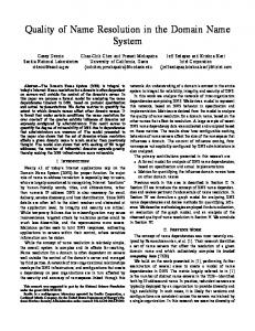
Figure 1: Number of clusters for each cluster size on test+train data (log-log plot shown)
The statistics of the training/test sets and the different sources are shown in Table 1. Despite the fact that both were sampled from the same sources, the ambiguity in the test data (45.93 referents per person, on average) is much higher than in the training data (where it is only 10.76). According to Artiles et al. [3], it shows that “there is a high (and unpredictable) variability, which would require much larger data sets to have reliable population samples.” In order to measure performance as reliably as possible given the SemEval test suite, we conduct our experiments using all names from both the training and the test sets; we will refer to it as all names. While there appears to be high ambiguity due to the large number of person senses given a name, we assumed that the distribution of documents to person senses would follow a power law. Figure 1 shows that the size of the clusters follows a power law with an exponent of approximately 1.31 estimated used linear regression of the log-log plot. This confirms the second assumption of the data and is a novel finding regarding this task/data.
4.2
Performance Measures
Evaluation of the SemEval WePS task is performed using standard clustering measures: purity and inverse purity.
1 , 1 1 α purity + (1 − α) inv.purity
(7)
where α ∈ [0..1] is a parameter to set the ratios between purity and inverse purity. The harmonic mean (α = 0.5) was used for the final ranking of systems at SemEval, and F0.2 was also reported as an additional measure, which gives more importance to the inverse purity aspect (α = 0.2). Artiles et al. [2] argue that the rationale for using F0.2 , from a user’s point of view, is that “it is easier to discard a few incorrect web pages in a cluster which has all the information needed, than having to collect the relevant information across many different clusters.” We decided to also report on F0.8 , a measure which gives more importance to the purity aspect (α = 0.8). Our motivation for also reporting F0.8 is that from a machine point of view, it is more important to ensure that the precision/purity of the clusters are high (so that any subsequent task involving their use, like building a profile, does not contain any unnecessary noise).
4.3
Document Representation
A separate index was built for each person, using the Lemur toolkit.3 We used a standard (English) stopword list but did not apply stemming. A document was represented using the title and snippet text from the search engine’s output, and the body text of the page, extracted from the crawled HTML pages, using the method described below.
4.3.1
Acquiring Plain-Text Content from HTML
Our aim here is to extract the plain-text content from HTML pages and to leave out blocks or segments that contain little or no useful textual information (headers, footers, navigation menus, adverts, etc.). To this end, we exploit the fact that most web pages consist of blocks of text content with relatively little markup, interspersed with navigation links, images with captions, etc. These segments of a page are usually separated by block-level HTML tags. Our extractor first generates a syntax tree from the HTML document. We then traverse this tree while bookkeeping 3
URL: http://www.lemurproject.org
the stretch of uninterrupted non-HTML text we have seen. Each time we encounter a block-level HTML tag we examine the buffer of text we have collected, and if it is longer than a threshold, we output it. The threshold for the minimal length of buffer text was empirically set to 10. In other words, we only consider segments of the page, separated by block-level HTML tags, that contain 10 or more words.
4.4
PLSA Estimation
We used the Lemur toolkit and the PennAspect implementation of PLSA [20] for our experiments, where the parameters for PLSA were set as follows. For each k we perform 10 initializations where the best initialization in terms of log-likelihood is selected. The EM algorithm is run using tempering with up to 100 EM Steps. For tempering, the setting suggested in [11] is used. The models are estimated on 90% of the data and 10% of the data is held out in order to compute the log-likelihood of the decompositions.
5.
EXPERIMENTS AND RESULTS
In this section, we present an experimental evaluation of the two clustering approaches. We address the following specific research questions, leaving the more general ones surrounding the person cluster hypothesis to Section 6: • What factors affect performance? I.e., number of clusters, similarity threshold, similarity metric, etc. • How stable is the performance? • When is the best performance obtained? • What is the best number of clusters to use? Can we determine this automatically? • How do the different clustering approaches compare to each other? We start by exploring the performance and behavior of the SPC and PLSA methods, separately. Then, we compare and contrast the two methods, before providing an analysis over different groups (as opposed to aggregated over all topics).
5.1
Single Pass Clustering
Figures 2 and 3 present the results of the SPC method along a number of dimensions, using the Naive Bayes (SPCNB) and cosine similarity measures (SPC-COS), respectively. Results are aggregated over all names (including both the training and test sets); the best scoring configurations are summarized in Table 3 (columns 2–6). The top left plot shows performance given the maximum number of clusters is fixed (η = 100) as the similarity threshold is varied. The bottom left plots shows the harmonic F-score displayed for various similarity thresholds for η equal to a maximum of 10, 25, 50, and 100 clusters. These two plots across the similarity threshold show that the performance of either SPC is very stable w.r.t. the threshold, but the best performance obtained is with a lower threshold. This implies that the similarity between documents need not be very high (i.e., the evidence to contrary for assignment can be quite low, for assumption 3.). In the top right plots, the similarity threshold is fixed (γ = 0.1) and performance is measured against different maximal cluster size limits. In the bottom right plots, the F-score is explored against the possible cluster sizes, using different
similarity threshold configurations. In these two plots across the maximum number of clusters, we can see that enforcing a limit on the clustering is not appropriate—and actually violates the third assumption. However, this appears to be in contrast with the similarity threshold, which from above, does not need to be very high. Consequently, the best performance was achieved when the maximum number of clusters (η) was set to 100, and this was independent of the similarity measure. And while performance was quite stable given the similarity threshold, γ set to 0.1 was the threshold which delivered the highest F-score.
5.2
PLSA
Experimental condition Manual (truth) Auto (γ = 0.5) Auto (γ = 1.0) Auto (γ = 5.0)
pur. 0.530 0.495 0.517 0.662
invp. 0.647 0.800 0.782 0.647
F0.5 0.547 0.536 0.543 0.561
F0.2 0.591 0.624 0.622 0.583
F0.8 0.530 0.501 0.515 0.584
Table 2: Performance of PLSA. Best scores are in boldface. Results are reported on all names. Table 2 reports on the results we obtained from PLSA under two different experimental conditions. The first is a manual configuration of the number of latent topics which is set to be the actual number of person-senses, based on the ground truth files. This is to determine an upper bound, which could be achieved if the number of latent topics could be identified, and assuming that each latent topic is actually representative of each person-sense. The other more realistic experimental setting uses unsupervised learning to determine the number of latent topics within the set of documents (as explained in subsection 3.2). For this setting, we varied the similarity threshold. Surprisingly, the manual setting did not perform very well at all, and shows that the latent topics are not really that representative of the individual person senses. We suspect this is because the distribution over the latent topics is dominated by only a few (“principal”) components, so to speak; and so the number of resulting clusters is quite low (as we shall see in a following subsection); the automatic methods stop, in theory, when the overriding latent factors have been identified (because using any more would just introduce noise). Consequently, we find that the best performance for PLSA is obtained when the number of clusters is automatically estimated. In contrast to the SPC methods, the number of clusters identified is very low, which results in a high inverse purity, but lower purity (as we anticipated). Interestingly, for PLSA increasing the threshold means that more clusters are created, but at the expense of inverse purity.
5.3
Comparing Methods
Table 3 presents the results achieved by the best performing configuration of the different clustering approaches. The parameters are: λ = 0.5, η = 100, γ = 0.1 for SPC with Naive Bayes similarity (SPC-NB), η = 100, γ = 0.1 for SPC with cosine similarity (SPC-COS), and γ = 1.0 for PLSA.4 4 In case of PLSA, there is no ‘best’ γ, the setting we use is the one that performs well across the board.
0.85
0.9 0.85
0.8
purity inv. purity F0.5
0.75
0.8
purity inv. purity F0.5
0.75 0.7
0.7
0.65
0.65 0.6
0.6 0.55 0.55
0.5
0.5
0
0.5
1
1.5
2 2.5 3 Similarity threshold
3.5
4
4.5
0.45
5
0.63
0
10
20
30
40 50 60 70 Maximum number of clusters
80
90
100
0.62 10 clusters 25 clusters 50 clusters 100 clusters
0.62
0.61 !=0.5 !=1 !=5
0.6 0.61
0.6
F0.5 score
F0.5 score
0.59
0.59
0.58 0.57 0.56
0.58 0.55 0.57
0.54
0
0.5
1
1.5
2 2.5 3 Similarity threshold
3.5
4
4.5
5
0.53
0
10
20
30
40 50 60 70 Maximum number of clusters
80
90
100
Figure 2: Single Pass Clustering using the Naive Bayes similarity measure. (Top Left): varying the similarity threshold, maximum number of clusters is fixed, (Top Right): varying the maximum number of clusters, similarity threshold is fixed, (Bottom Left): varying the similarity threshold, using different cluster size configurations, (Bottom Right): varying the cluster sizes, using different similarity threshold configurations. Results are reported on all names. We can see the contrast between the two methods when we consider the number of clusters each method creates against the actual number of person-senses. Figure 4 plots the number of estimated clusters against the actual number of clusters, extracted from the truth files for each of the clustering methods. Clearly, the SPC method is providing a better estimate of the number of person-senses. This is reflected by the strong correlation between clusters and person senses. The Pearson’s Correlation coefficients for SPC-NB and SPCCOS was r = 0.736 and r = 0.634, respectively —where r = 1 would indicate that the method correctly identifies the true number of person senses. On the other hand, PLSA completely underestimates the number of person senses and the correlation is very weak (r = 0.045). These results clearly demonstrate the difference in the behaviors of the two clustering approaches and that the term based approach (SPC) outperforms the semantic based approach (PLSA). SPC assigns people to the same cluster with high precision, as is reflected by the high purity scores. In contrast with SPC, the PLSA method produces far fewer clusters per person. These clusters may cover multiple referents of a name, as is witnessed by the low purity scores.
On the other hand, inverse purity scores are very high, which means referents are usually not dispersed among clusters.
5.4
Group-Level Analysis
The results we have looked at so far were aggregated over all people. Since the data is not homogenous, it is interesting to see how performance varies on different groups of people. More specifically, we seek to answer: what is the performance of the methods like over (i) different data sources and (ii) different numbers of person senses? Figure 5 shows the performance of SPC and PLSA across the different data sources. All sources display high levels of variability, which seems independent of the size of the source. In case of SPC, the level of variance is more prominent for the US Census than for the other three sets. The median F-scores of US Census and ECDL are in the same range (0.66–0.69), as well as of Wikipedia and ACL06 (0.79– 0.81). However, for PLSA, the deviation is very high for all sources. The median F-scores of Wikipedia and ECDL are in the same range (0.64–0.66), US Census and ACL06 are significantly lower (0.51 and 0.43, respectively). Figure 6 shows the performance of SPC across the dif-
1
0.9 purity inv. purity F0.5
0.9
purity inv. purity F0.5
0.85 0.8
0.8 0.75 0.7
0.7
0.6
0.65 0.6
0.5 0.55 0.4
0.1
0.5
0.2
0.3
0.4
0.5 0.6 Similarity threshold
0.7
0.8
0.9
0.45
1
0.75
0
10
20
30
40 50 60 70 Maximum number of clusters
80
90
100
0.72 10 clusters 25 clusters 50 clusters 100 clusters
0.7
!=0.1 !=0.2 !=0.5
0.7 0.68 0.66
0.65 F0.5 score
F0.5 score
0.64 0.6
0.62 0.6
0.55 0.58 0.56 0.5 0.54 0.45 0.1
0.2
0.3
0.4
0.5 0.6 Similarity threshold
0.7
0.8
0.9
1
0.52
0
10
20
30
40 50 60 70 Maximum number of clusters
80
90
100
Figure 3: Single Pass Clustering using the cosine similarity measure. (Top Left): varying the similarity threshold, maximum number of clusters is fixed, (Top Right): varying the maximum number of clusters, similarity threshold is fixed, (Bottom Left): varying the similarity threshold, using different cluster size configurations, (Bottom Right): varying the cluster sizes, using different similarity threshold configurations. Results are reported on all names. ferent cluster sizes, where the cluster size is the number of senses of a person, based on the ground truth. Interestingly, as the number of senses goes up, so does the F-score achieved by the SPC algorithm. On the other hand, PLSA seems to have an orthogonal effect, the best F-score is achieved when the number of senses is low (≤ 10), and performance is gradually decreasing, as the number of senses increases. This behavior confirms our intuition, that the distribution of latent topics may be dominated by a few principal components, which are easier to associate with prominent person senses, or when there are only a few referents. When only limited examples of the other referents is available (i.e. one or two document, which is often the case according to assumption two), PLSA seems unable to specifically identify such cases. The parameter settings of SPC and PLSA in Figure 5 and 6 correspond to the SPC-COS and PLSA configurations in Table 3.
6.
DISCUSSION AND CONCLUSION
In this paper, we have explored the person clustering hypothesis for the personal name resolution task in a web setting. As we have seen, SPC with a standard bag of words
Method SPC-NB SPC-COS PLSA CU COMSTEM IRST-BP PSNUS ONE-IN-ONE ALL-IN-ONE
pur. 0.884 0.850 0.370 0.720 0.750 0.730 1.000 0.290
invp. 0.688 0.777 0.885 0.880 0.800 0.820 0.470 1.000
F0.5 0.747 0.791 0.442 0.780 0.750 0.750 0.610 0.400
F0.2 0.707 0.780 0.581 0.830 0.770 0.780 0.520 0.580
Table 4: Comparison of results to baselines and top performing systems at the SemEval 2007 WePS task. Results are reported on the test set only.
representation, provides excellent performance on this task. To put this into context, Table 4 reports the results of our best performing methods, along with the top performing systems from SemEval[3] and two naive baselines; ONE-INONE, which assumes that each document is a different referent (i.e., the worst case scenario of assumption 3, if we had no evidence), and ALL-IN-ONE, which assumes that
80
70
50
40
30
20
50 Estimated number of person senses
60
50
40
30
20
0
10
20
30 40 50 60 70 Actual number of person senses (key)
80
90
100
0
40
30
20
10
10
10
0
60
60
Estimated number of person senses
Estimated number of person senses
70
0
10
20
30 40 50 60 70 Actual number of person senses (key)
80
90
100
0
0
10
20
30 40 50 60 70 Actual number of person senses (key)
80
90
100
Figure 4: Estimated versus actual number of person senses. (Left) SPC-NB, (Middle) SPC-COS, (Right) PLSA. The Pearson correlation coefficient r is 0.736, 0.634, and 0.045, respectively. Method SPC-NB SPC-COS PLSA
pur. 0.828 0.808 0.517
All names invp. F0.5 F0.2 0.562 0.623 0.579 0.641 0.681 0.651 0.782 0.543 0.622
Training set F0.8 pur. invp. F0.5 F0.2 0.705 0.793 0.484 0.547 0.501 0.736 0.782 0.557 0.613 0.572 0.515 0.607 0.719 0.605 0.647
Test set F0.8 pur. invp. F0.5 F0.2 0.641 0.884 0.688 0.747 0.707 0.688 0.850 0.777 0.791 0.780 0.596 0.370 0.885 0.442 0.581
F0.8 0.809 0.815 0.382
Table 3: Results achieved by the best performing configurations of the different approaches. Best scores are in boldface. all documents are associated with one referent. While two of these top performing systems use richer features and more sophisticated clustering methods, the performance of SPCCOS is comparable, if not state of the art, and provides a strong baseline for this task. This is truly remarkable, and demonstrates that viewing the task of person name resolution as document clustering is quite effective. Furthermore, we contend that this result, provides strong evidence to suggest that the “person cluster hypothesis” holds to a large extent. While the way in which we used PLSA for this task has not performed as well as we expected, we have identified a number of possible reasons for this failure. We also noted that when there are only few person senses PLSA is more effective than SPC. An interesting line of future work would be to consider how the advantages of both methods could be combined in order to gain greater improvements. Other areas for future research where improvements could be gained include employing a richer feature set which includes named entities, etc., and pre-processing the documents to remove irrelevant content before the disambiguation process.
7.
ACKNOWLEDGMENTS
Balog and De Rijke were supported by the Netherlands Organisation for Scientic Research (NWO) under project numbers 220-80-001, 600.065.120 and 612.000.106. De Rijke was also supported by NWO under project numbers 017.001.190, 264-70-050, 354-20-005, 612-13001, 612.066.302, 612.066.512, 612.069.006, 640.001.501, 640.002.501, and by the E.U. IST programme of the 6th FP for RTD under project MultiMATCH contract IST-033104.
8.
REFERENCES
[1] R. Al-Kamha and D. W. Embley. Grouping search-engine returned citations for person-name queries. In WIDM ’04: Proceedings of the 6th annual ACM international workshop on Web information and data management, pages 96–103, New York, NY, USA, 2004. ACM Press.
[2] J. Artiles, J. Gonzalo, and F. Verdejo. A testbed for people searching strategies in the www. In SIGIR ’05: Proceedings of the 28th annual international ACM SIGIR conference on Research and development in information retrieval, pages 569–570, New York, NY, USA, 2005. ACM Press. [3] J. Artiles, J. Gonzalo, and S. Sekine. The SemEval-2007 WePS Evaluation: Establishing a benchmark for the Web People Search Task. In Proceedings of Semeval 2007, Association for Computational Linguistics, 2007. [4] A. Bagga and B. Baldwin. Entity-based cross-document coreferencing using the vector space model. In Proc. 36th Annual Meeting of the Association for Computational Linguistics (ACL) and 17th Conf. on Computational Linguistics (COLING), pages 79–85, 1998. [5] R. Bekkerman and A. McCallum. Disambiguating web appearances of people in a social network. In Proceedings of the 14th International World Wide Web (WWW) Conference, pages 463–470, 2005. [6] D. Bollegala, Y. Matsuo, and M. Ishizuka. Extracting key phrases to disambiguate personal name queries in web search. In Proceedings of the Workshop on How Can Computational Linguistics Improve Information Retrieval? at ACL’06, pages 17–24, 2006. [7] N. Craswell, A. de Vries, and I. Soboroff. Overview of the TREC-2005 Enterprise Track. The Fourteenth Text REtrieval Conference (TREC 2005) Proceedings, 2006. [8] M. Fleischman and E. Hovy. Multi-document person name resolution. In Proc. 42nd Annual Meeting of the Association for Computational Linguistics (ACL), Reference Resolution Workshop, 2004. [9] C. Gooi and J. Allan. Cross-document coreference on a large scale corpus. In Proc. Human Language Technology/North American chapter of Association for Computational Linguistics annual meeting (HLT/NAACL),, pages 9–16, 2004. [10] D. R. Hill. A vector clustering technique. In Samuelson, editor, Mechanised Information Storage, Retrieval and Dissemination, North-Holland, Amsterdam, 1968. [11] T. Hofmann. Probabilistic latent semantic analysis. In Proc. of Uncertainty in Artificial Intelligence, UAI’99, Stockholm, 1999. URL citeseer.ist.psu.edu/ hofmann99probabilistic.html. [12] N. Jardine and C. J. van Rijsbergen. The use of hierarchic clustering in information retrieval. Information Storage and Retrieval, 7:217–240, 1971.
0.9
0.9
0.8
0.8
0.7
0.7
0.6
0.6 F
0.5
1
F0.5
1
0.5
0.5
0.4
0.4
0.3
0.3
0.2
0.2
0.1
0.1 US_Census
Wikipedia
ECDL
ACL06
US_Census
Wikipedia
ECDL
ACL06
Figure 5: Performance of SPC (Left) and PLSA (Right) across the different data sources
0.9
0.9
0.8
0.8
0.7
0.7
0.6
0.6 F
0.5
1
F0.5
1
0.5
0.5
0.4
0.4
0.3
0.3
0.2
0.2
0.1
0.1 X