QUT Digital Repository: http://eprints.qut.edu.au/
Liang, Huizhi and Xu, Yue and Nayak, Richi (2009) Personalized Recommender Systems Integrating Social Tags and Item Taxonomy. In: 2009 IEEE/WIC/ACM International Conference on Web Intelligence and Intelligent Agent Technology Workshops, September 15-18, 2009, Milano, Italy.
©
Copyright 2009 IEEE
20092009 IEEE/WIC/ACM IEEE/WIC/ACM International International Conference Joint Conference on Web Intelligence on Web Intelligence and Intelligent and Intelligent Agent Technology Agent Technology - Workshops
Personalized Recommender Systems Integrating Social Tags and Item Taxonomy Huizhi Liang, Yue Xu, Yuefeng Li, Richi Nayak, Li-Tung Weng School of Information Technology Queensland University of Technology, Brisbane, Australia
[email protected], {yue.xu, y2.li, r.nayak}@qut.edu.au,
[email protected] Abstract
explicitly and proactively, implying users' interests and preferences information, and being relatively small in data size. Thus, social tagging is becoming an important new implicit rating information source besides users' click stream and browsing history etc. to profile users' interests for making personalized recommendation [2], improving personalized searching [3] and generating user and item clusters [4] etc. However, since there is no any restriction or boundary on selecting words for tagging items, the tags used by users are free-style, lack in standardization and also contain a lot of ambiguity, which causes low information sharing and inaccurate user profiling. Besides, both the items and tags follow the power law distribution, which means only a small number of items or tags are being used by many users while the majority items or tags only used by a small number of users [4]. The free-style vocabulary and the power law distribution of items and tags bring challenges to generate proper neighbourhood for making recommendation through calculating the tag and item overlaps, which causes low recommendation performances. On the other hand, each item itself is associated with a set of controlled vocabulary directly or indirectly, such as item's keywords, taxonomy and ontology etc. Item taxonomy is a set of controlled vocabulary terms or topics designed to describe or classify items, which is available for various domains, for example, the book classification taxonomy of Amazon.com, world knowledge ontology such as Library of Congress Subjects Headings [5]. Because item taxonomy is usually designed and developed by experts, it reflects the common views to the description and classification of items, and provides not only a standard vocabulary but also a hierarchical structure to represent the relationships among concepts or categories, therefore, it can be used to eliminate the inaccuracy caused by users’ free-style vocabulary in social tags as well as improving the low information sharing caused by the long tails [4] of tags and items. In this paper, we propose to integrate user
The social tags in web 2.0 are becoming another important information source to profile users' interests and preferences to make personalized recommendations. To solve the problem of low information sharing caused by the free-style vocabulary of tags and the long tails of the distribution of tags and items, this paper proposes an approach to integrate the social tags given by users and the item taxonomy with standard vocabulary and hierarchical structure provided by experts to make personalized recommendations. The experimental results show that the proposed approach can effectively improve the information sharing and recommendation accuracy.
1. Introduction Recommender System is one effective tool to deal with information overload issue. In practice, one drawback of recommender systems is the insufficiency of user explicit rating [1] information towards items, which causes low recommendation performances. Thus, how to make recommendation based on users’ implicit rating information has become an important research problem. In web 2.0, user's explicit textural information such as tags, blogs, reviews and comments etc. is becoming more and more popular. Instead of using numeric numbers, people use one or more pieces of textural information to express their opinions and interest, collect and organize items, share experiences, and build up social networks etc. These kinds of information provided by users and processed by the “wisdom of crowds” are becoming another important information resource besides the information provided by the websites. Social tags are a kind of typical web 2.0 information, which include one or more keywords provided by users to label and organize items. Social tags have been used in various web application areas, such as del.ici.ous, CiteULike, Amazon.com, and LibraryThing. Tags have distinctive advantages such as being given by users 978-0-7695-3801-3/09 $26.00 © 2009 IEEE DOI 10.1109/WI-IAT.2009.89
540
better recommendations. Although, some researchers have discussed about how to combine item taxonomy with users' implicit ratings to make better recommendation such as Zieglar's work [10] and Weng’s work [11] etc., they didn’t consider tag information, which, makes the proposed approach different from their work.
contributed social tags and expert developed item taxonomy together to make personalized recommendations. Section 2 will briefly review the related work. In Section 3, after giving some definitions, we will firstly describe a novel method to find the semantic representation of each tag based on the taxonomic information of the items in that tag, then the user profile generation, neighbourhood formation, and recommendation generation approaches will be discussed. In Section 4, we will discuss the experimental results and evaluations. The conclusion will be given in Section 5.
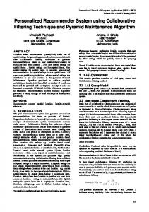
3. Proposed Approach 3.1 Definitions For easy describing the proposed approach, we define some concepts and entities as below. In this paper, topics, concepts, categories and nodes are interchangeably used. x Users: = { 1 , 2 , … , } contains all users in an online community who have used tags to organize items. x Items (or Products, Resources): = { 1 , 2 , … , } contains all items tagged by users in U. We assume that each item p can be described by a set of tags given by users and a set of item taxonomic topics given by experts. x Tags: = { 1 , 2 , … , } contains all tags used by the users in U. x Item Taxonomy: =< , >, = is a set of topics or 0, 1, 2, … , categories given by experts to describe or classify items and = { 1 , 2 , … , } is a set ∈ . of relations between any ∈ and If R=Ф, then W is only a set of topics and no relationships are considered. In this paper, we only use the typical hierarchical relationship. We redefine R = {r}, r is a “sub topic of” relationship, for , ∈ , if , then is a sub topic of . The taxonomy tree has exactly one root topic, which is denoted as ┬ and represents the most general topic. The leaf topics that don’t have direct sub topics represent the most specific topics and are denoted by ┴. x Item taxonomic descriptors: Each item p is associated with a set of item taxonomic ( ) = 1, 2, … , descriptors . A taxonomic descriptor is a sequence of ordered taxonomic topics, denoted by = 0, , , … , , 0, , , … , ∈ , =┴, and … 0 =┬, 0. An item is allowed to be described with multiple descriptors because the item might possess a broad range of concepts. Figure 3.1 shows an example of item taxonomy.
2. Related Work Recommender systems have been an active research area for more than a decade, and many different techniques and systems with distinct strength have been developed. Recommender systems can be broadly classified into three categories: content-based recommender systems, collaborative filtering based recommender systems and hybrid recommender systems. Typically, users' explicit numeric ratings towards items are used to represent users' interests and preferences to find similar users or similar content items to make recommendations. However, because users' explicit rating information is not always available, the recommendation techniques based on user's implicit ratings have drawn more and more attention recently. Besides the web log analysis of users' usage information such as click stream, browse history and purchase record etc., users' textural information such as tags, blogs, reviews in web 2.0 becomes an important implicit rating information source to profile users' interests and preferences to make recommendations [4]. Currently, the researches about tags in recommender systems are mainly focused on how to recommend tags to users such as using the co-occurrence of tags [4] and association rules [6] etc. Not so much work has been done on the item recommendation. Although there are some recent work discusses about content based recommender system integrating tag information [7], hybrid recommendation approach using probabilistic latent semantic analysis (PLSA) approach in folksonomies [8], extending the user-item matrix to user-item-tag matrix to make collaborative filtering item recommendation etc, more advanced approaches of how to exploit tags to improve the performances of item recommendations are needed. In our previous work [9], we proposed a recommendation approach based on the derived user-item, user-tag and tag-item sub matrixes. But the performances still need to be improved. In this paper, we propose an approach to integrate social tags and item taxonomy to make 541
Books
Level 1
C0 C1
C2
Business
Romance
C4 Small Business C8 Online Auctions
C9 Auditing
C3 Computers C6
C5
Networking
C7 Databases
Level 3
C11 Game Programming
C12 Languages
Level 4
Programming
C10 Web Development
Level 2
C13 Java
Figure 3.1 An example of item taxonomy D(p) be the set of item taxonomic descriptors associated with item p, then ( ) = { ( )| ∈ ( ) } is the set of item taxonomy descriptors for tag t. Apparently, D(t) reflects the expert's viewpoint that the taxonomic topics in D(t) can be used to describe the items in P(t), while tag t represents users' point of view that t can be used to describe the items in P(t). Thus, the aim of this section is to generate a set of taxonomic topics from D(t), to represent the semantic meaning of t. Let ( ) be the semantic representation of tag t that is derived from D(t), ( ) can be represented as a set of topics along with a weight for each topic: ( ) = {( , )| ∈ , > 0} (3.1) is the weight of and ∑ = 1. The Where, calculation of the weight of each topic is very important. One common approach is to calculate the frequency of each topic in D(t) and use the frequency as the weight. However, because each descriptor starts from the root, many descriptors share common topics at upper levels. Therefore, the topics at upper levels usually have higher frequency than the topics at lower levels. If we use the frequency of a topic as its weight, those more general topics at upper levels will be treated more important than those more specific topics at lower levels since the topics at higher levels have a higher frequency, which is not always true. That means, we should take the effect of levels into consideration to calculate the weight of topics. In the following subsections, we firstly present a method to estimate the level weight of the taxonomy tree, then a method to calculate the weight of topic . Finally, we discuss how to represent tag t with selected taxonomic topics.
Example 1 (Descriptors) Suppose that 1 is a book which is described by three descriptors 1 , 2 , 3 , where 1 = ( 0 , 3 , 5 , 10 ), 2 = ( 0 , 3 , 7 ), 3 = ( 0 , 3 , 5 , 11 ). From Figure 3.1, we can see that the three taxonomic descriptors are (Books, Computers, Programming, Web Development), (Books, Computers, Database) and (Books, Computers, Programming, Game Programming).
3.2 Semantic Representation of Tags As mentioned in Introduction, user-defined tags are free-style and lack in standardization. As uncontrolled vocabularies, social tags suffer from many difficulties such as ambiguity in the meaning of and differences between terms, a proliferation of synonyms, varying levels of specificity, and lack of guidance on syntax and slight variations of spelling and phrasing [4], which causes inaccuracy and low information sharing and consequently, low recommendation performances. To solve this problem, in this section, we propose an approach to extract the semantic meaning of a tag based on the taxonomic descriptors of the items in that tag. In a tag, a set of items are gathered together according to users’ viewpoint. We believe that there must be some correlation between the user’s tag and the categories of the items in that tag. Otherwise the user may not classify the items into that tag. Thus, by combining the tags and the taxonomy of the items in the tags, we can derive a set of item taxonomic categories or topics along with the structural relationship among them to represent the semantic meaning of each tag. Since the taxonomic topics belong to a set of controlled vocabulary, the information sharing among users can be more precisely captured. For each tag t ∈ T, it has a set of items that are collected and classified to this tag by one or more users of U, which is denoted as P(t), P(t)⊆P, Let
3.2.1 Taxonomy Level Weighting As discussed above, topics at higher levels have higher frequencies because of their positions in the descriptors (i.e, the levels in the taxonomy tree). If 542
topic at level j+1 must have a link to a non-leaf topic at level j. That means the topics at level j+1 occur if and only if the non-leaf topics at j occur. Therefore, the probability of topics at level j+1 occurring in descriptors given topics at level j can be measured by the ratio of non-leaf topics at level j. The equation to calculate (j + 1| j) is given below: | ( )| − | ( )| ( + 1) = ∙ () | ( )| ( )| |L(k)|−| j = ∏k=1 j=1… M-1 (3.3) |L(k)|
we use the frequency to measure the importance of topics to the tag which contains the topics, the effect coming from the level of the topics should be considered. Since the frequency of topics decreases from the top level down to the bottom level, the weight of levels should increase from the top level to the bottom level. Moreover, because the topics at the same level usually have similar frequency magnitude since they are at the same position in descriptors and have the same number of super categories, and usually the probability of the topics at a level occurring in descriptors decreases with the increase of the depth of the level, we propose to estimate the level weight using the reverse of the probability of the topics at that level. In this subsection, we firstly propose a method to determine the number of levels in the taxonomy tree, then present a method to estimate the weight of each taxonomic level based on the reverse of the probability of the occurrence of the topics at that level, and the level weights will be used to determine the portion of the topic frequency contributed to the weight of the topic in Equation 3.1. If W is a complete tree, then all the leaf nodes are at the same level and any descriptors will include all the levels in W. In this case, the number of levels is the actual height of the tree and the weight of each level is the same. However, in real world, the item taxonomy tree is usually incomplete. It means that leaf nodes may be at different levels. In order to include most of the leaf nodes in the bottom level, we choose the depth of most leaf nodes as the height of the taxonomy tree denoted as M. The nodes with depth less than M are kept at their depth level. The nodes with depth larger than or equal to M are included into level M. Thus, all nodes are allocated into M levels. Let L(j) be the set of nodes (i.e., topics) at level j, ≤ − 1, ℎ( ) be the depth of , then ( ) = { | ℎ( ) = ( )={ | ℎ( ) ≥ }, }. , For example, in Figure 3.1, there are 4 levels. The weight of each level is obtained through calculating the reverse of the probability of topics at each level. Let (j) be the probability of topics at level j, (j + 1| j)be the probability of topics at level j+1 giving j, according to Bayes rule, (j + 1) can be calculated with the Equation 3.2 below. (j+1| j)∙ ( ) (j + 1) = j=1…M-1 (3.2)
) is the set of leaf nodes with depth Where, ( of j. Because the root topic (i.e., topic ‘Book’ in Figure 3.1) is the most general topic and it appears in every descriptor, we set the weight of root topic to 0 and the weight of root level to 0. Let ( ) denote the weights of topic and level j and in the taxonomy structure respectively, then 0 = (1) = 0 respectively. Moreover, since all 0 and the meaningful descriptors should at least have two levels which are the root level 1 and level 2, the probability of level 2 occurring in D(t) is 1, which is denoted as (2) = 1. Because the sub taxonomy tree formed by the descriptors of D(t) may only cover less than M levels, to normalize the total level weight, we ( ( ) ( ) = 1. M(D(t)) is the number suppose ∑ =2 of levels covered by the sub taxonomy tree formed from the descriptors in D(t). As we mentioned above, we propose to estimate the level weight using the reverse of the probability of that level. Therefore, the weight for levels from j=2 to M(D(t)) would be 1, 1 1 1 , (4),…, ( . In order to normalize the (3) weights to make ∑ ()=
( ( ))) ( ( )) =2 1
∙
(j)
( ) = 1, we set (3.4)
Thus, after solving the Equation 3.5 below, we can get the value of the factor x and thus the weights of all the levels in D(t) can be obtained by Equation 3.4. 1 ∑M(D(t)) ∙ (j)=1 (3.5) j=2 Leaf nodes are the most specific topics along the path from the root to a leaf node and tend to have low occurrence than non-leaf nodes no matter which level they are. Thus, it’s unfair to compare the occurrences with other non-leaf nodes in the same level. Therefore, we move those leaf nodes with depth 0 (3.6) where ( ) is the level weight of , ∈ ′ ( ), ( ) = ( ), j=1..M. And ( ) is the frequency of in its level in D(t), ( ) = ( )/ ∑ ∈ ′( ) ( ), ( ) is the count of occurrence of in D(t). We can see that the weight of each topic is computed based on the distribution of topics at the same level. The leaf topics will get higher weight than their upper levels. Thus, the free-style social tags that given by users can be converted to a set of standard and relatively small sized item taxonomic topics given by experts, which can eliminate the differences of user tag vocabularies, incorrect syntax and spelling and semantic ambiguity etc. Example 3 (Tag Representation) Assume the user 1 in Example 2 has another tag 2 , 2 = { 2 , 3 }. The descriptors of the books 2 and 3 are: 2 = { 4 }, 3 = { 1 , 4 } . As defined in Example 1 and Example 2, 1 = { 1 , 3 }, 1 = { 1 , 2 , 3 }, 3 = { 1 , 4 }. 1 = ( 0 , 3 , 5 , 10 ), 2 = ( 0 , 3 , 7 ), 3 = ( 0 , 3 , 5 , 11 ), 4 = ( 0 , 1 , 4 , 8 ). The tag 1 and 2 can be represented respectively as follows: 1 ( 1 ) = {( 0 , 0), ( 1 , (0.22 ∙ )), ( 3 , (0.22 ∙ 5 1 5
5
3
)), ( 4 , (0.33 ∙ )), ( 5 , (0.33 ∙ )), ( 7 , (0.45 ∙ )), (
4 2
4 1
5
5
10 , (0.45 ∙ )), ( 8 , (0.45 ∙ )), ( 2
11 , (0.45
), (
10 , (0.45
3
∙ ))} 3
User profile is used to describe user's interests and preferences information. Usually, a user-item rating matrix is used in collaborative filtering based recommender systems to profile a user's item interests and preferences. With the tag information, a user can be preliminarily described with a matrix (user, (tag, item)), where (tag, item) is a sub matrix of each user. The long tails of items and tags cause the sizes of user-item, user-tag, tag-item matrixes are big but the overlaps of items, tags or tag-item sub relationships between users are very low, which makes it difficult to find similar users. One effective way to improve information sharing is to find users’ common information topic interests besides the common item ratings or item preferences. Currently, some approaches have been proposed to generate user's taxonomic topics through converting the user-item rating vector into user-taxonomic topic vector [10]. However, these approaches didn't consider the social tag information. We believe that the user tagging information well reflects user’s interests and should be used to profile users, especially users’ topic interests. We profile user with item preferences and topic preferences, which is denoted by ={ ′ , ′′ }. ′ is ’s item preferences and can be represented by a |P|entry vector, denoted as ′ = ′ ,1 , ′ ,2 , ′ , , . . . , ′ ,| | , ′ , = 1 if has item doesn’t have item . ′′ is the while ′ , =0 if topic preferences of . How to generate ′′ is the major focus of this sub section. Since user’s tags reflect user’s topic interests, we profile each user with a set of tags and their has used. Let = interest scores that , , . . . , , , , … , be the tag set of ,1 , , ,1 , , , ( , ) be the score to measure how much is interested in , , then the score vector ( , ) will represent ’s ( ,1 ), , ,…, interest distribution, which are used to profile . In order to facilitate the similarity measure of any two users, user-wise normalization is applied. We suppose each has the same total interest score S and ∑ =1 = (3.7) , Where S is the normalization factor, which can be any positive number, in this paper we set S=|C|. A common sense is that, if a user is more interested in a topic, usually the user may collect more items
3.2.2 Tag Representation
1
1
3 1
3.3 User Profile Generation
Pr (2) = 1; Pr (3) = 1 ∙ (3 − 1)⁄3 = 2⁄3 ; Pr (4) = 1 ∙ 2⁄3 ∙ (4 − 1)⁄4 = 1⁄2 ; ∙ 1 + ∙ 3⁄2 + ∙ 2 = 1; = 0.22; The weights of these four levels are (1) = 0, (2) = 0.22, (3) = 0.33, (4) = 0.45. Also, from the given topic nodes in Figure 3.1, we can get the following topic level set: ′ (1) = { 0 }, ′(2) = { 1 , 3 , … }, ′(3) = 4 , 5 , 6 , 12, … , ′(4) = 2, 7, 8 , 9 , 10, 11, 13, … .
4
2
)) , ( 4 , (0.33 ∙ ), ( 5 , (0.33 ∙ ), ( 8 , (0.45 ∙
1
∙ ))} 5
( 2 ) = {( 0 , 0), ( 1 , (0.22 ∙ )), ( 3 , (0.22 ∙ 3
544
about that topic. That means, the number of items in a tag is an important indicator about how much the user is interested in the tag. Let ( , ) denote the number of items in tag , we use , used by user the proportion of ( , ) to the total number of items in all tags of to measure the user's interest to tag can be calculated with Equation , . Thus, , 3.8. =
,
∙∑
(
, )
=1 (
, )
with standard neighbourhood for a target user “best-K-neighbours” technique involves computing the distances between and all other users and selecting the top K neighbours with shortest distances to . Based on user profiles, the similarity of users can be calculated through various proximity measures. Pearson correlation and cosine similarity are widely used to calculate the similarity based on numeric values. For the binary rating data, a simple but effective way to compute user similarity is to calculate the overlap of two users’ item sets. The higher the overlap, the more similar the two users are. Based on the user profiles discussed in Section 3.3, for any two users and with profile and , the similarity measure includes two parts: the similarity of item preferences denoted as , and the similarity of topic preferences denoted as , . The similarity of item preferences is measured by the overlap of users’ item sets. The maximum item number that a user has is used to normalize the overlap value to facilitate the comparison of different users, which is defined as below:
(3.8)
Thus, we can obtain the user-tag vector with Equation 3.8. As discussed in Section 3.2, a tag can be represented with a set of taxonomic topics derived from the items that the tag has. We can calculate the score of each taxonomic topic , in each tag , for user as below: = ∙ ∙ , , , , , = 1. . , = 1. . (3.9) Therefore, the topic preferences represented with are converted to topic tags of each user preferences represented with taxonomic topics, which can be modelled by a |C|-entry vector, denoted as ′′ = ′′ ,1 , ′′ ,2 , ′′ , , … , ′′ ,| | , |C| is the total number of topics of C, |C|=q. For each ′′ , in ′′ , the score of ′′ , represents the degree of 's interests and preferences towards taxonomic topic , which is denoted as ( ). ( ) = ∑ =1 (3.10) , Each user can be profiled with the combination of user-item vector ′ and user-topic vector ′′ , which is denoted as: ={ ′ , ′′ }= ′
,1 ,
′
,2 ,
′
,
,...,
′
,| |
,
′′
,1 ,
′′
,2 ,
′′
,
,...,
′′
,
| ′,
′
′ , = , =1, =1..| | }| ′ max 1≤k ≤|U | (|{ , | ′ , =1, =1..| |}|)
(3.12)
The Pearson correlation is used to calculate the similarity of topic preferences, which is defined as below: ,
=
∑ =1( ′′, − ′′ )∙( ′′, − ′′ ) ∑ =1 ( ′′, − ′′ )2 ∙∑ =1 ( ′′, − ′′ )2 )
(3.13)
Therefore, the similarity of and can be measured with Equation 3.14. , = ∙ , + (1 − ) ∙ , ∈ [0,1] (3.14) Using the similarity measure approach, we can generate the neighbourhood of target user , which includes K nearest neighbour users who have similar implicit item ratings and taxonomic topic preferences with ,. The neighbourhood of , is denoted as: Ň( ) = { | , , , where maxK {} is to get the top K values.
,| |
′′ , ∈ [0, ] , ∈ {0,1}, Similarly, an item can be profiled by the taxonomic topic vector, denoted as = , , , . . . , . For each in , the score ,1 ,2 , ,| | , of , represents the degree of item belongs to taxonomic topic , which is denoted as ′( ). For each item , ∑ =1 ′ , = . ′ = ∙ ∙ , = 1. . (3.11) is the frequency of in D( ). Where,
,
=
′
3.5 Recommendation Generation
Example 4 (Topic Preference) We suppose S=100. For the defined user 1 in Example 2 and Example 3, ( 1 )=50, ( 2 )=50. After applying Equation 3.9 and Equation 3.10, we can get the score of topics. ( 1 ) =9.53, ( 4 )=15.12, ( 8) For example, =19.5.
For each target user , a set of candidate items will 's neighbourhood formed be generated from through the measure of the similarity of users, which is denoted as Č( ), , Ň( ), ∉ ( )}. Č( ) = { | Where is the item set of user as defined in Section 3.2. For each candidate item Č( ), let the users in Ň( ) who have the item denoted as may Ň( , ), the prediction score of how much
3.4 Neighbourhood Formation Neighbourhood formation is to generate a set of like-minded peers for a target user. Forming a 545
be interested in can be measured from the aspects of how similar those users who have the item are and how similar the item's taxonomic topics with 's taxonomic topic interest are. Thus, the prediction score denoted as ( , ) can be calculated with Equation 3.15. ( ,
)=
(
,
)∙∑ |Ň(
Ň(
,
,
)|
)
,
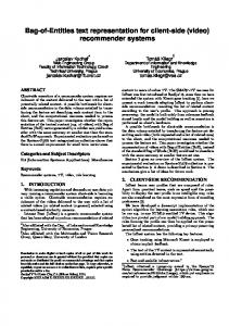
standard collaborative filtering (CF) approach [1] that uses the implicit item ratings or item preferences only. To evaluate the performances of the approaches in different situations, we conducted the comparison experiments with two datasets Dataset 1 and Dataset 2. Dataset 1 is the whole dataset covering all users' information, which is to evaluate the effectiveness in normal situation. The average number of books that a user has is 16.73. Dataset 2 is to evaluate the effectiveness when the dataset is very sparse. We selected 1000 users that each user has no more than 20 books. It includes 1000 users, 4893 books and 5228 tags. The average number of books that a user has is 6.84. The precision and recall results of Dataset 1 are shown in Figure 4.1 and Figure 4.2 respectively, while the precision and recall results of Dataset 2 are shown in Figure 4.3 and Figure 4.4 respectively.
(3.15)
The top N items with larger prediction scores will be recommended to .
4. Experiments and Discussions We conducted the experiments using the dataset obtained from Amazon.com. The items of the dataset are books. In pre-processing, we removed the books that are only used by one user or whose taxonomy descriptors are not available. The final dataset comprises 5177 users, 37120 tags, 31724 books and 242496 records. The book descriptors are also obtained from Amazon.com. The taxonomy formed by these descriptors is tree-structured and contains 9919 unique topics. The precision and recall are used to evaluate the recommendation performance. The whole dataset is split into a test dataset and a training dataset and the split percentage is 50% each. Because our purpose is to recommend books to users, the test dataset only uses users' books information while the training dataset contains users' books and correspondent tags information. The top N items will be recommended to the user. If any item in the recommendation list is in the target user's testing set, then the item is counted as a hit. To evaluate the effectiveness of the proposed approach, we compared the precision and recall of the recommended top N items produced by the following approaches: x Item-Tag-Taxonomic approach, which is the proposed approach that combines implicit item rating and topic preferences generated through integrating tags and item taxonomy. x Tag-Taxonomic approach, which is the proposed approach that only uses topic preferences generated from tags and item taxonomy. x Taxonomic approach, which is proposed by Zieglar's [10] that uses topic preferences generated from item taxonomy only. x Item-tag approach, which is our previous work that uses three derived matrixes user-item, user-tag and tag-item sub matrixes to make recommendation [9]. x Standard CF approach, which is the
Figure 4.1 Precision evaluation of Dataset 1.
Figure 4.2 Recall evaluation of Dataset 1.
Figure 4.3 Precision evaluation of Dataset 2.
Figure 4.4 Recall evaluation of Dataset 2. 546
From the comparison of the proposed TagTaxonomic approach that uses both social tags and item taxonomy and Taxonomic approach proposed by Zieglar [10] that only uses item taxonomy, we can see that the proposed approach outperforms the latter one, which means that the social tags are helpful to mine user’s actual information topic interests and preferences. More importantly, the experimental results show that the proposed approach of integrating social tags and item taxonomy to eliminate the inaccuracy caused by the free-style vocabulary of social tags and to improve the low information sharing caused by the long tails of items and tags for the purpose of improving recommendation accuracy is effective, especially in sparse situation. Besides, we can see that the proposed Item-TagTaxonomic approach that combines item preferences and topic preferences performs better than all the other approaches in both relatively dense and sparse situations. From Figure 4.1 and Figure 4.2, we can see that item preferences intend to play more important part when more books on average each user has. The results in Figure 4.3 and Figure 4.4 show that in very sparse situation, it becomes difficult to find similar users based on users' item preferences or overlaps of items. In this case, the topic preferences intend to play a major role to make recommendations.
This research made an important contribution to better understanding the semantic meaning of social tags and the improvement to the recommendation accuracy of traditional recommender systems (i.e., in e-commerce websites) through incorporating social tags in web 2.0.
References [1] U. Shardanand and P. Maes, “Social Information Filtering: Algorithms for Automating ‘Word of Mouth’”, Proceedings of the SIGCHI conference on Human factors in computing systems, ACM, New York, USA, 1995, pp. 210 -217. [2] K.H.L. Tso-Sutter, L.B. Marinho and L.SchmidtThieme, “Tag-aware Recommender Systems by Fusion of Collaborative Filtering Algorithms”, Proceedings of the 2008 ACM symposium on Applied computing, ACM, New York, USA, 2008, pp.1995-1999. [3] S. Bao, X.Wu, B. Fei,G.Xue,Z.Su,Y.Yu, “Optimizing Web Search Using Social Annotations”, Proceedings of the 16th international conference on World Wide Web, ACM, New York, USA, 2007, pp. 501-510. [4] X. Li, L. Guo, and Y. E. Zhao, “Tag-based social interest discovery”, Proceeding of the 17th international conference on World Wide Web, ACM, New York, USA, 2008, pp. 675-684. [5] The Library of Congress, http://www.loc.gov/. [6] P. Heymann, D. Ramage, and H. Garcia-Molina, “Social tag prediction”, Proceedings of the 31st annual international ACM SIGIR conference on Research and development in information retrieval, ACM, New York, USA, 2008, pp. 531–538. [7] M. de Gemmis, P. Lops, G. Semeraro, and P. Basile, “Integrating tags in a semantic content-based recommender”, Proceedings of the 2008 ACM conference on Recommender systems, ACM, New York, USA, 2008, pp.163-170 . [8] R. Wetzker , W. Umbrath, and A. Said, “A hybrid approach to item recommendation in folksonomies”, Proceedings of the WSDM '09 Workshop on Exploiting Semantic Annotations in Information Retrieval, ACM, New York, USA, 2009, pp. 25-29. [9] H. Liang, Y. Xu, Y. Li, and R. Nayak, “Collaborative Filtering Recommender Systems Using Tag Information”, Proceedings of The 2008 IEEE/WIC/ACM International Conference on Web Intelligence (WI-08) Workshops, 2008, pp. 59-62. [10] C.N. Ziegler, G. Lausen, & L.Schmidt-Thieme, “Taxonomy-driven Computation of Product Recommendations”, Proceedings of the thirteenth ACM international conference on Information and knowledge management, ACM, New York, USA, 2004, pp. 406-415. [11] L.-T. Weng, Y. Xu, Y. Li, and R. Nayak,” Web Information Recommendation Making based on Item Taxonomy”, Proceedings of the 10th International Conference on Enterprise Information Systems, 2008, pp. 20-28.
5. Conclusion In this paper, we propose an approach of combining social tags and item taxonomy to make personalized recommendation. Firstly, we propose an approach to extract tags’ semantic meaning and represent them with taxonomy topics to eliminate the inaccuracy caused by the free-style vocabulary of tags. Then, we propose an approach to generate users’ topic preferences based on users’ interest distribution of their tags. The information sharing among users was improved after converting the user-tag vector into much smaller sized and standard user-taxonomic topics vector. Also, we propose to measure user similarity based on both users’ item preferences and topic preferences generated through the integrating of user contributed tags and expert designed item taxonomy. Finally, a hybrid recommendation generation approach is proposed to recommend the target user those items that not only preferred by the target user’s neighbour users but also similar to the target user’s preferred topics. The experimental results show that the proposed approach outperforms the standard collaborative filtering approach and Zieglar’s approach as well.
547