Noname manuscript No. (will be inserted by the editor)
Perspective Envelopes for Bilinear Functions Hassan Hijazi
Received: date / Accepted: date
Abstract We characterize the convex hull of the set ( S Ă R3 “ px, y, zq P rxl , xu s ˆ ry l , y u s ˆ R | x ď y, z “ xy . The new characterization, based on perspective functions, dominates the standard McCormick convexification approach. In practice, this result is useful in the presence of linear constraints linking variables x and y, but can also be of great value in global optimization frameworks, suggesting a branching strategy based on dominance, i.e., x ď y _ x ě y. The new relaxation yields tight lower bounds, and has the potential to improve the pruning process in spatial branch and bound schemes and consequently reduce the search space effort. Keywords Bilinear Programming ¨ Convex Relaxation ¨ Perspective Function ¨ McCormick Envelopes ¨ Global Optimization
1 Introduction Bilinear expressions are the most common nonconvex components in mathematical formulations modeling problems arising in chemical engineering [20, 19, 26, 8, 38, 12, 37, 10], pooling and blending [13, 5], supply chain and transportation science [16, 35, 34, 36], and energy systems [22, 15, 23, 11], to name NICTA is funded by the Australian Government through the Department of Communications and the Australian Research Council through the ICT Centre of Excellence Program. H. Hijazi NICTA - ORG The Australian National University Canberra ACT 2601 Australia Tel.: +61-2-62676315 Fax: +61-2-62676230 E-mail:
[email protected]
2
Hassan Hijazi
a few. Many convexification approaches [27, 40, 31, 43] are based on the McCormick envelopes [32, 2], these include bound contraction [9], and piecewise McCormick envelopes [10]. Global optimization solvers [6, 1, 39, 33] also heavily rely on these envelopes. Given ( the set S0 “ tpx, y, zq P pB ˆ Rq | z “ xyu , where B “ rxl , xu s ˆ ry l , y u s , Al-Khayyal and Falk [2] were able to define its convex hull in the space of original variables,
$ ’ ’ ’ ’ &
ˇ ˇ ˇ ˇ ˇ ` l u ˘ conv pS0 q “ px, y, zq P rx , x s ˆ ry l , y u s ˆ R ˇˇ ’ ˇ ’ ’ ˇ ’ % ˇ
, / / / u u u u/ z ěx y`y x´x y . z ě xl y ` y l x ´ xl y l
z ď xl y ` y u x ´ xl y u / / / / z ď xu y ` y l x ´ xu y l
This set of constraints, known as the McCormick envelopes, defines the convex and the concave envelopes of the bilinear function f px, yq “ xy on the rectangular domain rxl , xu s ˆ ry l , y u s. The quality of this polyhedral relaxation highly depends on the initial bounds on variables x and y. State-of-the-art global optimization solvers implement bound contraction techniques in order to improve this bounding procedure. Once bound propagation is completed, domain partitioning becomes necessary. Spatial branch and bound schemes [3, 42] are among the most effective partitioning methods in global optimization. By splitting the domain of a given variable, the solver is able to divide the original domain into two smaller regions, further tightening the convex relaxations of each partition. In general, the variables involved in bilinear expressions are also linked through other constraints in the problem formulation. It is thus possible to tighten the convex relaxation of the feasible region by combining the bilinear term with other constraints. Related Work. In [41], the convex hull of the bilinear function over Dpolytopes is derived in the space of original variables. Thereafter, Linderoth [28] produces analytical characterizations on triangular domains. Concurrently, Benson [7] derives the convex hull on parallelograms and trapezoids. More recently, Anstreicher and Burer [4] study higher dimension characterizations. Locatelli and Schoen [30] propose a different approach for computing convex envelopes, based on solving convex programs, Locatelli [29] then uses this result to derive closed-form solutions for specific domains. In this work, we consider the bilinear term xy in conjunction with a dominance constraint linking variables x and y, i.e., x ď y, and leading to polyhedral domains subsuming right triangles, right trapezoids, and rectangles. To the best of our knowledge, there are no analytical characterizations of this convex hull in the space of original variables. The proof, based on perspective functions, offers a new angle on deriving such convex hulls, and can be easily extended to handle arbitrary linear constraints. The main result is presented int the next section.
Perspective Envelopes for Bilinear Functions
3
2 The New Convex Envelope 2.1 Background on perspective functions Perspective formulations have been successfully used to model disjunctive constraints in Mixed-Integer Nonlinear Programming (MINLP) [14, 21, 17], dominating standard big-M formulations. Given a convex function f : Rn Ñ R and a real number u ą 0, the function, fu pxq “ uf px{uq is convex, and represents a dilated version of f [24]. The perspective of f , denoted f˜ : pRn ˆ Rq Ñ pR Y t`8uq, is defined as the operator considering all dilations of f , i.e., # f˜px, uq “
uf px{uq if u ą 0 ` 8 otherwise.
(1)
Figure 1 illustrates the dilation property of the perspective operator on the square function.
Fig. 1 Several dilations of the square function using the perspective operator.
2.2 Notations x denotes a vector variable in Rn , x a variable in R, and x a constant in R. Given a convex domain D Ď Rn , the epigraph of a continuous function f over D, denoted epiD f , is defined as, epiD f “ tpx, zq P D ˆ R | f pxq ď zu .
4
Hassan Hijazi
The convex envelope of f over D, denoted c~ onvD pf q, represents the convex hull of its epigraph, c~ onvD pf q “ conv ptpx, zq P D ˆ R | f pxq ď zuq . The hypograph of f over D, denoted hypoD f , is defined as, hypoD f “ tpx, zq P D ˆ R | f pxq ě zu . The concave envelope of f over D, denoted cz onvD pf q, represents the convex hull of its hypograph, cz onvD pf q “ conv ptpx, zq P D ˆ R | f pxq ě zuq . The projection of a set S on the vector space v is denoted projv S, and its closure is written clpSq.
2.3 The Convex Envelope We first start by stating the following result from [21]. ( ( Lemma 1 [21] Let D0 Ă Rn “ x P rxl0 , xu0 s , and D1 Ă Rn “ x P rxl1 , xu1 s Γ0 “ tpx, uq P D0 ˆ r0, 1s | u “ 0u, and Γ1 “ tpx, uq P D1 ˆ r0, 1s | f pxq ď 0, u “ 1 u , then convpΓ0 Y Γ1 q “ projpx,uq cl pΓ c q , ˇ $ ˇ uf py{uq ď 0 ’ ˇ ’ & ˇ where Γ c “ px, y, uq P R2n ˆ r0, 1s ˇˇ x ´ p1 ´ uqxu0 ď y ď x ´ p1 ´ uqxl0 ’ ˇ ’ % ˇ uxl1 ď y ď uxu1 , 0 ă u ď 1
, / / . / / -
Given a point x˚ P Rn , and a convex set, based on Lemma 1, we characterize the convex hull of their union. ( Corollary 1 Let D Ă Rn “ x P rxl , xu s , Γ0 “ tpx, uq P Rn ˆ r0, 1s | x “ x˚ , u “ 0u , and Γ1 “ tpx, uq P D ˆ r0, 1s | f pxq ď 0, u “ 1 u , then convpΓ0 Y Γ1 q “ cl pΓ c q , ˇ $ ˇ uf ppx ´ p1 ´ uqx˚ q {uq ď 0 ’ ˇ ’ & ˇ where Γ c “ px, uq P Rn ˆ r0, 1s ˇˇ upxl ´ x˚ q ` x˚ ď x ď upxu ´ x˚ q ` x˚ ’ ’ ˇ % ˇ 0ăuď1
, / / . / / -
Proof Set xu0 “ xl0 “ x˚ in Lemma 1. \ [ We now apply this result for the function f : R2 Ñ R, f px, zq “ x2 ´ z.
Perspective Envelopes for Bilinear Functions
5
( Lemma 2 Let D Ă R2 “ px, zq P rxl , xu s ˆ rz l , z u s , Γ0 “ tpx, z, uq P D ˆ r0, 1s |ˇ x “ x˚ , z “ z ˚(, u “ 0u , and Γ1 “ px, z, uq P D ˆ r0, 1s ˇ z ě x2 , u “ 1 , then convpΓ0 Y Γ1 q “ Γ p , where $ ˇ ˇ px ´ p1 ´ uqx˚ q2 ď u pz ´ p1 ´ uqz ˚ q ’ ’ ˇ & ˇ p 2 Γ “ px, z, uq P R ˆ r0, 1s ˇˇ upxl ´ x˚ q ` x˚ ď x ď upxu ´ x˚ q ` x˚ ’ ˇ ’ % ˇ upz l ´ z ˚ q ` z ˚ ď z ď upz u ´ z ˚ q ` z ˚
, / / . / / -
Proof By replacing f pxq with f px, zq “ x2 ´ z in Corollary 1, we have that convpΓ0 Y Γ1 q “ cl pΓ c q , where $ ’ ’ ’ ’ ’ ’ ’ &
ˇ ˇ ˇ ˇ ˇ ˇ ˇ c Γ “ px, z, uq P R ˆ r0, 1s ˇ ˇ ’ ’ ˇ ’ ’ ˇ ’ ’ ˇ ’ % ˇ
ˆ´ u
x´p1´uqx˚ u
¯2 ´
z´p1´uqz ˚ u
˙ ď0
upxl ´ x˚ q ` x˚ ď x ď upxu ´ x˚ q ` x˚
/ / / upz l ´ z ˚ q ` z ˚ ď z ď upz u ´ z ˚ q ` z ˚ / / / / 0ăuď1 , 2 px ´ p1 ´ uqx˚ q ď u pz ´ p1 ´ uqz ˚ q / / / / l ˚ ˚ u ˚ ˚ / upx ´ x q ` x ď x ď upx ´ x q ` x .
ˇ ˇ ˇ ˇ ˇ ˇ “ px, z, uq P R ˆ r0, 1s ˇ ˇ upz l ´ z ˚ q ` z ˚ ď z ď upz u ´ z ˚ q ` z ˚ ’ ’ ˇ ’ ’ ˇ ’ % ˇ 0ăuď1 $ ’ ’ ’ ’ ’ &
, / / / / / / / .
/ / / / / -
Finally, observe that cl pΓ c q “ Γ c Y Γ0 “ Γ p . \ [ This leads to the main lemma, Lemma f px, yq “ xy on the domain ˇ , $ 3 Consider the bilinear function ˇ xďy / ’ ˇ / ’ / ’ ˇ u / ’ u u l / ’ x ´x ˇ x ´y & u. x ď y ` x l u l u ˇ c D “ px, yq P rx , x s ˆ ry , y s ˇ xl ´ y u xl ´ y u ˇ / ’ / ’ l u ˇ / ’ ’ y ´y y l ´ xl / ’ ˇ l / % x ě y ` y ˇ l x ´ yu xl ´ y u s.t. xl ă y u , then c~ onvDc pf q “ P c , where " P “ px, y, zq P Dc ˆ R c
and δ “ pxl ´ y u q.
ˇ ˆ ˙2 ˆ ˙ˆ ˙ ˇ x´y l ux ´ y ˇ x ´ xl x ´ y ď 1´ z´x y ˇ δ δ δ
* ,
6
Hassan Hijazi
Proof Let u “ 1 ´
px´yq δ ,
we have that
u “ 0 ô x ´ y “ xl ´ y u ô x “ xl and y “ y u u“1ôx“y Since x ď y on Dc , we can assume w.l.o.g. that xl ď y l and xu ď y u , if y l ă xl , we can safely update the lower bound on y, i.e., set y l “ xl . A similar ( reasoning applies for the upper bound. Consequently, z l “ min xl y u , xl y l ( and z u “ max xu y u , xl y u . ˇ ( Let Γ0c “ px, z, uq P rxl , xu s ˆ rz l , z u s ˆ r0, 1s ˇ x “ xl , z “ xl y u , u “ 0 , ˇ ( and Γ1c “ px, z, uq P ry l , xu s ˆ rz l , z u s ˆ r0, 1s ˇ x2 ď z, u “ 1 . Observe that the lower bound on x is y l for u “ 1 (x “ y and xl ď y l ). Based on Lemma 2, we have that conv pΓ0c Y Γ1c q “ Γ p , where $ ’ ’ & p Γ “ px, y, zq P R3 ’ ’ %
, ˇ ` ˇ x ´ p1 ´ uqxl ˘2 ď u `z ´ p1 ´ uqxl y u ˘ / ˇ / . ˇ ˇ upy l ´ xl q ` xl ď x ď upxu ´ xl q ` xl ˇ / ˇ / ˇ upz l ´ xl y u q ` xl y u ď z ď upz u ´ xl y u q ` xl y u -
Using the variable substitution u “ 1 ´ px ´ yq{δ, we have that `
x ´ p1 ´ uqxl
˘2
` ˘ ď u z ´ p1 ´ uqxl y u õ
ˆ
lx
x´x
´y δ
˙2
ˆ ď
x´y 1´ δ
˙ˆ ˙ l ux ´ y z´x y . δ
Similarly, xu ´ y u xď xl ´ y u yl ´ yu upy l ´ xl q ` xl ď x ô l xě x ´ yu
upxu ´ xl q ` xl ě x ô
xu ´ xl y ` xu , xl ´ y u y l ´ xl y ` yl , xl ´ y u
upz l ´ xl y u q ` xl y u ď z ô pz l ´ xl y u qpy ´ xq ě δpz ´ z l q, upz u ´ xl y u q ` xl y u ě z ô pz u ´ xl y u qpy ´ xq ď δpz ´ z u q. It is easy to check that the constraint upz l ´ xl y u q ` xl y u ď z (respectively x ď y) is strictly redundant in Γ0c (resp. Γ1c ), and weakly redundant in Γ1c
Perspective Envelopes for Bilinear Functions
7
(resp. Γ0c ), thus it is not facet defining in conv pΓ0c Y Γ1c q. Therefore, ˇ ˆ ˙2 ˆ ˙ˆ ˙, ˇ x´y l ux ´ y / ˇ x ´ xl x ´ y . ď 1´ z´x y ˇ δ δ δ Γp “ px, y, zq P Dc ˆ R ˇ . ˇ u ’ / % ˇ pz ´ xl y u qpy ´ xq ď δpz ´ z u q $ ’ &
To complete the proof, we will split the domain Dc into, ( D1c “ px, y, zq P Dc | pz u ´ xl y u qpy ´ xq ď δpz ´ z u q , and ( D2c “ px, y, zq P Dc | pz u ´ xl y u qpy ´ xq ě δpz ´ z u q . Since Dc “ D1c Y D2c , we have that ´ ¯ ´ ¯ conv pepiDc f q “ conv epiD1c f Y conv epiD2c f ´ ¯ We will next show that conv epiD1c f “ Γ p . ´ ¯ 1. conv epiD1c f Ď Γ p Since Γ p is convex, and epiD1c f Ď Γ p , based on the definition of the ´ ¯ convex hull, we have that conv epiD1c f Ď Γ p . ¯ ´ 2. Γ p Ď conv epiD1c f Since epiD1c f “ tpx, y, zq P D1c ˆ R | xy ď zu , it is easy to check that epiD1c f X tu “ 0u ” Γ0c and epiD1c f X tu “ 1u ” Γ1c . ´ ¯ Since pepiD1c f X tu “ 0uq Y pepiD1c f X tu “ 1uq Ď epiD1c f , ´ ¯ ´ ¯ we have that conv pepiD1c f X tu “ 0uq Y pepiD1c f X tu “ 1uq Ď conv epiD1c f , ´ ¯ thus conv pΓ0c Y Γ1c q “ Γ p Ď conv epiD1c f We consequently have ´ ¯ conv epiD1c f “ Γ p c Based on the definition ´ ¯of D2 , the constraint xy ď z is redundant in this set, therefore conv epiD2c f “ D2c . Combining the previous results, we get that
conv pepiDc f q “ Γ p Y D2c “ P c
\ [ In order to cover the hole domain, we need to show the following results,
8
Hassan Hijazi
Lemma f px, yq “ xy on the domain ˇ + # 4 Consider the bilinear function ˇ xďy ˇ Dl “ px, yq P rxl , xu s ˆ ry l , y u s ˇ ˇ pxu ´ y u qx ď pxu ´ xl qy ` xu pxl ´ y u q then c~ onvDl pf q “ P l , where ( P l “ px, y, zq P Dl ˆ R | z ě xu y ` y u x ´ xu y u . Proof Recall that the convex hull of epiDl f is the smallest convex set containing it. Based on this definition, since P l is convex, and epiDl f Ă P l , we immediately have the first inclusion result, conv pepiDl f q Ď P l . In the other direction, observe that the equation z “ xu y `y u x´xu y u cor` ˘ responds to the plane passing through the points pxl , y u , xl y u q, xu , xu , pxu q2 , and pxu , y u , xu y u q, thus defining their convex hull. Consider the vertical halflines passing through these points, ˇ ( L1 “ px, y, zq P Dl ˆ R ˇ x “ xl , y “ y u , z ě xl y u , ˇ ( L2 “ px, y, zq P Dl ˆ R ˇ x “ xu , y “ xu , z ě pxu q2 , ( and L3 “ px, y, zq P Dl ˆ R | x “ xu , y “ y u , z ě xu y u . It is easy to see that, ` ˘ conv L1 Y L2 Y L3 “
px, y, zq P Dl ˆ R | z ě xu y ` y u x ´ xu y u
(
“ P l.
Since L1 Y L2 Y L3 Ď epiDl f , we have that ` ˘ conv L1 Y L2 Y L3 Ď conv pepiDl f q, and consequently, P l Ď conv pepiDl f q. \ [ Lemma f px, yq “ xy on the domain ˇ + # 5 Consider the bilinear function ˇ xďy ˇ Dr “ px, yq P rxl , xu s ˆ ry l , y u s ˇ ˇ py l ´ y u qx ě py l ´ xl qy ` y l pxl ´ y u q then c~ onvDr pf q “ P r , where ˇ ( P r “ px, y, zq P Dr ˆ R ˇ z ě xl y ` y l x ´ xl y l . ` ˘ Proof In the proof of Lemma 4 replace the three points pxl ,`y u , xl y u q, ˘ xu , xu , pxu q2 , and pxu , y u , xu y u q by pxl , y u , xl y u q, py l , y l , py l q2 q, and xl , y l , xl y l . \ [ We can now state our main result, Theorem 1 Consider the bilinear function f(px, yq “ xy on the domain D Ă R2 “ px, yq P rxl , xu s ˆ ry l , y u s | x ď y , s.t. xl ă y u , then c~ onvD pf q “ P,
Perspective Envelopes for Bilinear Functions
where $ ’ ’ ’ & P “ px, y, zq P D ˆ R ’ ’ ’ %
9
ˇ ˆ ˙2 ˆ ˙ˆ ˙, ˇ x´y l ux ´ y / ˇ x ´ xl x ´ y / ď 1´ z´x y / ˇ . δ δ δ ˇ , ˇ u u u u ˇ z ěx y`y x´x y / / ˇ / ˇ z ě xl y ` y l x ´ xl y l
and δ “ pxl ´ y u q. Proof We will split D into three subdomains D1 , D2 , and D3 , such that, ˇ ( D1 “ px, yq P D ˇ pxu ´ y u qx ě pxu ´ xl qy ` xu pxl ´ y u q , ˇ u # + ˇ px ´ y u qx ď pxu ´ xl qy ` xu pxl ´ y u q ˇ D2 “ px, yq P D ˇ , ˇ py l ´ y u qx ď py l ´ xl qy ` y l pxl ´ y u q ˇ ( D3 “ px, yq P D ˇ py l ´ y u qx ě py l ´ xl qy ` y l pxl ´ y u q . ˇ ( Note that D1 X D2 “ px, yq P D ˇ pxu ´ y u qx “ pxu ´ xl qy ` xu pxl ´ y u q , ˇ l ( D2 X D3 “ px, yq P D ˇ py ´ y u qx “ py l ´ xl qy ` y l pxl ´ y u q , and D1 X D3 “ H. Since D “ D1 Y D2 Y D3 , we have that ` ˘ ` ˘ ` ˘ conv pepiD f q “ conv epiD1 f Y conv epiD2 f Y conv epiD3 f . Based on the definition of Pc in Lemma 3, Pl in Lemma 4, and Pr in Lemma 5, ` ˘ ` ˘ we have that conv epiD1 f “ P l , conv epiD2 f “ P c , and ` ˘ conv epiD3 f “ P r . Thus, c~ onvD pf q “ conv pepiD f q “ P l Y P c Y P r “ P. \ [ Figures 2-3 compare the feasible region defined by the standard McCormick envelopes, and the new perspective hull. Remark 1 Observe that for xl “ yl “ 0 and yu “ yu “ 1, we get the triangular domains studied in [41, 28], and their convex envelope characterization coincide with this result.
2.4 The Concave Envelope The following result shows that the concave envelope of the bilinear function is equivalent to the McCormick envelope on the domain of interest. Theorem 2 Consider the bilinear function ( f px, yq “ xy on the domain D “ px, yq P rxl , xu s ˆ ry l , y u s | x ď y then cz onvD pf q “ P,
10
Hassan Hijazi
Fig. 2 Original polyhedral McCormick relaxation for f px, yq “ xy. The intersection between f and the constraint x “ y is represented in dashed lines.
` ˘ Fig. 3 The new perspective hull, a cone pointed at xl , y u , xl y u .
Perspective Envelopes for Bilinear Functions
# where P “
11
ˇ + ˇ z ď xu y ` y l x ´ xu y l ˇ px, y, zq P D ˆ R ˇ ˇ z ď xl y ` y u x ´ xl y u
Proof Recall that cz onvD pf q “ conv phypoD f q, and that the convex hull of hypoD f is the smallest convex set containing it. Based on this definition, since P is convex, and hypoD f Ă P, we immediately have the first inclusion result, conv phypoD f q Ď P. In the other direction, observe that the equation z “ xu y`y l x´xu y l corre` ˘ sponds to the plane passing through the points pxl , y l , xl y l q, xu , xu , pxu q2 , and pxu , y u , xu y u q, thus defining their convex hull. Note also that the equation z “ xl y ` y u x ´ xl y u corresponds to the plane passing through the points ` ˘ pxl , y l , xl y l q, xl , y u , xl y u , and pxu , y u , xu y u q, thus defining their convex hull. Consider the vertical half-lines passing through these points, ˇ ( L1 “ px, y, zq P D ˆ R ˇ x “ xl , y “ y l , z ď xl y l , ˇ ( L2 “ px, y, zq P D ˆ R ˇ x “ xl , y “ y u , z ď xl y u , ˇ ( L3 “ px, y, zq P D ˆ R ˇ x “ xu , y “ xu , z ď pxu q2 , and L4 “ tpx, y, zq P D ˆ R | x “ xu , y “ y u , z ď xu y u u. It is easy to see that, ` ˘ conv L1 Y L2 Y L3 Y L4 “ P Since L1 Y L2 Y L3 Y L4 Ď hypoD f , we have that ` ˘ conv L1 Y L2 Y L3 Y L4 Ď conv phypoD f q, and consequently, P Ď conv phypoD f q. \ [
2.5 The Convex Hull Theorem 3 Consider the set ( S Ă R3 “ px, y, zq P rxl , xu s ˆ ry l , y u s ˆ R | x ď y, z “ xy , s.t. xl ă y u , then
convpSq “ P,
12
Hassan Hijazi
where $ ’ ’ ’ ’ ’ ’ ’ ’ ’ & P “ px, y, zq P R3 ’ ’ ’ ’ ’ ’ ’ ’ ’ %
ˇ ˇ ˇ ˇ ˇ ˇ ˇ ˇ ˇ ˇ ˇ ˇ ˇ ˇ ˇ
ˆ x´x
lx
´y δ
˙2
ˆ ď
x´y 1´ δ
z ě xu y ` y u x ´ xu y u
˙ˆ ˙, l ux ´ y / / / z´x y / / δ / / / / .
z ě xl y ` y l x ´ xl y l z ď xu y ` y l x ´ xu y l z ď xl y ` y u x ´ xl y u
, / / / / / / / / / -
and δ “ pxl ´ y u q. Proof This is a consequence of Theorem 1 and 2, and the fact that convpSq “ c~ onvD pf q X cz onvD pf q, where f px, yq “ xy. \ [
3 Computational Impact To illustrate the potential impact of this result in practice, we design the following computational experiment, based on the nonlinear program, ˙2 ˆ ˙2 ˆ 2 ÿ y u ´ yil xu ´ xli ` yi ´ i 2zi2 ` xi ´ i min 2 2 i“1 # zi “ xi yi , xi ď yi , i P t1, 2u s.t. (NLP) xli ď xi ď xui , yil ď yi ď yiu , i P t1, 2u The variable bounds are randomly generated based on the following two schemes, 1. xli “ yil “ `uniformr´2,0s , xui “ x˘li ` uniformr0,5s , and yiu “ max xui , yil ` uniformr0,5s . 2. xli “ uniform , xui “ xli `˘ uniformr0,10s , yil “ xli ` uniformr0,2s , and ` ur´10,10s u l yi “ max xi , yi ` uniformr0,10s . uniformrl,us returns a random number following the uniform distribution on the interval rl, us. Observe that the objective function is designed to drive the optimal solution away from the boundaries of the variables’ domain, where both McCormick envelopes and the new perspective hull are tight. (NLP) is solved using the nonlinear solver Ipopt [44] as a heuristic, the resulting primal solution is then evaluated using the standard McCormick relaxation, and the new perspective envelopes. Observe that the nonlinear component of the perspective formulation is a rotated second-order cone constraint (uv ě w2 ), and thus can be handled by commercial solvers such as Cplex [25] or Gurobi [18].
Perspective Envelopes for Bilinear Functions
13
Table 1 Optimality gap reduction
Set 1 Set 2
McCormick av.
Perspective av.
Reduction max
59% 6%
29% 3%
71% 55%
Table 1 reports the average and the maximum gap reduction comparing between the standard and the new approach, on 200 randomly generated instances for each scenario. The first two columns report the average optimality gap produced by, respectively, the McCormick envelopes, and the perspective hull. The last column reports the maximum gap reduction obtained by using the new envelope.
4 Conclusion Given the bilinear function f px, yq “ xy, and the constraint x ď y, we characterize the convex and the concave envelopes of f in the space of original variables. The new characterization, based on perspective functions, dominates the standard McCormick approach, with promising optimality gap reductions. This result can have a strong impact in global optimization frameworks, potentially improving the pruning process by providing better lower bounds in spatial branch and bound algorithms. Acknowledgements I would like to thank Carleton Coffrin, Sylvie Thi´ ebaux, and Menkes Van Den Briel for their useful comments.
References 1. Achterberg, T.: SCIP: solving constraint integer programs. Mathematical Programming Computation 1(1), 1–41 (2009) 2. Al-Khayyal, F.A., Falk, J.E.: Jointly constrained biconvex programming. Mathematics of Operations Research 8(2), pp. 273–286 (1983) 3. Androulakis, I., Maranas, C., Floudas, C.: alphabb: A global optimization method for general constrained nonconvex problems. Journal of Global Optimization 7(4), 337–363 (1995) 4. Anstreicher, K.M., Burer, S.: Computable representations for convex hulls of lowdimensional quadratic forms. Mathematical Programming 124(1-2), 33–43 (2010). Copyright - Springer and Mathematical Optimization Society 2010; Last updated 2014-08-31; CODEN - MHPGA4 5. Audet, C., Brimberg, J., Hansen, P., Digabel, S.L., Mladenovic, N.: Pooling problem: Alternate formulations and solution methods. Management Science 50(6), 761–776 (2004) 6. Belotti, P., Lee, J., Liberti, L., Margot, F., W¨ achter, A.: Branching and bounds tightening techniques for non-convex MINLP. Optimization Methods and Software 24(4-5), 597–634 (2009)
14
Hassan Hijazi
7. Benson, H.: On the construction of convex and concave envelope formulas for bilinear and fractional functions on quadrilaterals. Computational Optimization and Applications 27(1), 5–22 (2004) 8. Bergamini, M.L., Grossmann, I., Scenna, N., Aguirre, P.: An improved piecewise outerapproximation algorithm for the global optimization of {MINLP} models involving concave and bilinear terms. Computers & Chemical Engineering 32(3), 477 – 493 (2008) 9. Castro, P., Grossmann, I.: Optimality-based bound contraction with multiparametric disaggregation for the global optimization of mixed-integer bilinear problems. Journal of Global Optimization 59(2-3), 277–306 (2014) 10. Castro, P.M.: Tightening piecewise mccormick relaxations for bilinear problems. Computers & Chemical Engineering 72(0), 300 – 311 (2015). A Tribute to Ignacio E. Grossmann 11. Coffrin, C., Hijazi, H., Van Hentenryck, P., Lehmann, K.: Primal and dual bounds for optimal transmission switching. Proceedings of the 18th Power Syst. Computation Conf., Wroclaw Poland, PSCC (2014) 12. Faria, D.C., Bagajewicz, M.J.: Novel bound contraction procedure for global optimization of bilinear MINLP problems with applications to water management problems. Computers & Chemical Engineering 35(3), 446 – 455 (2011) 13. Foulds, L., Haugland, D., J¨ ornsten, K.: A bilinear approach to the pooling problem. Optimization 24(1-2), 165–180 (1992) 14. Frangioni, A., Gentile, C.: Perspective cuts for a class of convex 0-1 mixed integer programs. Mathematical Programming 106(2), 225–236 (2006) 15. Gemine, Q., Ernst, D., Louveaux, Q., Corn´ elusse, B.: Relaxations for multi-period optimal power flow problems with discrete decision variables. Proceedings of the 18th Power Syst. Computation Conf., Wroclaw, Poland, PSCC 2014 (2014) 16. Geunes, J., Pardalos, P.: Supply chain optimization, vol. 98. Springer Science & Business Media (2006) 17. G¨ unl¨ uk, O., Linderoth, J.: Perspective reformulation and applications. In: Mixed Integer Nonlinear Programming, The IMA Volumes in Mathematics and its Applications, vol. 154. Springer (2012) 18. Gurobi Optimization Inc.: Gurobi. http://www.gurobi.com/ (2015) 19. Harjunkoski, I., P¨ orn, R., Westerlund, T.: Exploring the convex transformations for solving non-convex bilinear integer problems. Computers & Chemical Engineering 23, Supplement(0), S471 – S474 (1999) 20. Harjunkoski, I., P¨ orn, R., Westerlund, T., Skrifvars, H.: Different strategies for solving bilinear integer non-linear programming problems with convex transformations. Computers & Chemical Engineering 21, Supplement(0), S487 – S492 (1997) 21. Hijazi, H., Bonami, P., Cornu´ ejols, G., Ouorou, A.: Mixed-integer nonlinear programs featuring on/off constraints. Computational Optimization and Applications 52(2) (2012) 22. Hijazi, H., Coffrin, C., Van Hentenryck, P.: Convex Quadratic Relaxations for MixedInteger Nonlinear Programs in Power Systems. NICTA Technical Report (2014) 23. Hijazi, H., Thi´ ebaux, S.: Optimal AC distribution systems reconfiguration. Proceedings of the 18th Power Syst. Computation Conf., Wroclaw, Poland, PSCC 2014 (2014) 24. Hiriart-Urruty, J.B., Lemar´ echal, C.: Fundamentals of convex analysis. Springer (2004) 25. IBM: ILOG CPLEX software. http://www.ibm.com/ (2015) 26. Lee, S., Grossmann, I.E.: Global optimization of nonlinear generalized disjunctive programming with bilinear equality constraints: applications to process networks. Computers & Chemical Engineering 27(11), 1557 – 1575 (2003) 27. Liberti, L., Pantelides, C.: An exact reformulation algorithm for large nonconvex nlps involving bilinear terms. Journal of Global Optimization 36(2), 161–189 (2006) 28. Linderoth, J.: A simplicial branch-and-bound algorithm for solving quadratically constrained quadratic programs. Mathematical Programming 103(2), 251–282 (2005) 29. Locatelli, M.: A technique to derive the analytical form of convex envelopes for some bivariate functions. Journal of Global Optimization 59(2-3), 477–501 (2014) 30. Locatelli, M., Schoen, F.: On convex envelopes for bivariate functions over polytopes. Mathematical Programming 144(1-2), 65–91 (2014) 31. Luedtke, J., Namazifar, M., Linderoth, J.: Some results on the strength of relaxations of multilinear functions. Mathematical Programming 136(2), 325–351 (2012)
Perspective Envelopes for Bilinear Functions
15
32. McCormick, G.: Computability of global solutions to factorable nonconvex programs: Part i - convex underestimating problems. Mathematical Programming 10(1) (1976) 33. Misener, R., Floudas, C.: Glomiqo: Global mixed-integer quadratic optimizer. Journal of Global Optimization 57(1), 3–50 (2013) 34. Nahapetyan, A.: Bilinear programming: applications in the supply chain management bilinear programming: Applications in the supply chain management. In: C.A. Floudas, P.M. Pardalos (eds.) Encyclopedia of Optimization, pp. 282–288. Springer US (2009) 35. Nahapetyan, A.G., Pardalos, P.M.: A bilinear reduction based algorithm for solving capacitated multi-item dynamic pricing problems. Computers & Operations Research 35(5), 1601 – 1612 (2008). Part Special Issue: Algorithms and Computational Methods in Feasibility and Infeasibility 36. Rebennack, S., Nahapetyan, A., Pardalos, P.: Bilinear modeling solution approach for fixed charge network flow problems. Optimization Letters 3(3), 347–355 (2009) 37. Rodriguez, M.A., Vecchietti, A.: A comparative assessment of linearization methods for bilinear models. Computers & Chemical Engineering 48(0), 218 – 233 (2013) 38. Ruiz, J.P., Grossmann, I.E.: Strengthening of lower bounds in the global optimization of bilinear and concave generalized disjunctive programs. Computers & Chemical Engineering 34(6), 914 – 930 (2010) 39. Sahinidis, N.: Baron: A general purpose global optimization software package. Journal of Global Optimization 8(2), 201–205 (1996) 40. Scott, J., Stuber, M., Barton, P.: Generalized mccormick relaxations. Journal of Global Optimization 51(4), 569–606 (2011) 41. Sherali, H., Alameddine, A.: An explicit characterization of the convex envelope of a bivariate bilinear function over special polytopes. Annals of Operations Research 25(1), 197–209 (1990) 42. Smith, E., Pantelides, C.: A symbolic reformulation/spatial branch-and-bound algorithm for the global optimisation of nonconvex {MINLPs}. Computers & Chemical Engineering 23(4), 457 – 478 (1999) 43. Tsoukalas, A., Mitsos, A.: Multivariate mccormick relaxations. Journal of Global Optimization 59(2-3), 633–662 (2014) 44. W¨ achter, A., Biegler, L.T.: On the implementation of a primal-dual interior point filter line search algorithm for large-scale nonlinear programming. Mathematical Programming 106(1) (2006)