Feb 1, 2008 - [10] B. J. Hiley and G. S. Joyce, Proc. Phys. Soc. 85, 493 (1965). ... [16] C. Tsallis, S. V. F. Levy, A. M. C. Souza and R. Maynard, Phys. Rev. Lett.
PERTURBATION AND VARIATIONAL METHODS IN
arXiv:cond-mat/9804095v1 [cond-mat.stat-mech] 8 Apr 1998
NONEXTENSIVE TSALLIS STATISTICS E. K. Lenzi1 , L. C. Malacarne2,3 , and R. S. Mendes1,3 1 Centro
Brasileiro de Pesquisas F´ısicas, R. Dr. Xavier Sigaud 150, 22290-180 Rio de Janeiro-RJ, Brazil
2 Departamento
de F´ısica Matem´ atica, Instituto de F´ısica da Universidade de S˜ ao Paulo, Caixa Postal 20516, 01498, S˜ ao Paulo-SP, Brazil
3 Departamento
de F´ısica, Universidade Estadual de Maring´ a,
Av. Colombo 5790, 87020-900 Maring´ a-PR, Brazil (February 1, 2008)
Abstract
A unified presentation of the perturbation and variational methods for the generalized statistical mechanics based on Tsallis entropy is given here. In the case of the variational method, the Bogoliubov inequality is generalized in a very natural way following the Feynman proof for the usual statistical mechanics. The inequality turns out to be form-invariant with respect to the entropic index q. The method is illustrated with a simple example in classical mechanics. The formalisms developed here are expected to be useful in the discussion of nonextensive systems. PACS number(s): 05.70.Ce, 05.30.-d, 05.20.-y, 05.30.Ch
Typeset using REVTEX 1
Nonextensive effects are common in many branches of the physics, for instance, anomalous diffusion [1–4], astrophysics with long-range (gravitational) interactions [5–9], some magnetic systems [10–12], some surface tension questions [13,14]. These examples indicate that the standard statistical mechanics and thermodynamics need some extensions. In this direction, a theoretical tool based in a nonextensive entropy (Tsallis entropy) [15] has successfully been applied in several situations, for example, L´evy-type anomalous superdiffusion [16], Euler turbulence [17], self-gravitating systems [17–21], cosmic background radiation [22], peculiar velocities in galaxies [23], linear response theory [24] and eletronphonon interaction [25], and ferrofluid-like systems [26]. Lavenda and coworkers [27] stress that any newly proposed entropy [28] must have “concavity” property for it to be correct. Tsallis [15] and Mendes [29] have shown that the Tsallis entropy indeed satisfies this criterion and hence meets this requirement of concavity. The above features of Tsallis entropy thus make it unique among other forms for entropy suggested in the literature. In this context, it is very important to understand more deeply the properties of the generalized statistical mechanics based on the Tsallis entropy. In particular, a generalization of the approximate methods of calculation of its thermodynamical functions is of great value, as for instance, the semiclassical approximation [30], perturbation and variational methods. The present work deals with the last two questions. We develop here the perturbation and variational methods in a unified way. This approach provides the generalization of the Feynman proof [31] of the Bogoliubov inequality, which appears to be a natural generalization of this inequality. Indeed, we shall prove that the original form of the inequality is preserved (see inequality (9)). This inequality does not coincide from that proposed in ref. [32], except for q = 1. This is due to the fact that we use different mathematical inequalities to derive our final results. The Tsallis entropy and a q-expectation value for an observable A [33] is defined respectively as Sq = k T r ρ (1 − ρq−1 ) /(q − 1) and hAiq = T rρq A, where ρ is the density matrix, q ∈ R gives the degree of nonextensivity, k is a positive constant. Without loss of generality, we employ k = 1 in the following analysis. By using the above definitions with T rρ = 1 one 2
obtains the canonical distribution [33], [1 − (1 − q) βEn ]1/(1−q) pn = p(En ) = , Zq
(1)
where {pn } are the probabilities, β is the inverse of the temperature, {En } is the set of eigenvalues of the Hamiltonian, and Zq =
X
[1 − (1 − q)βEn ]1/(1−q)
(2)
n
is the generalized partition function. In the expressions (1) and (2) we assumed that 1 − (1 − q) βEn ≥ 0. When this condition is not satisfied we have a cut-off. For instance, when a classical partition function is calculated, the integration limits in phase space are given by the condition 1 − (1 − q) βH ≥ 0. ¿From Eqs. (1) and (2) several relations can be obtained, for instance, the generalized free energy becomes 1 Zq1−q − 1 , Fq = Uq − T Sq = − β 1−q where Uq =
P
n
(3)
pqn En is the generalized internal energy, and T is the temperature which
satisfies the relation 1/T = ∂Sq /∂Uq . Note that the previous expressions are reduced to the usual ones in the limit case q → 1. To develop the perturbation method in this generalized statistical mechanics we assume that the Hamiltonian of the system is H = H0 + λHI .
(4)
In this expression, H0 is the Hamiltonian of a soluble model, λHI is small enough so that it can be considered as a perturbation on H0 (H0 and HI need not necessarily commute), and λ is the perturbation parameter. Thus, the perturbative expansion of the free energy can be written as Fq (λ) = Fq(0) + λFq(1) +
λ2 (2) F 2 q
+ ... .
To understand how the corrections Fq(n) are calculated it suffices to evaluate the first three terms. The first term is the free energy for the case without perturbation, Fq(0) = Fq (0). The second term is obtained from the first derivative of Fq (λ) at λ = 0, 3
Fq(1)
1 ∂ X ∂Fq (0) =− q = [1 − (1 − q) βEn ]1/(1−q) = hHI i(0) q , ∂λ βZq ∂λ n λ=0
(5)
where the superscript (0) indicates that the q-expected value is calculated for λ = 0. To obtain the last equality it is necessary to exchange the order of derivative with respect to λ and the sum over n. Furthermore, the Hellmann-Feymann theorem was used , ∂En /∂λ = hn|∂H/∂λ|ni, or equivalently the relation ∂ | ni/∂λ =
m6=n hm |HI | ni/ (En
P
− Em ), which
was obtained from the first order perturbation theory. The calculation of Fq(2) is similar. Thus, by using the above considerations we obtain Fq(2) =
∂ 2 Fq (0) ∂λ2
= −βq −
�q−1 Zq(0)
�
X n
p(En(0) )
2 X X hn |HI | mi(0) n m6=n
��
�
p(En(0) )q−1 hn|HI |ni(0)
(0) p Em
�q
�
− p En(0)
(0)
(0)
En − Em
�q
−
.
�2 hHI i(0) q
�
(6)
When H0 and HI commute (in the classical case, for instance) the expression (6) is more simple, i. e. the second term in the right side is zero. Notice that the Eqs. (5) and (6) are correct for any λ, but in this case it is necessary to consider the dependence of | ni with λ and to substitute En(0) by En . This property will be used later on. Finally, the free energy up to the corrections calculated above is Fq (λ) = Fq (0) + −
λhHI i(0) q
�� � � λ2 � (0) �q−1 X (0) (0) q−1 (0) (0) 2 − βq Zq p(En ) p(En ) hn|HI |ni − hHI iq 2 n
2 X X hn |HI | mi(0) n m6=n
�
(0) p Em
�q
(0)
�
− p En(0) (0)
En − Em
�q
�
�
+ O λ3 ,
(7)
where | ni is evaluated with λ = 0. It is important to emphasize that the previous calculation was performed supposing that the derivative with respect to λ can commute with the sum over the states, but generally it is not true because the sum, through its upper limit, can depend on λ. Indeed, when the factor 1 − (1 − q) βEn is negative the sum in(2) must be truncated, and as En depends on λ it follows that the upper limit of the sum over the states also depends on λ. Without losing generality one can consider β > 0 in the following analysis (for β < 0 the analysis is essentially the same). Therefore, we can suppose that 4
En ≥ 0 for all n. In this case, 1 − (1 − q) βEn is not negative for q > 1, then the order of the derivative in λ with the sum in n can be interchanged. For the case q < 1 the analysis is more complicated, and we will return to this question later in the classical context. Consider now the variational method. In this case, the Hamiltonian of the system is H = H0 + HI , but in the following analysis it is convenient to employ a Hamiltonian that interpolates continuously H0 and H. Thus, we use the Hamiltonian (4) with λ ∈ [0, 1]. Now, we will employ the general identity for free energy, Fq (λ) = Fq (0) + λFq′ (0) +
λ2 ′′ F (λ0 ) , 2 q
(8)
where each prime indicates a derivative with respect to λ, and λ0 ∈ [0, 1]. On the other hand, the expression (6) is not positive for q > 0, and it is not negative for q < 0 for λ = λ0 . In fact,
P
n
h
p(En ) (p(En )q−1 hn|HI |ni − hHI iq )
2
i
≥ 0, and p (En ) ≤ p (Em ) for En ≥ Em .
Therefore, by considering (5) and (8) we conclude that Fq (λ) ≥ Fq (0) + λhHI i(0) q for q < 0, and Fq (λ) ≤ Fq (0) + λhHI i(0) for q > 0. But these conclusions, as we discussed at the q end of the last paragraph, cannot always be true for all q. Thus, when we consider β > 0, En ≥ 0 and the fact that the last inequality is correct for all possible values of λ, we can choose λ = 1 and conclude that Fq ≤ Fq(0) + hHI i(0) q
(9)
for q ≥ 1 . As we can see immediately, the inequality (9) is a natural generalization of the usual Bogoliubov inequality, F ≤F (0) + hHI i(0) . To analyse the contribution of the cut-off in the perturbation and variational methods it is convenient to consider the generalized classical statistics for β > 0 and En ≥ 0 (the analysis for β < 0 and En < 0 can be extended analogously). In this case, there is cut-off only for the case q < 1, so we are going to restrict the following analysis to the case q < 1. Now, we change
P
n
by
R
dΓ, where dΓ =
Q
s
(dxs dps /h) (h is the Planck constant), and
the integration is over the phase space region defined by the inequality 1 − (1 − q) βH ≥ 0. Thus, to analyse Fq(n) we make use of the following identity 5
d dλ
Z
dΓf =
Z
∂f dΓ + ∂λ
Z
∂V
X
dSu
u
!
dyu . f dλ
(10)
In the present application, f is a function of phase space variables, yu , and ∂V is the hypersurface defined by the equation 1 − (1 − q) βH = 0. When the last term in the right side of (10) is zero, the previous analysis is recovered. In general, this occurs when f = 0 and dyn /dλ is finite on ∂V . By using these conditions and f = [1 − (1 − q) βH]1/(1−q) we conclude immediately that (5) remains intact for q < 1. For Fq(2) the function f contains a term proportional to [1 − (1 − q) βH]q/(1−q) . Thus, the condition f = 0 on ∂V is satisfied only for q/ (1 − q) > 0, i. e. q > 0. For Fq(n) the function f contains terms proportional to [1 − (1 − q) βH][nq−(n−1)]/(1−q) . Consequently, it is necessary q > 1 − 1/n in order that Fq(n) does not contribute to the last term of (10). These observations indicate that arbitrarily high orders in the perturbation expansion, developed in preceding discussions, can be used only for q ≥ 1. On the other hand, the variational approach can be used, in general , for all q > 0. When the last term of (10) is not zero, there is no guarantee that Fq(2) remains negative, because, in general, the sign of dyu /dλ is not known. In this case, the inequality (9) cannot be generally employed. To illustrate the methods developed above, we consider a one-dimensional harmonic oscillator, H = p2 /2m + mw 2 x2 /2, which we will approximate by a particle in a square well potential, H0 = p2 /2m + V0 with V0 = 0 for |x| ≤ L/2 and V0 = ∞ for |x| > L/2. In this example, we are assuming β > 0. The partition function of the unperturbed system and the q-expectation value for H1 = H − H0 can be directly calculated, i. e. L h 2mπ i 12 Γ( 2−q 1−q ) , q 1 1 h (q−1)β Γ( q−1 ) and 1 mω2 L3 h 2mπ i 12 Γ( 1−q ) , q 1 q q (0) (q−1)β Γ( q−1 24hZq ) Thus, the free energy, Fq (0), can be obtained directly from Eqs. (11) and (3). Note that, Zq(0) is convergent only for q < 3. 6
Now, we consider the variational method. In this case, the minimization of Fq(0) + hH − H0 i(0) q leads to 4 L= 3−q
3 mω 2 β
!1/2
(13)
for both q < 1 and q > 1. Substitution of this result in Fq(0) + hH − H0 i(0) leads to the q optimum approximation for the free energy. Finally, the comparison of this approximation for the free energy with the exact one, (valid only for q < 2)
2π 1 1 F =− (1 − q)β hωβ 2 − q
!1−q
− 1 ,
(14)
gives a good approximation, as in the case q → 1(see fig. (1) ). Furthermore, fig. (1) shows that the approximation is improved for larger q. Notice that all previous expressions reduce to the usual one in the limit q → 1. The perturbative contributions can be obtained in a similar way. Summing up, we have developed here generalized perturbation and variational methods for the nonextensive context in a unified way. In this approach, a generalization of the Bogoliubov inequality which is form-invariant for all q is obtained. This property is in variance with the generalization presented in ref. [32]. When we consider arbitrary high orders in the perturbation expansion, we must have q ≥ 1. On the other hand, the Bogoliubov inequality can be generally used for q > 0. We believe that approaches presented here are useful in the discussion of the anomalies currently associated with nonextensive systems.
ACKNOWLEDGMENTS
We gratefully acknowledge useful remarks by A. K. Rajagopal. We also thank partial finantial support by CNPq (Brazilian Agency).
7
REFERENCES [1] M. F. Shlesinger, B. J. West and J. Klafter, Phys. Rev. Lett. 58, 1100 (1987). [2] J. P. Bouchaud and A. Georges, Phys. Rep. 195, 127 (1991). [3] M. F. Shlesinger, G. M. Zaslavsky and J. Klafter, Nature 363, 31 (1993). [4] J. Klafter, G. Zumofen and A. Blumen, Chem. Phys. 177, 821 (1993). [5] A. M. Salzberg J. Math. Phys. 6, 158 (1965). [6] L. Tisza, Generalized Thermodynamics (MIT Press, Cambridge,1966) p. 123. [7] P. T. Landsberg, J. Stat. Phys. 35, 159 (1984). [8] J. Binney and S. Tremaine, Galactic Dynamics (Princeton University Press, Princeton, 1987) p. 267. [9] H. S. Robertson, Statistical Thermophysics (P. T. R. Prentice-Hall, Englewood Cliffs, New Jersey 1993) p. 96. [10] B. J. Hiley and G. S. Joyce, Proc. Phys. Soc. 85, 493 (1965). [11] S. K. Ma, Statistical Mechanics (World Scientific, New York, 1993) p. 116. [12] S. A. Cannas, Phys. Rev. B 52, 3034 (1995). [13] J. O. Indekeu, Physica A 183, 439 (1992). [14] J. O. Indekeu and A. Robledo, Phys. Rev. E 47, 4607 (1993). [15] C. Tsallis, J. Stat. Phys. 52, 479 (1988). [16] C. Tsallis, S. V. F. Levy, A. M. C. Souza and R. Maynard, Phys. Rev. Lett. 75, 3589 (1995); Erratum: 77, 5442 (1996); D. H. Zanette andd P. A. Alemany, Phys. Rev. Lett. 75, 366 (1995); M. O. Caceres and C. E. Budde, Phys. Rev. Lett. 77, 2589 (1996). [17] B. M. Boghosian, Phys. Rev. E 53, 4754 (1996). 8
[18] A. R. Plastino and A. Plastino, Phys. Lett. A 174, 384 (1993); J. J. Aly, Proceedings of N-Body Problems and Gravitational Dynamics, Aussois, France ed F. Combes and E, Athanassoula (Publications de l’Observatoire de Paris, Paris, 1993) p. 19. [19] V. H. Hamity and D. E. Barraco, Phys. Rev. Lett. 76, 4664 (1996). [20] L. P. Chimento, J. Math. Phys. 38, 2565 (1997). [21] D. F. Torres, H. Vucetich and A. Plastino, Phys. Rev. Lett. (in press). [22] C. Tsallis, F. C. S´a Barreto and E. D. Loh, Phys. Rev. E 52, 1447 (1995). [23] A. Lavagno, G. Kaniadakis, M. Rego-Monteiro, P. Quarati and C. Tsallis, Astro. Lett. and Comm. (1997), in press. [24] A. K. Rajagopal, Phys. Rev. Lett. 76, 3469 (1996). [25] I. Koponen, Phys. Rev. E 6, 7759 (1997). [26] P. Jund, S. G. Kim and C. Tsallis, Phys. Rev. B 52, 50 (1995). [27] B. H. Lavenda and J. Dunning-Davies, Found. Phys. Lett. 3, 435 (1990); B. H. Lavenda and J. Dunning-Davies, Nature 368, 284 (1994); B. H. Lavenda, J. Dunning-Davies and M. Compiani, Nuovo Cimento B 110, 433 (1995); see also B. H. Lavenda, Statistical Physics: A Probabilistic Approach, (Wiley-Interscience, New York, 1991) and B. H. Lavenda, Thermodynamics of Extremes, (Albion, Chichester, England, 1995). [28] One of the nonextensive systems recently studied in the literature is the blackhole, whose entropy is a controversial subject (see ref. [27] and references therein). This problem needs a separate investigation when considered in terms of Tsallis approach and lies outside the scope of the present letter. [29] R. S. Mendes, Physica A 242, 299 (1997). [30] L. R. Evangelista, L. C. Malacarne and R. S. Mendes, Quantum Corrections for General
9
Partition Functions, preprint (1997). [31] R. P. Feynman, Statistical Mechanics: A Set of Lectures, (W. A. Benjaminm Inc, Massachusetts, 1972) p. 67-71. [32] A. Plastino and C. Tsallis, J. Phys. A 26, L893 (1993). [33] E. M. F. Curado and C. Tsallis, J. Phys. A 24, L69 (1991); Errata: 24, 3187 (1991); 25, 1019 (1992).
10
FIGURES FIG. 1. Free energy approximated and exact vs. temperature for three typical values of q (with ω = m = h = 1).
11