Perturbative QCD in Event Generation

Perturbative QCD in Event Generation Thesis submitted for the degree of Doctor of Philosophy by

Stefan H¨ oche

Institute for Particle Physics Phenomenology University of Durham Durham

2009

c 2009 by Stefan H¨ Copyright oche. The copyright of this thesis rests with the author. No quotations from it should be published without the author’s prior written consent and information derived from it should be acknowledged.

Abstract This thesis is concerned with the simulation of particle physics processes involving strong interactions in modern event generators. New algorithms to reinstate colour in colourordered amplitudes through colour dressing are presented and their analytical and numerical properties are discussed in detail. The colour-dressed Berends-Giele recursive relations are extended to the full Standard Model Lagrangian and implemented into the numerical program COMIX for large multiplicity matrix element computation. New algorithms for phase space integration are proposed, whereof one is capable to effectively couple colour and momentum sampling. Comparisons to other high-multiplicity generators are shown. QCD parton evolution and the CKKW algorithm to correctly include real next-to-leading order corrections are revisited. New types of jet measures are proposed for the merging of matrix elements and parton showers and their analytical and numerical properties are discussed. The implementation into the event generator SHERPA is presented using two different types of matrix element generators. Corresponding results and comparisons are shown. A further comparison between different types of merging algorithms is presented, including various numerical codes, which implement different merging approaches. Finally, the implementation of BFKL evolution in a Markovian approach is introduced and corresponding results from a numerical simulation are presented. Implications on event generation for current and future colliders are discussed throughout.

Acknowledgements Firstly I would like to thank my supervisor, Frank Krauss, for his continuous support and the efforts he made to establish contact with people who have later become collaborators and friends. I acknowledge many interesting discussions with him and I am grateful for inspiration and encouragement during difficult periods. I am indebted to my colleagues, who contributed to making my efforts a success, especially Frank Siegert, Steffen Schumann, Tanju Gleisberg, Jan Winter and Andreas Schälicke. I enjoyed working with them and our discussions have greatly improved my understanding of physics. Thanks go to my collaborators, especially Claude Duhr, Fabio Maltoni and Thomas Teubner, who broadened my horizon and opened my view for various topics beyond the scope of this thesis. I am grateful for numerous discussions and explanations which lead to many interesting results. Thanks also go to the staff at the IPPP in Durham, the CP3 in Louvain-la-Neuve and the ITP in Dresden, especially to the secretaries Linda Wilkinson, Clare Thompson, Ginette Tabordon and Gundula Schädlich, who always helped to organise my life at work. I am grateful to Phil Roffe, Graeme Stewart and David Ambrose-Griffith for sorting out numerous computing problems and their help with the Grid. I want to thank my friends for the enjoyable time we spent together. Your presence made every day appear a little brighter than it was. I thank my family for their love and support during my studies and for always providing a place for retreat and recreation. Finally, I want to thank my girlfriend for opening my mind and for the way she changed my life. Thank you, for making me smile every day.

Declaration The work in this thesis is based on research carried out at the Institute for Particle Physics Phenomenology, Department of Physics, University of Durham, England, the Centre for Particle Physics and Phenomenology, Université Catholique de Louvain, Louvain-la-Neuve, Belgium and the Institut f¨ ur theoretische Physik, Technische Universität Dresden, Dresden, Germany. No part of this thesis has been submitted elsewhere for any other degree or qualification. The research described in this thesis was carried out in collaboration with C. Duhr, Dr. T. Gleisberg, Dr. F. Krauss, Prof. Dr. F. Maltoni, Dr. S. Schumann, F. Siegert and Dr. J.-C. Winter. It is based on the following works (in order of appearance in the text)

• C. Duhr, S. Höche and F. Maltoni, Color-dressed recursive relations for multi-parton amplitudes, JHEP 08 (2006), 062, [hep-ph/0607057]. • T. Gleisberg and S. Höche, Comix, a new matrix element generator, arXiv:0808.3674 [hep-ph]. • T. Gleisberg, S. Höche, F. Krauss and R. Matyskiewicz, How to calculate colourful cross-sections efficiently, arXiv:0808.3672 [hep-ph]. • S. Höche, F. Krauss, S. Schumann and F. Siegert, A comprehensive approach to CKKW merging, in preparation. • J. Alwall et al., Comparative study of various algorithms for the merging of parton showers and matrix elements in hadronic collisions, Eur. Phys. J. C53 (2008), 473–500, [arXiv:0706.2569 [hep-ph]]. • S. Höche, F. Krauss and T. Teubner, Multijet events in the kT -factorisation scheme, to be published in Eur. Phys. J. C, [arXiv:0705.4577 [hep-ph]].

Contents

Introduction Event generation . . . . . . The event generator SHERPA Motivation for this work . . Outline of this thesis . . . .

I

1 . . . .

. . . .

. . . .

. . . .

. . . .

. . . .

. . . .

. . . .

. . . .

. . . .

. . . .

. . . .

. . . .

. . . .

. . . .

. . . .

. . . .

. . . .

. . . .

. . . .

. . . .

. . . .

. . . .

. . . .

. . . .

. . . .

. . . .

. . . .

. . . .

. . . .

Computation of matrix elements

2 3 5 6

7

1 Fixed order perturbative QCD . . . . . . . . . . . . . . . . . . . . . . . . . . . . . . . . . . . . . . . . . . . . . 1.1 Colour Decompositions . . . . . . . . . . . . . . . . . . . . . . . . . . . . . . 1.2 Weyl-van der Waerden formalism . . . . . . . . . . . . . . . . . . . . . . . . 1.3 Berends-Giele recursion . . . . . . . . . . . . . . . . . . . . . . . . . . . . . . 1.4 CSW vertex rules . . . . . . . . . . . . . . . . . . . . . . . . . . . . . . . . . 1.5 BCF recursion . . . . . . . . . . . . . . . . . . . . . . . . . . . . . . . . . . .

9 10 12 16 18 19

2 Colour dressed recursive relations for QCD . . . . . . . . . . . . . . . . . . . . . . . . . . . . . . . . . 2.1 Colour dressed Berends-Giele relations . . . . . . . . . . . . . . . . . . . . . 2.2 Colour dressed CSW vertex rules . . . . . . . . . . . . . . . . . . . . . . . . 2.3 Colour dressed BCF relations . . . . . . . . . . . . . . . . . . . . . . . . . . 2.4 Numerical results . . . . . . . . . . . . . . . . . . . . . . . . . . . . . . . . .

21 21 26 31 34

3 Comix - A new matrix element generator . . . . . . . . . . . . . . . . . . . . . . . . . . . . . . . . . . 39 3.1 Recursions for the Standard Model . . . . . . . . . . . . . . . . . . . . . . . 39 3.2 Matrix element generation in Comix . . . . . . . . . . . . . . . . . . . . . . 44 3.3 Integration techniques in Comix . . . . . . . . . . . . . . . . . . . . . . . . . 45 3.4 Results . . . . . . . . . . . . . . . . . . . . . . . . . . . . . . . . . . . . . . . 53 4 Conclusions . . . . . . . . . . . . . . . . . . . . . . . . . . . . . . . . . . . . . . . . . . . . . . . . . . . . . . . . . . . . . . 65

II

Generation of parton showers

67

1 QCD parton evolution . . . . . . . . . . . . . . . . . . . . . . . . . . . . . . . . . . . . . . . . . . . . . . . . . . . . 69 1.1 Final state evolution . . . . . . . . . . . . . . . . . . . . . . . . . . . . . . . 70 1.2 Initial state evolution . . . . . . . . . . . . . . . . . . . . . . . . . . . . . . . 74 1.3 Coherent branching . . . . . . . . . . . . . . . . . . . . . . . . . . . . . . . . 77

ii

Contents

2 Matrix element improvement . . . . . . . . . . . . . . . . . . . . . . . . . . . . . . . . . . . . . . . . . . . . . . 2.1 Merging of matrix elements and showers . . . . . . . . . . . . . . . . . . . . 2.2 The improved CKKW algorithm . . . . . . . . . . . . . . . . . . . . . . . . . 2.3 The treatment of colour . . . . . . . . . . . . . . . . . . . . . . . . . . . . .

81 82 88 91

3 Multi-jet merging with SHERPA . . . . . . . . . . . . . . . . . . . . . . . . . . . . . . . . . . . . . . . . . . . . 3.1 The parton shower APACIC++ . . . . . . . . . . . . . . . . . . . . . . . . . . 3.2 Comparative studies with APACIC++ . . . . . . . . . . . . . . . . . . . . . . 3.3 Application to tt¯ production and decay . . . . . . . . . . . . . . . . . . . . .

93 93 96 98

4 Comparison with other generators . . . . . . . . . . . . . . . . . . . . . . . . . . . . . . . . . . . . . . . . . 4.1 Merging procedures . . . . . . . . . . . . . . . . . . . . . . . . . . . . . . . . 4.2 Setup for the studies . . . . . . . . . . . . . . . . . . . . . . . . . . . . . . . 4.3 Tevatron Studies . . . . . . . . . . . . . . . . . . . . . . . . . . . . . . . . . 4.4 LHC Studies . . . . . . . . . . . . . . . . . . . . . . . . . . . . . . . . . . . . 4.5 Summary of findings . . . . . . . . . . . . . . . . . . . . . . . . . . . . . . .

105 105 111 115 120 123

5 Multi-jet events in kT factorisation . . . . . . . . . . . . . . . . . . . . . . . . . . . . . . . . . . . . . . . . 5.1 The reggeised gluon . . . . . . . . . . . . . . . . . . . . . . . . . . . . . . . . 5.2 Unintegrated parton densities . . . . . . . . . . . . . . . . . . . . . . . . . . 5.3 Unintegrated PDFs and LL BFKL . . . . . . . . . . . . . . . . . . . . . . . 5.4 Markovian solution of ln(1/x)-evolution . . . . . . . . . . . . . . . . . . . . . 5.5 A model for quark production . . . . . . . . . . . . . . . . . . . . . . . . . . 5.6 Results . . . . . . . . . . . . . . . . . . . . . . . . . . . . . . . . . . . . . . .

127 128 135 138 140 143 144

6 Conclusions . . . . . . . . . . . . . . . . . . . . . . . . . . . . . . . . . . . . . . . . . . . . . . . . . . . . . . . . . . . . . . 149

Appendix

151

A Lorentz functions in COMIX . . . . . . . . . . . . . . . . . . . . . . . . . . . . . . . . . . . . . . . . . . . . . . . . 153 B Vertices and propagators in COMIX . . . . . . . . . . . . . . . . . . . . . . . . . . . . . . . . . . . . . . . . 155 C The HAAG integrator . . . . . . . . . . . . . . . . . . . . . . . . . . . . . . . . . . . . . . . . . . . . . . . . . . . . . . 159 D NLL Sudakov form factors . . . . . . . . . . . . . . . . . . . . . . . . . . . . . . . . . . . . . . . . . . . . . . . . 165

Bibliography

167

Introduction Particle physics at the high-energy frontier is nowadays largely centred around ground-based collider experiments. Examples for such experiments are the CDF and D/ 0 collaborations at the Tevatron (Fermilab), the Zeus and H1 collaborations at Hera (DESY) and the Atlas and CMS collaborations at the upcoming LHC (CERN). The ultimate goal in current collider physics is to reveal the mechanism of electroweak symmetry breaking, the last ingredient missing to finally validate the Standard Model (SM) of particle physics. The Standard Model predicts the existence of a fundamental massive scalar particle, responsible for this symmetry breaking, the Higgs-particle. Bounds have been set on its potential mass by former experiments like LEP, but it has not directly been observed so far. Despite the tremendous success of the Standard Model, it is thus suggestive to speculate about potential theories going beyond it. Such theories would have to incorporate the Standard Model as an effective theory at scales where it has already been validated. From the theoretical point of view, the most natural extension of a theory like the Standard Model would be Supersymmetry (SUSY), introducing a new set of particles which carry exactly the same quantum numbers as their Standard Model counterparts, but differ in spin by one half. Supersymmetric models are particularly appealing, because they extend the Standard Model by the only nontrivial symmetry, which is not yet implemented. The fact that SUSY particles have not been observed so far, however, implies that, if Supersymmetry exists, it must be broken and the scale of SUSY breaking must lie beyond the energy region accessible in current experiments. Other prominent models are extra dimensional models, which assume the existence of additional space time dimensions and can eventually incorporate the fourth fundamental force, gravity. However likely or unlikely a given model might be, all potential signatures at future colliders like the LHC have in common, that they will potentially be hidden by overwhelming Standard Model backgrounds. The large open phase space leads to emission of, in principle, arbitrarily many particles. In particular, the nature of quantum chromodynamics (QCD), turns out to be especially intriguing in this context. QCD is one of the most challenging theories today because the nonabelian structure of its Lagrangian and the vanishing gluon mass induce a running of the respective coupling, αs , that leads to an increasing coupling with decreasing scale. At scales which are to be probed in collider experiments, QCD partons are free, however in the low-scale regime, where detectors operate, they form bound states, which carry no QCD charge. This poses two problems for LHC phenomenology. Firstly, the evolution properties of QCD in the transition from high to low scales must be determined as accurately as possible and the corresponding evolution must be modelled to account for potential radiation effects that would affect the measurement. Secondly, assumptions have to be made about the transformation of partons into hadrons and the hadrons’ decays.

2

Contents

11111 00000 00000 11111 00000 11111 0000 1111 1111 0000 0000 00001111 1111 0000 1111 0000 1111 0000 00001111 1111 0000 0000 1111 0001111 111 0000 1111 000 111 000 111 000 111 000 111 000 111 000 111 000 111 000 111 000 111 111 000 000 111 000 111 000111 111 000 000 111 000 111 000 111 000111 111 000 000 111 000 111 000 111 000111 111 000 000 111 000 111 000 111 000 111 000 111 000 111 000 111 000 111 000 111 000 111 000 111 000 111 000 111 000 111 000 111 111 000 000 111 000 111 000 111 000 111 000 111 000 111 000 111 000 111

000000 111111 000000 111111 00000 11111 000000 111111 00000111111 11111 000000 111111 00000 11111 000000 11111 00000 00000 11111 00000 11111 00000 11111 000000 111111 000000 111111 00000 11111 000000 111111 000000 111111 00000 11111 000000 111111 00000 000000 11111 111111

1111 111 0000 000 0000 111 1111 000 0000 1111 000 111 0000 1111 000 0000 111 1111 000 111 000 111 000 111 000 111 000 111 000 111 000 111 000 111 000 111 000 111 000 111 000 111 111 000 000 111 000 111 000 111 000 111 00 000 11 111 11 00 00 11 00 11 00 11 00 11

000 111 111 000 000 111 000 111 000 111 000 111 000 111 000 111 000 111 000 111

111111 000000 000000 111111 000000 111111 000000 111111 000000 111111 000000 111111 000000 111111 000000 111111 000000 111111 000000 111111

11 00 00 11 00 11 00 11 00 11

111 000 00 11 000 111 00 11 000 111 00 11 000 111 00 11 000 111 00 11 000 111 00 11 000 111 00 11 000 111 00 11 000 111 00 11 000 111 00 11 000 111 00 11 000 111 00 11 000 111 00 11 000 111 00 11 000 111 00 11 000 111 00 11 000 111 00 11 000 111 00 11 000 111

000 111 111 000 000 111 000 111 000 111 000 111 111 000 000 111 000 111 000 111 000 111 00000 11111 00000 11111 00000 11111 00000 11111 00000 11111 00000 11111 000000 00000111111 11111 000000 111111 000000 111111

Fig. 1

111111 000000 000000 111111 000000 111111 000000 111111 00000 11111 000000 111111 00000 11111 000000 111111 00000 11111 000000 111111 0000 1111 00000 11111 0000 1111 0000 1111 0000 1111 0000 1111 0000 1111

111 000 000 111 000 111 000 111 000 111 000 111

0000 1111 1111 0000 0000 1111 0000 1111 0000 1111 0000 1111 0000 1111 0000 1111 0000 1111

11 00 00 11 00 11 00 11 00 11 000 111 111 000 000 111 000 111 000 111 00000 11111 00000 11111 00000 11111 00000 11111

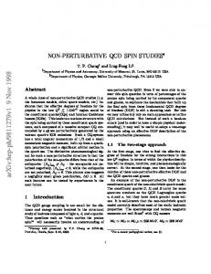
Pictorial representation of a tt¯h event as produced by an event generator. The hard interaction (big red blob) is followed by the decay of both top quarks and the Higgs boson (small red blobs). Additional hard QCD radiation is produced (red) and a secondary interaction takes place (purple blob) before the final state partons hadronise (light green blobs) and hadrons decay (dark green blobs). Photon radiation occurs at any stage (yellow).

Event generation To compare theoretical predictions and experimental events in a detector, there are essentially two different strategies. Either the experimental signature is corrected back to the parton level through “running hadronisation and QCD evolution backwards”, or the full final state is simulated by a computer program including all aspects described above. The former can be viewed as the “experimentalists approach” to validate a given prediction, while the latter is the “phenomenologists approach”. It leads to the construction of computer programs known as event generators. Event generators rely on the factorisation of an event into different stages, corresponding to different energy scales. This is pictorially represented by Fig. 1. In general the simulation starts with the hard process (dark red blob), where perturbation theory is applicable due to correspondingly high scales. This part of the simulation is handled by matrix element (ME) generators. QCD evolution is then run from the hard scale down to the hadronisation scale,

Contents

3

which is of the order of ΛQCD ≈ 1 GeV. This leads to emission of further QCD partons and is handled by shower generators. Partons are now transformed into primary hadrons (light green blobs) through application of a fragmentation model and afterwards decayed into observed particles. A particularly difficult scenario might arise in hadronic collisions, which is depicted by the purple blob in Fig. 1. Remnants of incoming hadrons can themselves undergo a hard or semihard interaction, which then spoils the nice factorisation picture. This effect has been observed experimentally [1] and is addressed in a number of theoretical models [2, 3, 4, 5]. It is commonly referred to as the hard underlying event. Unfortunately, however, a correct quantum mechanical treatment is, at present, out of reach. The most prominent examples of event generators are the well-established PYTHIA [6] and HERWIG [7] programs. They have been constructed over the past decades alongside with experimental discoveries and most of the features visible in past and present experiments can be described through them. However, both the need for higher precision to meet the challenges of new energy scales at the LHC, and the complexity of final states at those scales have demanded those codes to be rewritten in a modern programming language. Object oriented frameworks will then allow to easily implement and test new physics models and potential variants of the old ones. Corresponding efforts led to the construction of the programs PYTHIA 8 [8] and HERWIG ++ [9]. Besides those rewrites, new programs have become available, which aim at a more accurate description of the hard perturbative regime through full next-to-leading order calculations, like MCFM [10]. Also, methods have been proposed for the consistent combination of fixed order corrections with shower programs, describing QCD evolution [11, 12]. Corresponding algorithms are implemented for example in MC@NLO [13] and HERWIG ++ [14]. In some cases, full next-to leading order calculations turn out to be quite cumbersome. Generally difficulties increase even more when going to next-to-next-to-leading order. On the other hand, the major part of real corrections stems from higher order tree-level matrix elements. If the aim is to correctly describe multi-jet topologies, rather than total rates, the preferred choice might be a tool, which takes these effects into account. As the need for better predictions in QCD processes with many particles in the final state has become clear, a substantial activity on developing corresponding techniques and tools has spurred. Several codes are now available that can compute corresponding cross sections and generate events in a fully automatic way. The most prominent examples are certainly ALPGEN [15], HELAC [16], MADGRAPH [17] and AMEGIC++ [18]. However, only AMEGIC++ is part of a fully equipped event generation framework, the SHERPA event generator.

The event generator SHERPA SHERPA [19] is an acronym for Simulation of High Energy Reactions of PArticles. It stands for a fully equipped event generation framework, that has been constructed from scratch and is entirely written in the modern, object oriented programming language C++. It includes the automatic matrix element generator AMEGIC++, the parton cascade APACIC++ [20], a multiple parton interaction module, a fragmentation module [21], a hadron and tau decay library [22] and a program for the simulation of QED radiation [23]. Over the past years, many improvements have been made and many additional features have been included, for example a shower based on Catani-Seymour dipole factorisation [24] and a dipole shower [25]. However, not all of the new features are publicly available yet and in the following, the

4

Contents

default configuration of SHERPA is described. AMEGIC++ is a tree level matrix element generator, based on Feynman diagrams, that is employed for hard matrix element generation throughout SHERPA. It implements a number of interaction models. Besides those for the Standard Model, Feynman rules are included for the MSSM [26], the ADD model [27], effective Higgs couplings to gluons, and others. The generator has been validated in a large number of processes [27, 26]. To evaluate single amplitudes, the helicity methods introduced in Refs. [28] are employed. Feynman diagrams are constructed and sorted according to their respective colour structure. A colour matrix for the full squared matrix element is computed using standard rules. Each single Feynman diagram is then decomposed into basic building blocks in the helicity formalism. The standard phase space integration as realised in AMEGIC++ relies on the factorisation techniques presented in Ref. [29], together with the multi-channel methods introduced in Ref. [30]. Single channels are constructed according to the pole structure of the diagrams leading to the full amplitude and are further refined using adaptive techniques [31]. Other phase space generators, according to Refs. [32, 33] are available. Recently Catani-Seymour dipole subtraction has been automated within AMEGIC++ [34]. QCD parton evolution is accounted for in SHERPA by the program APACIC++. APACIC++ is a standard parton cascade, ordered in virtuality, which implements initial and final state evolution and includes QED radiation effects. QCD coherence is included approximately by imposing an explicit angular veto in subsequent branchings. A particular feature of APACIC++ is that it has been set up for the merging with real next-to-leading order matrix elements, as delivered by AMEGIC++, through the Catani-Krauss-Kuhn-Webber (CKKW) algorithm [35,36]. This approach allows to consistently combine matrix elements of different final state multiplicities with parton showers, while the apparent problem of double counting large logarithmic enhancements is avoided. This has been realised within SHERPA in a fully general way, i.e. no intervention by the user is needed and it can be applied to any QCD associated process. Underlying events are, in the framework of SHERPA, simulated by the AMISIC++ program [37], which implements a model for multiple parton scatterings [2]. This model essentially assumes that the underlying event in hard processes is generated by a sequence of independent hard scatterings, ordered in transverse momentum, which are connected only by the incoming hadrons and common hadronisation of final states. Care must be taken that, when employed in conjunction with the CKKW algorithm, the scale set by the hard process is respected and that it is chosen independent of the final state multiplicity. A corresponding algorithm is implemented into AMISIC++ in full generality. The original model withing PYTHIA has been extended in a similar way at the same time [3] and a model for PDF effects beyond naive rescaling has been incorporated [38]. For the last step of simulation, namely the fragmentation of partons into hadrons and the subsequent hadron decays, SHERPA has long been relying on the Lund string model [39] in the implementation of PYTHIA [40] and the respective decay routines. However, a new type of cluster fragmentation [41] has recently been developed and is now available in the code. It is essentially based on the continuation of a dipole shower model into the nonperturbative region, where the strong coupling is parametrised and can be tuned to better fit the data. The kinematics of cluster splittings into other clusters or hadrons are chosen according to Lorentz invariant evolution parameters. A hadron decay module has recently been completed, which includes a tau decay library and the simulation of all types of mixing effects for neutral mesons.

Contents

5

SHERPA itself is the framework, which puts together all the above and arranges the various phases of event generation. It contains common tool sets and implements the initialisation of the generator as well as the interaction with external software packages through standard interfaces. SHERPA has successfully been employed in experimental analyses [42] and is one of the most advanced new generation simulation programs today.

Motivation for this work Compared to previous experiments, the LHC as next generation collider will pose completely new challenges to both the experimental and the theoretical community. It operates at the highest centre-of-mass energies and provides enormous luminosity. On the experimental side, data acquisition, storage and processing therefore require the creation of a world-wide network for computing needs, the so-called Grid [43]. On the theoretical side, demands for higher precision to correctly model signals and backgrounds of new physics necessitate the construction of modern event generators. As mentioned above, a great challenge in this respect is to correctly simulate production and evolution of QCD partons once they are generated in conjunction with a hard interaction. The correct quantum mechanical treatment of colour has significant impact on the respective results. A proper algorithm for merging matrix elements and parton showers including colour correlations must be incorporated in the simulation. Better shower models are nowadays available, yet it remains to establish the numerical programs for combining them with hard matrix elements. Perturbative QCD computations for large multiplicities need to be carried out in an automated way at tree- and loop-level, which necessitates the refinement of old and construction of new methods for numerics. Corresponding codes must be easy to deploy on the Grid. Modern event generators are not only required to simulate hard QCD processes, however. For example the underlying event might contain semihard or even soft interactions, which are poorly described by perturbative QCD. A related issue is the reggeisation of the gluon and the respective link to the Pomeron, which governs the rise of the total cross section with increasing centre-of-mass energy. Corresponding questions can eventually be addressed at the LHC, leading to new insight about the behaviour of QCD at low scales. Hadronisation and hadron decay models will potentially be refined in the future due to better measurement of related parameters. Better simulation in this area can have significant impact on the understanding of physics at much higher energy scales. In general, modern and flexible event generators are indispensable tools for data analysis. In the near future new and improved simulation programs will therefore replace the well-established traditional ones, allowing a wider range of applicability and more modular frameworks. The key idea is to offer phenomenologists an interface to hadron level events, where new ideas and better theoretical models can easily be implemented such that they can quickly be probed in experiments. At the same time the description of Standard Model backgrounds shall be improved. The construction, validation and extension of event generators is therefore one of the principal tasks of particle physics phenomenology today. This thesis aims at contributing to this field through improving methods for perturbative QCD simulation within the framework of the event generator SHERPA.

6

Contents

Outline of this thesis This thesis is divided into two parts. The first part is concerned with the computation of hard perturbative matrix elements and the efficient sampling of the corresponding phase space. As outlined above, this is one of the key ingredients for any physics simulation through an event generator. The basic formalism for matrix element computation is introduced and recent progress in the field is briefly outlined. A new approach for the recursive computation of QCD and QCD-associated amplitudes is then presented. New methods for phase space sampling are introduced, which allow the simulation of previously inaccessible signatures. A fully general numerical implementation of the corresponding algorithms into the program COMIX [44], within the framework of the SHERPA event generator is presented and results are compared to other high-multiplicity matrix element generators, such as AMEGIC++ and ALPGEN. The second part of the thesis deals with the simulation of DGLAP and BFKL evolution as well as multi-jet-merging procedures. The basic concepts of parton shower generation are presented and the parton cascade APACIC++ is introduced. The CKKW algorithm as a method to systematically include real next-to-leading order corrections through appropriate matrix elements and merging with the parton shower is presented as an example for multijet merging. Improvements and extensions of the original algorithm are discussed, such as a method to incorporate colour information from colour sampled matrix elements. Using different matrix element generators, a comparison is performed for e+ e− -annihilation into hadrons and Drell-Yan lepton pair production. Other merging prescriptions are briefly introduced and a comparison between the results from SHERPA and other generators is presented. Finally a new strategy for the generation of BFKL evolution in a Markovian approach is introduced. The two parts of the thesis are separately summarised. Implications of new or improved techniques of event generation for phenomenology and experiment are outlined and the impact on future event generators is discussed.

Part I Computation of matrix elements

1

Fixed order perturbative QCD

The aim of this section is to introduce techniques for the computation of perturbative QCD tree-level matrix elements at fixed order. The motivation to develop methods beyond the traditional Feynman diagram approach are twofold. Firstly, it turns out that often the final formulae for QCD amplitudes have a much simpler structure than anticipated during intermediate steps of the computation. It might happen that there is even a convenient interpretation of the result, for example in terms of QCD antenna functions [45]. The traditional diagrammatic approach might hide such simplifications or analogies through an unnecessary complicated structure of intermediate terms. It is worthwhile to circumvent these complications, if possible. For example it turns out that many analytical perturbative QCD computations are greatly alleviated using novel techniques like the Britto-CachazoFeng (BCF) on-shell recursion discussed below. Secondly, one might gain additional insight into the underlying structure of perturbative QCD through techniques which yield results that are simple and easy to interpret. For example soft and collinear factorisation properties of QCD tree amplitudes can be understood in a very convenient way through the CSW technique [46, 47]. On the other hand it turns out that many of the newly emerging methods are very suited to solve a particular physical problem only, like for example the computation of a scattering amplitude in a certain helicity assignment of external particles. They can of course be invoked to yield results for the full theory, but in practice “old fashioned” methods are often much more suited for the task and more generally applicable. Which technique to compute QCD scattering amplitudes is employed, thus depends very much on the purpose of the computation itself. Whenever an analytical result is desired, one would rather focus on methods that yield the most compact analytical expressions and not care about their numerical evaluation. A popular example for this is the colour-dressed BCF recursion relation, presented in Ref. [48], which has a stunningly simple form. On the other hand, it leads to a factorial proliferation of terms, once a result must be computed numerically. Therefore, whenever the aim is the numerical evaluation of amplitudes and thus the computation of physical cross sections, the focus will be on the simplest implementation in terms of computer algebra and the best algorithmic choice to save computation time. At this point it is mostly found that traditional recursive methods to compute scattering amplitudes are the better alternatives [49, 48, 50]. The outline of this chapter is as follows. Firstly various methods to separate the amplitude computation into colour factors and the computation of planar diagrams are introduced. This point is crucial for both the basic CSW and the basic BCF relations. In Chapter 2, it will be shown how to reinstate colour information in the computation. Secondly, the Weyl-van der Waerden formalism to compute helicity amplitudes is reviewed, since it is one of the basic ingredients for the discussions in the following chapters. It is outlined how the analytical computation of tree-level amplitudes is performed in this method. Maximally

10

1 Fixed order perturbative QCD

helicity violating (MHV) amplitudes, which will be essential for the discussion of the CSW and the BCF relations, are derived. The Berends-Giele (BG), CSW and BCF relations are presented.

1.1

Colour Decompositions

In this section the method of colour decomposition is briefly outlined and the available results for tree-level QCD amplitudes with n gluons are presented as an example. Emphasis is given to those aspects which will play an important role in the following chapters. The basic idea of a colour decomposition is to factorise the information on the gauge structure from the kinematics. Results are mostly formulated for an arbitrary number of colours NC . This allows, for example in the context of a parton shower picture, cf. Part II, Chapter 1, to interpret results in the large NC limit. In this context, quarks may thus carry a fundamental colour index i = 1, . . . , NC , antiquarks carry a fundamental “anticolour” index ¯ = 1, . . . , NC and gluons usually carry an adjoint colour index a = 1, . . . , NC2 − 1. The fundamental interaction between quarks and gluons is mediated by a term proportional Ti¯a , T being the generators of SU(N) in the fundamental representation. Gluons couple through f abc , with f the being the structure constants of SU(N). In the notation employed here, T ’s are normalised according to Ti¯a T¯bi = δ ab ,

(1.1)

which allows some simplification in further computations. Structure constants are defined through a b (1.2) T , T i¯ = i f abc Ti¯c .

This definition immediately yields the relation f abc Tr T c , T d1 , T d2 , . . . T dn−1 , T dn . . . = , − i Tr T a , T b , T d1 , . . . T dn−1 , T dn . . .

(1.3)

which can be employed to rewrite a string of structure constants in terms of fundamental representation matrices. As an example, consider the amplitude A for n gluons of colours a1 , a2 , . . . , an . Using Eq. (1.3) one can prove that, at tree level, such an amplitude can be decomposed as [51] X Tr [ T a1 T aσ2 . . . T aσn ] A(1, σ2 , . . . , σn ) , (1.4) A(1, . . . , n) = σ∈Sn−1

where the sum is over all (n − 1)! permutations of (2, . . . , n). Each trace corresponds to a particular colour structure. The factor associated with each colour structure, A, is called a colour-ordered amplitude. It is also referred to as a dual amplitude or partial amplitude. It depends on the four-momenta pi and polarisation vectors εi of the n gluons, represented simply by the particle index in its argument. The colour-ordered amplitudes are far simpler to calculate than the full amplitude A, since they contain only planar graphs and thus a much smaller number of Feynman diagrams contribute to them. They also have remarkable theoretical properties. Among those, a special role is played by the Kleiss-Kuijf

1.1 Colour Decompositions

11

relations [52]. These are linear relations amongst the amplitudes directly inherited from the gauge structure, i.e., from colour, which in the case of n-gluon amplitudes reduce the number of linearly-independent amplitudes to (n − 2)!. It is then clear that the number of terms in Eq. (1.4) cannot be minimal. This decomposition is, however neither unique nor special and other colour decompositions might be more suited for a particular problem. Eq. (1.4) is universally used to illustrate the idea of colour decompositions and to define the full amplitude A in terms of colour-ordered amplitudes A. It can be shown, however, that the above definition of colour-ordered amplitudes does not depend on the actual colour basis. Recently, another decomposition has been introduced, which is based on colour flows [16,53]. This decomposition arises when treating the SU(N) gluon field as an NC ×NC matrix (Aµ )i¯ (i, ¯ = 1, . . . , NC ), rather than as a one-index field Aaµ . To understand why this might be helpful, consider the term Ti¯a Tka¯l , corresponding to the sum of all gluons propagating between two quark lines, i.e. the gluon propagator. This term can be decomposed as Ti¯a Tka¯l = δi¯l δk¯ −

1 δi¯ δk¯l NC

↔

¯

k

i

¯l

−

1 NC

¯

k

i

¯l

.

(1.5)

Regarding these two terms, it becomes apparent why the basis for this decomposition is called the colour-flow basis. Both terms correspond to connecting indices of fundamental SU(N) objects. Their sum gives a projection which exactly yields the NC2 −1 degrees of freedom of the gluon field. Correspondingly, the elementary quark-gluon vertex is proportional to delta functions connecting the gluon and quark lines and quark lines are simple delta functions. Gauge couplings have a more complicated structure, which will be explained in detail in Chapter 2. The major advantage of this decomposition is that any colour factor can be decomposed into a product of delta functions. This allows a straightforward implementation into computer programs, since no matrix multiplications of complex valued matrices have to be performed, but only integer comparisons. Corresponding codes are therefore often much faster, even if the natural colour basis is not the colour-flow basis and therefore the number of terms in the sum over permutations is not minimal. This will be discussed in more detail in Chapter 2. Within the colour-flow basis, the n-gluon amplitude may be decomposed as X ¯σ ¯σ δi1 2 δiσ23 · · · δi¯σ1n A(1, σ2 , . . . , σn ) , A(1, . . . , n) = (1.6) σ∈Sn−1

where the sum is over all (n − 1)! permutations of (2, . . . , n). The partial amplitudes that appear in this decomposition are the same as in the decomposition in the fundamental representation. As can be seen here, another nice feature of the colour-flow decomposition is that the colour factors in front of each amplitude are either zero or one. A similar decomposition exists for all tree-level parton amplitudes including any number of quark pairs, gluons and colour singlet objects. A third decomposition of the multi-gluon amplitude exists, which is based on the adjoint representation of SU(N) rather than the fundamental representation [54]. It can be inferred from Eq. (1.3) using (F a2 F a3 · · · F an−1 )a1 an = Tr ( T a1 , [ T a2 , . . . [ T an−1 , T an ] . . . ] ) ,

(1.7)

12


where (F a )bc = −if abc are the adjoint-representation matrices of SU(N). The n-gluon amplitude in this decomposition may be written as X (F aσ2 F aσ3 · · · F aσn−1 )a1 an A(1, σ2 , . . . , σn−1 , n) , A(1, . . . , n) = (1.8) σ∈Sn−2

where the sum is over all (n − 2)! permutations of (2, . . . , n − 1). The indices corresponding to the first and the last gluon are taken as “references” and are not included in the permutations. The partial amplitudes that appear in this decomposition are the same as in the other decomposition, but only (n − 2)! linearly-independent amplitudes are needed. In this respect this formulation is “minimal” as there is no redundancy and the Kleiss-Kuijf relations are embodied in the colour factors. As will be elaborated upon in Chapter 2, there exists a remarkable formal similarity with the BCF recursive relations, where two gluons are also taken as a reference to build up the full amplitude.

1.2

The Weyl-van der Waerden spinor formalism

In this section a brief introduction to the spinor formalism employed in the computation of helicity amplitudes is presented. The discussion closely follows Refs. [55, 56], where the algorithm was introduced in great detail. The focus will be on massless fermions and gauge particles, however masses can be introduced, for example in the formalism presented in Ref. [57]. This will be discussed in Chapter 3. Although solutions to the Dirac and Maxwell equations are in principle known, the actual implementation in a given computation can be quite cumbersome. If an inconvenient spinor basis or unsuitable polarisation vectors are chosen, the computation can be unnecessarily complicated. A convenient way to define spinors is to employ the Weyl-van der Waerden formalism [58].

The basic formalism Spinors in the D( 21 , 0) and D(0, 21 ) representation of the Lorentz group are called rightand left-handed Weyl spinors, respectively. They are defined through dotted and undotted spinor indices, such that ψa is a covariant (right-handed) and ψ a˙ is a contravariant (lefthanded) spinor. Complex conjugation amounts to dotting and undotting indices, according to ∗ ψa˙ = (ψa )∗ , ψ a = ψ a˙ . (1.9)

Spinor indices are lowered and raised using the spinor metric, given in terms of the ε tensor 0 1 ab a˙ b˙ . (1.10) ǫ = ǫ = ǫab = ǫa˙ b˙ = −1 0

To compute polarisation vectors and to describe the fundamental interactions between vectors and fermions, the matrices σ µ are defined. They allow to decompose a four-vector, which is an object of the D( 12 , 12 ) representation of the Lorentz group in terms of two spinors. ˙ (1.11) σ µ ab = σ 0 , ~σ , σ µab˙ = σ 0 , −~σ ,

1.2 Weyl-van der Waerden formalism

13

where σ 0 = I is the 2 × 2 unit matrix and ~σ are the Pauli matrices. Using these definitions, an arbitrary real four vector k µ can be rewritten as a 2 × 2 matrix + k± = k0 ± k3 k k⊥ µ . (1.12) , where kab k = ˙ = σab µ ∗ ˙ k⊥ = k 1 + ik 2 k⊥ k− 2 For massless vectors, one has ~k⊥ = k + k − and therefore a spinor ξ(k) can be determined such that kab ˙ = ξa˙ ξb . √ k+ √ kab where ξa (k) = , φk = arg k⊥ . (1.13) ˙ = ξa˙ (k) ξb (k) , k − eiφk µ a˙ b Employing the definition of σ µ , Eq. (1.11) again, conversely one obtains 2k µ = σab ˙ ξ ξ . Note that the above definition of ξ is not unique. Firstly, an arbitrary phase can be multiplied without changing the result. Secondly, Eq. (1.12) is ambiguous itself, because the x-, y- and z-direction along which k⊥ and k ± are defined can be changed through a rotation of the Pauli matrices. This can be referred to as the spinor gauge and the actual definition of the Pauli matrices as the preferred basis amounts to a gauge fixing. In order to obtain the decomposition of a massive vector in terms of the above defined Weyl spinors, it is customary to employ the following decomposition of a massive four vector into massless ones

k µ = bµ − κaµ ,

where

κ =

k2 . 2 ak

(1.14)

In this respect, aµ is an arbitrary light-like four-vector. Selecting a certain aµ amounts to a gauge choice for the decomposition. According to the above formulae, one obtains kµ =

1 µ a˙ b κ µ a˙ b σ ˙ b b − σab a a . 2 ab 2 ˙

(1.15)

It is convenient to define the inner products in spinor space through hξηi = ξa η a ,

[ξη] = ξa˙ η a˙ ,

(1.16)

which immediately yields the relation [ξη] = hξηi∗. Due to the spinor metric ǫ, the inner product is antisymmetric in its arguments and the Schouten identity holds hφψihξηi + hφξihηψi + hφηihψξi = 0 .

(1.17)

For further computations, a shorthand notation is introduced which denotes the spinor ξa (ki) determined from a massless four vector ki through Eq. (1.13) as |kii or |ii and the ˙ corresponding ξ a˙ (ki ) as |ki] or |i]. In full analogy [i|σ µ |ji = σ µ ab ξa˙ (ki )ξb (kj ). The invariant mass of a pair of massless particles described by the four vectors ki and kj is then given by 2 ki kj =

1 [i|σ µ |ii[j|σµ |ji = hiji [ji] . 2

(1.18)

Thus it can be seen that the spinor products are, up to a phase, square roots of Lorentz invariants. It is known that the final result for the squared amplitude will be directly expressible in terms of Lorentz invariants. Therefore all unphysical phases occurring due to gauge choices in the spinor products must cancel, which can be employed as a consistency check of the calculation.

14


Wave functions for helicity eigenstates In this subsection, explicit Dirac spinors and polarisation vectors will be constructed employing the Weyl-van der Waerden formalism. A Dirac spinor belongs to the D( 21 , 0) ⊕ D(0, 21 ) representation of the Lorentz group and can be represented in terms of Weyl spinors as a˙ φ . (1.19) Ψ = ψa The corresponding Dirac matrices read ˙ 0 σ µ ab −σ 0 0 5 0 1 2 3 µ . , γ = iγ γ γ γ = γ = 0 σaµb˙ 0 σ0

(1.20)

Covariant and contravariant spinors ψa and φa˙ can be singled out using the projectors PR,L = P± =

1 ± γ5 . 2

(1.21)

The Dirac equation for a particle of mass m and four-momentum pµ can be solved by employing the plane wave solutions Ψ = exp {±ikx} Ψ± (k), which leads to the following Eigenspinor problem   −m 0 p− −p∗⊥  0 −m −p⊥ p+  u . (1.22) 0 = (pµ γµ − m) u =   p+ p∗⊥ −m 0  p⊥ p− 0 −m p Eigenvalues are λ = m ± p2 . Defining the variables p¯ = sgn (p0 ) |~p | and pˆ = ( p¯, ~p ), a possible set of Eigenspinors is given by [57] √ √ 1 1 p0 − p¯ χ+ (ˆ p) p) − p0 − p¯ χ+ (ˆ √ √ , v− (p, m) = √ , u+ (p, m) = √ p0 + p¯ χ+ (ˆ p) p0 + p¯ χ+ (ˆ p) 2 p¯ 2 p¯ (1.23) √ √ 1 1 p0 + p¯ χ− (ˆ p) p0 + p¯ χ− (ˆ p) √ √ , v+ (p, m) = √ . u− (p, m) = √ p0 − p¯ χ− (ˆ p) p) 2 p¯ 2 p¯ − p0 − p¯ χ− (ˆ The above definition has the apparent advantage, that massless spinors have two nonzero components only. This, together with Eqs. (1.20) greatly simplifies the computation for massless theories. The Weyl spinors χ± (p) read + √ 1 pˆ pˆ+ √ χ+ (ˆ p) = √ + = pˆ⊥ pˆ− eiφpˆ pˆ √ (1.24) eiπ pˆ−√e−iφpˆ −ˆ p∗⊥ . = χ− (ˆ p) = √ + − pˆ+ pˆ+ pˆ They are orthogonal and normalised to 2 |ˆ p0 |. The Eigenspinors u± and v± are thus orthogonal and normalised to 2m and −2m, respectively. In the following, the notation of Ref. [55] is adopted and massless Dirac spinors are also denoted using u± (k) = v∓ (k) = |k ± i ,

u¯± (k) = v¯∓ (k) = hk ± | .

(1.25)

1.2 Weyl-van der Waerden formalism

15

Polarisation vectors for external vector bosons are constructed according to Ref. [56]. For massless gauge bosons the wave function V µ satisfies Maxwell’s equations and the Ansatz V µ = exp {−ikx} εµ± (k) can be made. One possible set of polarisation vectors is then given by hk ∓ |γ µ |p∓ i εµ± (p, k) = ± √ . 2 hk ∓ |p± i

(1.26)

In this context, k is an arbitrary light-like gauge vector, which must not be parallel to the momentum p. The above definition yields the polarisation sum of a light-like axial gauge X

λ=±

εµλ (k, p)ενλ ∗ (k, p) = −g µν +

k µ pν + k ν pµ . kp

(1.27)

For massive vector bosons the wave function must satisfy Proca’s equation and one obtains one additional polarisation hk ∓ |γ µ |b∓ i εµ± (p, k) = ± √ , 2 hk ∓ |b± i

εµ0 (p, k) =

1 hb− |γ µ |b− i − κhk − |γ µ |k − i , m

(1.28)

where, as introduced above, b = p − κk and κ = p2 /2pk. Again k is an arbitrary light-like gauge vector. The polarisation sum is however independent of k and reads X

λ=±,0

εµλ (k, p)ενλ ∗ (k, p) = −g µν +

pµ pν . p2

(1.29)

Note that the computation of terms like in Eq. (1.28) can be simplified by using the identities hk + |γ µ |p+ i = [k|σ µ |pi , hk − |γ µ |p− i = hk|σ µ |p] ,

hk − |p+ i = hkpi , hk + |p− i = [kp] .

(1.30)

Equation (1.30) implies that for massless QCD, the two component Weyl-van der Waerden spinors are sufficient to compute any given scattering amplitude.

Connection to the helicity formalism Another formalism to compute helicity amplitudes, based only on Lorentz invariants has been presented in Refs. [28]. It is the basis for many modern matrix element generators, like for example AMEGIC++ and MADGRAPH. The Weyl-van der Waerden formalism can easily be translated into this helicity formalism, since only the redundant phase information encoded in the spinor products must be eliminated. Within the Weyl-van der Waerden formalism, the following relations hold |i± ihi± | =

1 ± γ5 k/i . 2

(1.31)

This is, however exactly the relation which defines the basic spinors within the helicity formalism, cf. Refs. [28] and therefore the connection is immediately established. Another, more convenient way to understand the relation between the two methods was presented in Ref. [55]. A brief summary of the arguments discussed ibidem is given in the following.

16


Within the full scattering amplitude, any spinor string must terminate, since otherwise the dependence on unphysical phases introduced by the gauge choices described above cannot be eliminated. Such a string has the form hi1 i2 i [i2 i3 ] hi3 i4 i . . . hi2n i1 i .

(1.32)

The question is, whether there is a general method to reduce the string to minimal pieces and what these pieces look like. A solution to the problem is obtained if one realises that 1 = hiji [ji] /2 kikj . Multiple insertions of this relation will yield strings of maximum length four, which can easily be evaluated. If its length is two, the string will simply be a scalar product. If its length is four, with the help of Eq. (1.31) and the Fierz rearrangement hi− |γ µ |j − ihk − |γµ |l− i = −2 hiki [jl] ,

(1.33)

one obtains 1 − µ − − hi |γ |j ihj |γµ |l− ihl− |γ ν |n− ihn− |γν |i− i 4 1 − γ5 = Tr k/i k/j k/l k/n 2 = 2 ki kj kl kn − ki kl kj kn + ki kn kj kl − iǫµνρσ kiµ kjν klρ knσ .

hiji [jl] hlni [ni] =

(1.34)

Up to a normalisation factor and with a proper choice of vectors, this is exactly the Sfunction of the helicity formalism, as defined in Ref. [28]. If k0 and k1 are the gauge vectors with k0 k1 = 0, and p1 and p2 the vectors of Dirac particles, the corresponding S-functions in terms of Weyl-van der Waerden spinors read hp1 p2 i [p2 k0 ] hk0 k1 i [k1 p1 ] √ 4 p1 k 0 p2 k 0 [p1 p2 ] hp2 k0 i [k0 k1 ] hk1 p1 i √ S(−; p1 , p2 ; k0 , k1 ) = 4 p1 k 0 p2 k 0 S(+; p1 , p2 ; k0 , k1 ) =

(1.35)

Equation (1.34) can be employed to transform results obtained with the the two different methods into each other.

1.3

The Berends-Giele recursive relations

In Ref. [59], Berends and Giele introduced the colour-ordered n-point gluon off-shell current J µ , which can be defined as the sum of all colour-ordered Feynman diagrams with n external on-shell legs and a single off-shell leg with polarisation µ. The colour-ordered off-shell currents can then be constructed using the Berends-Giele recursive relations ( n−1 X µνρ −i V (P1,k , Pk+1,n ) Jν (1, . . . , k)Jρ (k + 1, . . . , n) J µ (1, 2, . . . , n) = 2 P1,n k=1 3 ) (1.36) n−2 X n−1 X V4µνρσ Jν (1, . . . , j)Jρ (j + 1, . . . , k)Jσ (k + 1, . . . , n) , + j=1 k=j+1

1.3 Berends-Giele recursion

17

1 2 J

µ

1 2

1 2

= n−1 n

n−1 X

i+1

i−1 i

V3

+

i=2

i+1 i+2

n−2 X

i+2

V4

i=2 j>i

n n−1

Fig. 1.1

i−1 i

j−1 j n

n−1

j+2 j+1

Pictorial representation of the Berends-Giele recursive relations, Eq. (1.36)

where the momentum sum Pi,j is defined through Pi,j =

j−1 X

pk ,

(1.37)

k=i

and where V3µνρ (P1,k , Pk+1,n ) and V4µνρσ are the colour-ordered three and four-gluon vertices defined in Ref. [55]. gs νρ µνρ µ ρµ ν µν ρ √ V3 (P, Q) = i , g (P − Q) + 2g Q − 2g P 2 (1.38) gs2 µρ νσ µνρσ µν ρσ µσ νρ V4 =i . 2g g − g g − g g 2 The algorithm is schematically depicted in Fig. 1.1. A full n+ 1-gluon amplitude is obtained by amputating the off-shell propagator and contracting the remaining quantity with the external polarisation of gluon n + 1. A(1, . . . , n + 1) =

2 P1,n µ εn+1

i

Jµ (1, . . . , n) .

(1.39)

Similar recursions exists for the off-shell quark currents [59]. For some exceptional cases Eq. (1.36) can be solved in closed form [59, 60]. In particular one obtains the n-gluon off-shell current with like-sign helicity gluons J µ (1+ , . . . , n+ ) = gsn−2 √

hk − |γ µP/1,n |k + i . 2hk1ih12i . . . hn−1 nihnki

(1.40)

It can be used to prove the form of maximally helicity violating (MHV) or Parke-Taylor tree amplitudes, which was first conjectured by Parke and Taylor in Ref. [61] and proved by Berends and Giele in Ref. [59]. Such amplitudes correspond to the “mostly plus” (“mostly minus”) helicity assignment, where only two of n gluons have negative (positive) helicity. They are given by the simple formulae hiji4 , h12i . . . hn−1 nihn1i [ij]4 − + + − n−2 . A(1 , . . . , i , . . . , j , . . . , n ) = i gs [12] . . . [n−1 n] [n1] A(1+ , . . . , i− , . . . , j − , . . . , n+ ) = i gsn−2

(1.41)

18


The applicability of Berends-Giele type recursive relations in analytical calculations is somewhat limited due to the explicit occurrence of four-vectors and polarisations. For this reason, however they allow a straightforward implementation into computer programs and are hence particularly suited for numerical analysis. In Chapter 3, the concept of Berends-Giele type recursive relations will therefore be extended to the full Standard Model.

1.4

The CSW vertex rules

The aim of this section is to introduce the CSW vertex rules, which are one of the major theoretical improvements in the understanding of perturbative QCD in recent years. In this respect, unexpected progress has come from twistor-inspired methods [62], which have provided new techniques to compute analytic results for gauge amplitudes both at tree and one-loop level [63]. These new methods go back to a correspondence between a weakly coupled N = 4 Super Yang-Mills theory and a certain type of string theory. The key point in this correspondence is that all tree-level colour-ordered amplitudes are related to algebraic curves in twistor space. In Ref. [64] it was shown that this leads to the CSW vertex rules. These rules state that it is possible to build arbitrary colour-ordered amplitudes from MHV amplitudes, which, in this context will also be referred to as MHV vertices [62,63,64]. These “elementary” vertices are connected by scalar propagators, thus eventually building up a full n-gluon amplitude with n − l like-sign helicity gluons through l − 1 MHV amplitudes. Each off-shell leg with momentum P then corresponds to a spinor Paa˙ η a˙ , using some arbitrary contravariant reference spinor η a˙ . The CSW rules for constructing an arbitrary n-gluon colour-ordered amplitude are 1. For n − l like-sign helicity gluons, draw all possible graphs connecting l − 1 MHV vertices. In this context the 3-gluon MHV vertex must be included, since intermediate particles are off-shell and therefore the 3-gluon MHV amplitude does not vanish. 2. While maintaining their cyclic ordering, match the n external indices onto the above defined graphs, respecting the helicity assignment of the gluons. Typically this will eliminate a number of possible graphs. This procedure is exemplified in Fig. 1.2, where all MHV graphs contributing to the 6-gluon amplitude A(−, −, −, +, +, +) are shown. The algorithm can be reformulated such that only skeleton graphs containing the external legs with opposite sign helicity have to be drawn, while the like-sign helicity legs are distributed along the vertices as needed. In this context, only a single skeleton graph contributes to any non-MHV six-gluon amplitude. The CSW rules imply that an n-point colour-ordered amplitude may have contributions from MHV vertices involving up to n particles. The number of different vertices is thus growing steadily with the number of particles, which makes it impossible to put for example Berends-Giele recursive relations and the CSW rules on the same footing. This problem has also been addressed in Ref. [65] and will be dealt with in Chapter 2, where it is shown how the CSW vertex rules can be rewritten in a truly recursive fashion.

1.5 BCF recursion

19

2−

5+

1−

+ −

6+

3−

4+

4+

3−

5+

+ −

+ −

3− 4+ 5+

4+ 3− 2−

+ −

3− + −

1−

1.5

5+ 6+ 1− 4+

4+

3−

5+

2−

+ −

6+ Fig. 1.2

1−

2−

2− 1− 6+

2−

6+

5+ 6+ 1−

The six MHV graphs for the computation of the 6-gluon non-MHV amplitude A(−, −, −, +, +, +) in the CSW formalism. Gluons are represented by straight lines, while grey blobs denote MHV amplitudes.

The BCF recursive relations

In this section, the BCF recursive relations, presented in Refs. [66] shall be introduced. Like the CSW vertex rules presented above, they are an outcome of major theoretical improvements in the calculation of higher order QCD corrections. They state that any treelevel colour-ordered amplitude can be constructed from products of two on-shell amplitudes of fewer particles, multiplied by a simple scalar propagator. These new calculational tools have allowed to derive expressions for multi-parton amplitudes [67], which have simple and compact analytic forms. Assuming an n-gluon amplitude with 1 and n being opposite sign helicity gluons, the BCF recursive relations read An (1, 2, . . . , n) =

n−2 X k=2

1 h −h ˆ ˆ 2, . . . , k, −Pˆ1,k A P , k + 1, . . . , n ˆ , Ak+1 1, n−k+1 1,k 2 P1,k

(1.42)

where a sum over the helicities h of the intermediate gluon is implicit, and ˜1 , Pˆ1,k = P1,k + zλn λ ˜1 , pˆ1 = p1 + zλn λ

(1.43)

˜1 . pˆn = pn − zλn λ ˜ i are the co- and contravariant spinor components of the light-like In this context λi and λ

20


2

n−2 n−1

3

=

An

n−2 X X

n

i+1 i+2 n−2

i−1 i

Ak+1

i=2 h=±

1 Fig. 1.3

2

3

ˆ ∓h ∓P 1,i

n−1

An−k+1

ˆ1

n ˆ

Pictorial representation of the BCF recursive relations, Eq. (1.42).

˙

˙

˜ b . The shift parameter z is defined through momenta pai b = λai λ i z =

2 P1,k . hn|P1,k |1]

(1.44)

The last two lines of Eq. (1.43) correspond to shifting the co- and contravariant components of p1 and pn , respectively. It is easily seen that pˆ1 and pˆn still have a factorised form and are therefore complex valued light-like vectors. This is in contrast to the CSW vertex rules, where intermediate gluon lines are off-shell. The subamplitudes in the BCF recursion are, however still not gauge invariant objects. Namely, the choice of reference opposite sign helicity gluons corresponds to a gauge choice, which enters the subamplitudes through dependence on the shift parameter z. Similar recursive relations exist for amplitudes with quarks and for QED processes. Equation (1.42) is schematically depicted in Fig. 1.3.

2

Colour dressed recursive relations for QCD

So far, many extensions of the twistor-inspired methods introduced in Chapter 1 have been constructed, in particular generalisations to include scalars [68], fermions [69] and photons [70]. In this chapter another new extension of the CSW and BCF techniques is presented. It is shown that it is possible to reformulate the twistor-inspired recursive relations for the colour-ordered amplitudes in terms of full amplitudes. The motivations are twofold. The first is mostly theoretical and stems from the observation of an interesting similarity between the colour decomposition Eq. (1.8), based on the adjoint representation, and the BCF recursive relations which suggested the existence of a formulation that embodies both. The second is more pragmatic and aims at establishing whether the new twistor-inspired recursive relations are an improvement also at the numerical level. In order to make a consistent comparison with the most efficient algorithms available [15,71], a recursive formulation which includes colour is necessary. In the standard approach where the colour-ordered amplitudes are calculated analytically (or numerically), one has to sum over the permutations of the colour orderings to obtain the full amplitude. This algorithm has an intrinsic factorial growth and cannot compete with the available numerical methods which only grow exponentially. In this chapter a general method to reinstate colour into the recursive relations for colour-ordered amplitudes is derived and applied to the BCF and to a modified version of the CSW relations. This chapter is organised as follows. In Sec. 2.1 a simple derivation of the colour-dressed counterpart of the Berends-Giele recursive relations is presented, which serves as an illustration of the method that will be applied later. In Section (2.2) the CSW vertex rules are reformulated in terms of simple new three-point effective vertices and the corresponding colour-dressed version is derived. In Sec. 2.3 one of the main results is proved, which is the colour-dressed version of the BCF relations, Eq. (2.43). Its most important features are discussed. Section 2.4 contains numerical results on the evaluation of multi-gluon amplitudes obtained using the different colour-dressed recursive relations, focusing on the comparison with known techniques.

2.1

Colour dressed Berends-Giele relations

Upon inspecting Eq. (1.36) it is easy to see that the four-gluon vertex appearing in the Berends-Giele recursive relations introduces a larger number of possible combinations of subcurrents than the three-gluon vertex. It is however possible to simplify the recursion by decomposing all four-gluon vertices into three-vertices including a tensor particle. This is schematically depicted in Fig. 2.1. Using this decomposition, the Berends-Giele recursive

22

2 Colour dressed recursive relations for QCD

+

= Fig. 2.1

Diagrammatic representation of the decomposition of the colour-ordered fourgluon vertex.

relations can be rewritten such that only three-point vertices are present ( n−1 X −i J µ (1, 2, . . . , n) = 2 V3µνρ (P1,k , Pk+1,n ) Jν (1, . . . , k)Jρ (k + 1, . . . , n) P1,n k=1 +

VTνµαβ Jν (1, . . . , k)Jαβ (k

+ 1, . . . , n) +

VTµσαβ Jαβ (1, . . . , k)Jσ (k

+ 1, . . . , n)

)

(2.1) ,

where Jαβ is a tensor off-shell current, and VTµναβ is the tensor-gluon vertex, defined as VTµνρσ =

ig µρ νσ (g g − g µσ g νρ ) . 2

(2.2)

As there exists no one-point tensor off-shell current, all such currents appearing in Eq. (2.1) are defined as zero. The tensor off-shell currents can be easily constructed recursively from gluon off-shell currents Jµν (1, 2, . . . , n) =

iDµναβ VTσραβ

n−1 X

Jρ (1, . . . , k)Jσ (k + 1, . . . , n),

(2.3)

k=1

where iDµναβ is the colour-ordered tensor “propagator”, defined as i iDµνρσ = − (g µρ g νσ − g µσ g νρ ) . 2

(2.4)

A systematic method to dress colour-ordered recursive relations with colour is now presented in order to obtain recursive relations for the colour-dressed off-shell currents. In the colourflow decomposition, a colour-dressed gluon off-shell current can be written as X ¯ ¯σ ¯ (2.5) δiJσ1 δiσ21 . . . δIσn J µ (σ1 , σ2 , . . . , σn ), JIµJ¯(1, 2, . . . , n) = σ∈Sn

¯ is the colour of the off-shell leg. A colour-dressed tensor off-shell current can where (I, J) be obtained similarly. During the colour dressing of the Berends-Giele recursive relations, Eq. (2.1), the pure gluon vertices and the tensor-gluon vertices can be dealt with separately. After inserting Eq. (2.1), into the colour-flow decomposition, Eq. (2.5), the three-gluon vertex part reads n−1 −i X X J¯ ¯σ1 ¯ δiσ1 δiσ2 . . . δIσn V3µνρ Pσ1 ,σk , Pσk+1 ,σn Jν (σ1 , . . . , σk )Jρ (σk+1 , . . . , σn ), 2 P1,n σ∈S k=1 n

(2.6)

2.1 Colour dressed Berends-Giele relations

23

L J¯ I

J¯ I

Jµ

Jν

¯ L ¯ K

K

¯ G G ¯ H H N ¯ ¯ N M M

Jρ Diagrammatic representation of the decomposition Eq. (2.8) of the colour factor of the three-gluon vertex part.

Fig. 2.2

where Pσ1 ,σk = pσ1 + pσ2 + . . . + pσk , Pσk+1 ,σn = pσk+1 + pσk+2 + . . . + pσn .

(2.7)

The colour factor appearing in Eq. (2.6) can be written as (cf. Fig. 2.2) ¯

¯

¯

¯

¯

J H δI δiJσ1 δiσσ21 . . . δIσn = δG

¯

¯

¯

K M δH δLG δN

¯

¯σ

δiLσ1 . . . δK k

¯

δiNσ

¯

k+1

. . . δMσn ,

(2.8)

where ¯

¯

J H δI is the colour structure of the propagator appearing in the Berends-Giele recursive - δG relations. ¯σ

¯

- δiLσ1 . . . δK k is the colour structure of the subcurrent Jν (σ1 , . . . , σk ), where the off-shell ¯ leg ν has colour (K, L). ¯

¯

- δiNσ . . . δMσn is the colour structure of the subcurrent Jρ (σk+1 , . . . , σn ), where the offk+1 ¯ ). shell leg ρ has colour (M, N ¯

¯

¯

K M δH is part of the colour structure of a three-gluon vertex to which the off-shell - δLG δN ¯ (K, L), ¯ (M, N) ¯ are attached. legs µ, ν, ρ with colours (G, H),

An ordered partition of a set E into two independent parts is now defined as a pair (π1 , π2 ) of subsets of E such that π1 ⊕ π2 = E, which means (π1 , π2 ) 6= (π2 , π1 ). Furthermore, an (unordered) partition of a set E into two independent parts is a set {π1 , π2 } of subsets of E such that π1 ⊕ π2 = E and {π1 , π2 } = {π2 , π1 }. These definitions can easily be extended to partitions of a set E into n > 2 independent parts, for both the ordered and the unordered case. In the case encountered here E = {1, 2, . . . , n}. The set of all ordered partitions of E into two independent parts will be denoted by OP (n, 2), while the set of all (unordered)

24


partitions of E into two independent parts is denoted by P (n, 2). Using these definitions, the sum over permutations appearing in Eq. (2.6) can be decomposed as follows: For a given value of k, - Choose an ordered partition π = (π1 , π2 ) in OP (n, 2) such that #π1 = k, where #π1 is the number of elements in the set π1 . - Fix the first k elements of the permutation to be in the subset π1 . - Sum over all permutations of the first k elements and over all permutations of the last n − k elements. - Sum over all possible choices for the ordered partition π = (π1 , π2 ). This is equivalent to the replacement n−1 X X

k=1 σ∈Sn

→

X

X

X

σ′ ∈S

π∈OP (n,2) σ∈Sk

.

(2.9)

n−k

The three-gluon vertex part now reads ¯ J¯ H δI δG

−i 2 P1,n ¯ δiLσ

¯ ¯ M ¯ K δH δLG δN

V3µνρ

π∈OP (n,2) σ∈Sk σ′ ∈Sn−k ¯σ

π1

X X

X

πk

. . . δK Jν (σπ1 , . . . , σπk )

¯ δiNσ′

π k+1

Pσπ1 ,σπk , Pσ′ k+1 ,σπ′ n π

¯σ ′

(2.10)

. . . δM Jρ (σπ′ k+1 , . . . , σπ′ n ), πn

where π1 = {π 1 , π 2 . . . , π k } and π2 = {π k+1 , π k+2, . . . , π n }. Clearly, Pσπ1 ,σπk and Pσ′ k+1 ,σπ′ n only depend on the choice of the ordered partition π = π (π1 , π2 ), but not on the order of the elements in π1 and π2 . Therefore one can define P π 1 = pπ 1 + pπ 2 + . . . + pπ k , Pπ2 = pπk+1 + pπk+2 + . . . + pπn .

(2.11)

It is now possible to identify several subcurrents in this expression, namely X ¯ ¯σ ¯ δiLσ 1 . . . δK πk Jν (σπ1 , . . . , σπk ), JνK L (π1 ) = π

σ∈Sk

¯

JρM N (π2 ) =

X

¯σ ′

¯

δiNσ′

π k+1

σ′ ∈Sn−k

. . . δMπn Jρ (σπ′ k+1 , . . . , σπ′ n ),

(2.12)

such that the three-gluon vertex part reads ¯

¯

J H δI δG

−i 2 P1,n

X

π∈OP (n,2)

¯

¯

¯

¯

¯

K M δH V3µνρ (Pπ1 , Pπ2 ) JνK L (π1 ) JρM N (π2 ). δLG δN

(2.13)

In Ref. [53] it was shown that the (colour-dressed) three-gluon vertex can be expressed in the colour-flow decomposition as ¯

¯

¯

¯

¯

¯

G M K K M δL δH V3µρν (Pπ2 , Pπ1 ) , δH V3µνρ (Pπ1 , Pπ2 ) + δN V3µνρ (Pπ1 , Pπ2 ) = δLG δN

(2.14)

2.1 Colour dressed Berends-Giele relations

Fig. 2.3

25

Colour-flow structure of the s-channel contribution to the four gluon vertex.

where for brevity, the colour indices of the vertex are not written explicitly. So, finally the three-gluon vertex part can be written as ¯

¯

J H δI δG

−i 2 P1,n

X

π∈P (n,2)

¯

¯

V3µνρ (Pπ1 , Pπ2 ) JνK L(π1 ) JρM N (π2 ).

(2.15)

Now the tensor-gluon part in the Berends-Giele recursive relations, Eq. (2.1) is addressed. From Fig. 2.3 it can be seen that for the s-channel appearing in the decomposition of the four-gluon vertex, each tensor-gluon vertex has the same colour-flow structure as a threegluon vertex. The t-channel contribution is similar. Therefore the tensor-gluon vertex can be written in the colour-flow decomposition as ¯

¯

VTµναβ = δiJ1 δi¯21 δI¯2 VTµναβ + δiJ2 δi¯12 δI¯1 VTνµαβ ,

(2.16)

¯ is the colour of the tensor particle. The colour dressing of the tensor-gluon part where (I, J) in Eq. (2.1) is hence exactly the same as for the pure gluon part, leading to n o X ¯ ¯ ¯ ¯ M ¯ K ¯ ¯ νµαβ K L µναβ K L MN MN G VT Jν (π1 )Jαβ (π2 ) + VT Jαβ (π1 )Jν (π2 ) . (2.17) δL δN δH π∈OP (n,2)

As the sum runs over all elements in OP (n, 2), one can exchange π1 and π2 as well as the ¯ and (M, N) ¯ in the last term. Using Eq. (2.16) the tensor part now colour indices (K, L) becomes X ¯ ¯ MN VTµναβ JνK L (π1 )Jαβ (π2 ). (2.18) π∈OP (n,2)

Hence the colour-dressed recursive relations with all four-gluon vertices replaced by tensor particles read " X ¯ ¯ ¯ JµI J (1, . . . , n) = Dµν (P1,n ) V3νρσ (Pπ1 , Pπ2 ) JρK L(π1 )JσM N (π2 ) π∈P (n,2)

+

X

π∈OP (n,2)

VTµραβ

¯ ¯ MN JρK L(π1 ) Jαβ (π2 )

#

.

(2.19)

26


To complete the colour dressing of the Berends-Giele recursive relations, one has to apply the colour-dressing method introduced above to the recursive relations for the off-shell tensorcurrents, Eq. (2.3). Both the colour-dressed vertex and the colour-dressed off-shell tensorcurrent have the same form as in the pure gluon case and the recursive relations for the tensor particle, Eq. (2.3), have the same structure as for the three-gluon vertex part in the previous section. Therefore, one can immediately write down the colour-dressed recursive relations for the off-shell tensor-current X ¯ ¯ I J¯ Jµν (1, 2, . . . , n) = iDµναβ VTσραβ JρK L(π1 )JσM N (π2 ). (2.20) π∈P (n,2)

The two recursive relations, Eq. (2.19) and Eq. (2.20), can be solved simultaneously to construct colour-dressed gluon off-shell currents for arbitrary n. The full colour-dressed scattering amplitude is then recovered be putting the off-shell leg on-shell. This result is equivalent to the Dyson-Schwinger algorithm presented in Ref. [72]. It should be noticed that the colour-dressed recursive relations have the same form as the colour-ordered BerendsGiele recursive relations, Eq. (2.1) and Eq. (2.3). The only difference between the colourordered and the colour-dressed case is that in the latter one sums over unordered objects and no permutations need to be taken into account. This is a general feature which will turn out to be common to all colour-dressed recursive relations.

2.2

Colour dressed CSW vertex rules

In this section the colour-dressing of the CSW vertex rules introduced in Chapter 1 is presented. As noted in Sec. 1.4, the original version of the CSW rules is not a truly recursive relation in the sense of the Berends-Giele or BCF recursion. Hence firstly a new method to decompose an MHV vertex into three-point vertices involving an auxiliary particle is introduced and recursive relations for both the auxiliary particle and the scalar propagators are presented. Once these relations have been obtained, the corresponding colour dressing is performed. In analogy to the Berends-Giele recursive relations one defines an n-point scalar off-shell current Jh (1, . . . , n) as the sum of all MHV diagrams with n external on-shell legs, and one off-shell leg with helicity h. Note that in the context of the CSW rules, it makes sense to talk about the helicity of an off-shell particle. As the off-shell continuation of the spinors involves an arbitrary reference spinor η a˙ , the scalar off-shell currents are not gauge invariant objects. However, the η a˙ dependence drops out in the end [64]. This scalar off-shell current can be easily constructed employing the CSW rules: " n−1 1 X h1 h2 −h Jh (1, . . . , n) = 2 A3 −P1,n , P1,i , Pi+1,n Jh1 (1, . . . , i) Jh2 (i + 1, . . . , n) P1,n i=1 +

n−2 X n−1 X

i=1 j=i+1

h1 h2 h3 −h A4 −P1,n , P1,i , Pi+1,j , Pj+1,n Jh1 (1, . . . , i)

Jh2 (i + 1, . . . , j)Jh3 (j + 1, . . . , n) + . . .

#

,

(2.21)

2.2 Colour dressed CSW vertex rules

27

where the dots indicate terms with higher order MHV vertices. A sum over helicities (h, h1 , h2 , . . .) with −h + h1 + h2 + . . . = n − 4 is implicit. According to the CSW rules, the vertices An correspond to off-shell continued n-point MHV amplitudes. However, as mentioned in Sec. 1.4 in this form the CSW relations imply a factorial growth in the colour-dressed case, because of possibly large numbers of legs at single MHV vertices and the associated permutations of these legs. In order to tame this growth, the CSW relations are rewritten in a form similar to the Berends-Giele recursion with a tensor particle, where the terms in Tab. 2.1 serve as basic building blocks. First auxiliary double-lines are introduced, carrying threefold information: - The total momentum P flowing in the double-line. - A pair (kl , kr ), describing the momenta flowing in each of the two lines separately. Notice that in general kl + kr 6= P . - A pair (a, b), describing the momenta of the negative helicity legs in the corresponding MHV amplitude contained in the off-shell current. If no negative helicity gluon is attached to the double-line, then a = b = 0, and if only one negative helicity gluon is attached, then b = 0. In order to build recursive relations where all n-point MHV vertices for n ≥ 4 are decomab posed into three-point vertices, one defines n-point (off-shell) double-line currents Juv (1, . . . , n), where 1 ≤ u ≤ v < n, as the sum of all diagrams with n external on-shell legs and an (offshell) auxiliary double-line. This line carries the information (kl , kr ) = (P1,u , Pv+1,n ) and (a, b), a and b being the momenta of the negative helicity gluons attached to it. It is easy to see that all other assignments for (kl , kr ) do not contribute in the colour-ordered case. Furthermore, in the colour-ordered case, a must be of the form a = Pi,j with (i, j) constrained to one of the following possibilities 1 ≤ i ≤ j ≤ u, u + 1 ≤ i ≤ j ≤ v, v+1≤i≤j ≤n

(2.22)

and equivalently for b. Notice that according to the definition there are no one-point doubleline currents. For later convenience one defines one-point double-line currents as zero. All other double-line currents can be built recursively employing the vertices given in Tab. 2.1, yielding h1 ,h2 ,ab ab Juv (1, . . . , n) = δuv VAG (P1,u , Pu+1,n ) Jh1 (1, . . . , u) Jh2 (u + 1, . . . , n)

+ (1 − δuv )

v−1 X

′ ′

′ ′

a b ,h,ab ab VAAR (1, . . . , v) Jh (v + 1, . . . , n) , (P1,u , Pw+1,v Pv+1,n ) Juw

(2.23)

w=u

where sums over repeated indices are always understood. The indices α and β in Tab. 2.1 refer to the two particles with negative helicity within one MHV amplitude. The ǫ functions appearing in the vertices involving an auxiliary double-line keep track of the negative helicity gluons attached to them, 1, if #negative helicity gluons ≤ 2 ǫ≡ . (2.24) 0, if #negative helicity gluons > 2

28


Right-handed Vertices j

i

h ,h ,h VGGi j k (i, j, k)

k

hαβi4 = hijihjkihkii

j

i

h ,hj ,ak bk

VAGi

k

(i, j) =

j

i

a b ,hj ,ak bk

(il , ir , j) =

1 δk i δk j ǫ(ai bi , hj , ak bk ) hir ji l l r

a b ,hj ,hk

(il , ir , j) =

hαβi4 ǫ(ai bi , hj , hk ) hir jihjkihkil i

i i VAAR

k j

i

i i VGAR

k

Tab. 2.1

1 δk i δk j ǫ(hi , hj , ak bk ) hiji l r

Right-handed basic building blocks in the MHV decomposition of colour-ordered amplitudes in the CSW approach. Details are given in the text.

A vertex vanishes if the number of negative helicity gluons attached to a double-line is greater than two, since this situation corresponds to a non-MHV amplitude, that has to be decomposed further by means of the CSW relations. No permutation of the incoming legs is allowed, since it would lead to double-counting. The respective rules in the MHV decomposition are obtained from the above by swapping helicities and replacing angular by square brackets. In analogy to the double-line current, one can write the recursive relation for the scalar off-shell current in terms of double-line and scalar off-shell currents n−1 1 X Jh (1, . . . , n) = 2 P1,n k=1

+

k−1 X k−1 X u=1 v=u

"

h1 ,h2 ,h VGG (P1,k , Pk+1,n ) Jh1 (1, . . . , k) Jh2 (k + 1, . . . , n)

#

(2.25)

ab,h1 ,h ab VGAR (P1,u , Pv+1,k , Pk+1,n ) Juv (1, . . . , k) Jh1 (k + 1, . . . , n) .

Notice that the second term vanishes for k = 1 due to the vanishing of all one-point doubleline currents. The vertices given in Tab. 2.1 correspond to the situation where all gluons are attached on one side of the double-line. These vertices will be referred to as the right-handed vertices. Right-handed vertices are sufficient to construct all MHV amplitudes. However, it is convenient for the subsequent colour dressing of the CSW rules to recast Eq. (2.25) into a symmetric form. To do so, first one defines left-handed vertices where all the gluons are attached to the opposite side of the double-line. These vertices are shown in Tab. 2.2.1 In 1

As VGG and VAG are the same in both the right and left-handed decompositions, they are not listed again in Tab. 2.2.

2.2 Colour dressed CSW vertex rules

29

Left-handed Vertices j

i

h ,a bj ,ak bk

(i, jl , jr ) =

1 δk i δk j ǫ(hi , aj bj , ak bk ) hijl i l r r

h ,a bj ,hk

(i, jl , jr ) =

hαβi4 ǫ(hi , aj bj , hk ) hjr kihkiihijl i

i j VAAL

k j

i

i j VGAL

k

Tab. 2.2

Left-handed basic building blocks in the MHV decomposition of colour-ordered amplitudes in the CSW approach.

the left-handed decomposition, the recursive relations Eq. (2.23) and Eq. (2.25) read h1 ,h2 ,ab ab Juv (1, . . . , n) = δuv VAG (P1,u , Pu+1,n ) Jh1 (1, . . . , u) Jh2 (u + 1, . . . , n) v X h,a′ b′ ,ab a′ b′ + (1 − δuv ) VAAL (P1,u , Pu+1,w , Pv+1,n ) Jh (1, . . . , u) Jwv (u + 1, . . . , n) ,

(2.26)

w=u+1

n−1 1 X Jh (1, . . . , n) = 2 P1,n k=1

+

n−k−1 X n−k−1 X u=1

"


#

(2.27)

h1 ,ab,h ab VGAL (P1,k , Pk+1,u , Pv+1,n ) Jh1 (1, . . . , k) Juv (k + 1, . . . , n) .

v=u

Combining the right- and left-handed decompositions, it is possible to write the recursive relations in a symmetric form involving both right-handed and left-handed vertices h1 ,h2 ,ab ab Juv (1, . . . , n) = δuv VAG (P1,u , Pu+1,n ) Jh1 (1, . . . , u) Jh2 (u + 1, . . . , n) v−1

1 X a′ b′ ,h,ab a′ b′ + (1 − δuv ) VAAR (P1,u , Pw+1,v , Pv+1,n ) Juw (1, . . . , v) Jh (v + 1, . . . , n) 2 w=u + (1 − δuv )

v X

(2.28)

1 h,a′ b′ ,ab a′ b′ VAAL (P1,u , Pu+1,w , Pv+1,n ) Jh (1, . . . , u) Jwv (u + 1, . . . , n) 2 w=u+1

n−1 1 X Jh (1, . . . , n) = 2 P1,n k=1

"


k−1 k−1

1 X X ab,h1 ,h ab V (P1,u , Pv+1,k , Pk+1,n ) Juv (1, . . . , k) Jh1 (k + 1, . . . , n) + 2 u=1 v=u GAR

# n−k−1 n−k−1 1 X X h1 ,ab,h ab + V (P1,k , Pk+1,u , Pv+1,n ) Jh1 (1, . . . , k) Juv (k + 1, . . . , n) . 2 u=1 v=u GAL

(2.29)

These recursive relations, equivalent to the CSW vertex rules, can be solved simultaneously to construct the scalar off-shell current. The difference to the pure CSW approach without decomposition of the MHV vertices lies in the fact that the number of different vertices

30


in Eqs. (2.28) and (2.29) is fixed and does not grow with the number of particles. The approach thereby differs from the one presented in Ref. [65]. Furthermore, as the number of different vertices is fixed and as only three-point vertices are present, these new recursive relations are well suited to be compared to the Berends-Giele recursive relations. One can now turn to the colour dressing of the new CSW-like recursive relations. As they only contain three-point vertices, one expects the colour-dressed vertices to be of the same form as in Eq. (2.14), ¯

¯

¯

¯

¯

¯

G M K K M δL δH VL (Q, P ). δH VR (P, Q) + δN V(P, Q) = δLG δN

(2.30)

In the colour-flow basis, the scalar off-shell currents are defined in the usual way X ¯ ¯σ ¯ ¯ δiJσ1 δiσ21 . . . δIσn Jh (σ1 , σ2 . . . , σn ). JhI J (1, . . . , n) =

(2.31)

σ∈Sn

The colour-dressed n-point double-line currents are defined by " X X X ¯σ ′ ¯σ ′′ ¯σ ¯ ¯ J (πl , πm , πr ) = Jπab,I δiJσ . . . δiσ′l,u . . . δiσ′′m,v . . . δI r,n l πr l,1

σ∈Su σ′ ∈Sv−u σ′′ ∈Sn−v

¯

ab Juv (σπl , σπ′ m , σπ′′r ) + δiJσ′′

m,u+1

r,v+1

¯σ ′′

¯σ ′

¯σl,u

. . . δiσ′r,n . . . δiσ m,v . . . δI l,1 r,v+1 # m,u+1

(2.32)

ab J(n−v)(n−u) (σπ′′r , σπ′ m , σπl ) ,

where πl and πr are two proper subsets of {1, 2, . . . , n} referring to the momenta flowing in each line separately, (kl , kr ) = (Pπl , Pπr ), and πm is defined by πl ⊕ πm ⊕ πr = {1, 2, . . . , n} (Notice that πm may be empty). On the right-hand side of Eq. (2.32), the indices (u, v) of the colour-ordered currents are defined by (u, v) = (#πl , n − #πr ) and πl = {πl1 , πl2 , . . . , πlu }, u+1 u+2 v πm = {πm , πm , . . . , πm }, πr = {πrv+1 , πrv+2 , . . . , πrn }.

(2.33)

Finally, the symbols σi,j are defined by σi,j = σ(πij ). Notice that due to the second term appearing in Eq. (2.32), a colour-dressed n-point double-line current is symmetric in (πl , πr ). The colour dressing is similar to the Berends-Giele case, but it contains some technical subtleties, which are explained in detail in Appendix A of Ref. [48]. They arise because the contributions from u = v and u 6= v in Eq. (2.32) have to be treated separately and because the colour dressed double line current is defined in a symmetric way. The result is " X 1 ¯ ¯ ¯ h1 ,h2 ,h JhI J (1, . . . , n) = 2 VGG (Pπ1 , Pπ2 )JhK1 L(π1 )JhM2 N (π2 ) P1,n π∈P (n,2)

1 + 2 1 + 2

X

π∈OP (n,3)

X

π∈OP (n,4)

¯

¯

ab,h1 ,h L VGA (Pπ1 , Pπ2 , Pπ3 )Jπab,K (π1 , π2 )JhM1 N (π3 ) 1 π2 ¯ ¯ ab,h1 ,h L VGA (Pπ1 , Pπ3 , Pπ4 )Jπab,K (π1 , π2 , π3 )JhM1 N (π4 ) 1 π3

(2.34) #

,

2.3 Colour dressed BCF relations

¯

31

¯

¯

h1 ,h2 ,ab J Jπab,I (πl , πm , πr ) = δuv VAG (Pπ , Pπr )JhK1 L (πl ) JhM2 N (πr ) l ,πr " l 1 a′ b′ ,h,ab ′ ′ ¯ ¯ + (1 − δuv ) VAA (Pπl , Pπm , Pπr ) Jπalπb2,K L(πl , πm ) JhM N (πr ) 2 X ′ ′ ¯ ¯ a′ b′ ,h,ab + VAA (Pπl , Pπ2 , Pπr ) Jπal πb2,K L(πl , π1 , π2 ) JhM N (πr )

(2.35)

π∈OP (πm ,2)

#

+ (πl ↔ πr ) , where in Eq. (2.35) OP (πm , 2) is the set of all ordered partitions of πm into two independent parts. Apart from a few subtleties, the procedure of the colour dressing is now similar to the Berends-Giele case. Again, a detailed discussion is given in Appendix A of Ref. [48]. The main differences are the following: - As the colour-dressed vertices, Eq. (2.30), have both right and left-handed contributions, the symmetric form of the colour-ordered recursive relations, Eq. (2.28) and (2.29) is employed. - The contributions coming from the u = v and u 6= v terms in Eq. (2.28) and Eq. (2.29) are treated separately. For example, the u = v and u 6= v contributions in Eq. (2.29) give rise to the OP (n, 3) and OP (n, 4) terms in Eq. (2.34), respectively. Apart from these, the new CSW-like recursive relations retain the same form as the corresponding colour-ordered relations with the difference that in the colour-dressed case the sum goes over unordered objects. Furthermore, as in the colour-ordered case, the number of different vertices is fixed and only three-point vertices appear in the recursive relations. Therefore one may compare them to the colour-dressed Berends-Giele recursive relation presented in Sec. 2.1.

2.3

Colour dressed BCF relations

In this section, the method employed to construct the colour-dressed Berends-Giele recursive relations is applied to the BCF recursive relations, presented in Ref. [66], cf. Chapter 1. Assuming that gluons 1 and n have opposite-sign helicities, the BCF recursive relations are given by Eq. (1.42). As in Eq. (1.42) we have to choose two reference gluons, 1 and n, the colour-flow decomposition and the colour decomposition in the fundamental representation are not well suited to dress the BCF recursive relations with colour, because they allow to fix only one of the two reference gluons. The most natural colour decomposition which fixes both reference gluons is the colour decomposition in the adjoint representation, Eq. (1.8). Inserting the colour-ordered BCF relations, Eq. (1.42), into Eq. (1.8), one finds An (1, . . . , n) =

n−2 X X

k=2 σ∈Sn−2

1

2 P1,σ k

−h (F aσ2 . . . F aσn−1 )a1 an Ak+1 ˆ1, σ2 , . . . , σk , −Pˆ1,σ k

h An−k+1 Pˆ1,σ , σ , . . . , σ , n ˆ , k+1 n−1 k

(2.36)

32


where P1,σk = p1 + pσ2 + . . . + pσk .

(2.37)

For a given value of k, the sum over permutations appearing in Eq. (2.36) can be decomposed in a similar way as for the three-gluon vertex part in the Berends-Giele recursive relations. The procedure is as follows - Choose an ordered partition π = (π1 , π2 ) of {2, 3, . . . , n−2, n−1} such that #π1 = k−1. - Fix the first k − 1 elements of the permutation to be in the subset π1 . - Sum over all permutations of the first k − 1 elements and over all permutations of the last n − k − 1 elements. - Sum over all possible choices for the ordered partition π = (π1 , π2 ). This is equivalent to the replacement n−2 X

X

k=2 σ∈Sn−2

→

X

X

π∈OP (n−2,2) σ∈Sk−1

X

σ′ ∈S

,

(2.38)

n−k−1

where by OP (n − 2, 2) we denote the set of all ordered partitions of {2, 3, . . . , n − 1}. Furthermore, for a fixed value of k, the colour factor can be written as (F aσ2 . . . F aσn−1 )a1 an = (F aσ2 . . . F aσk )a1 x (F aσk+1 . . . F aσn−1 )xan ,

(2.39)

where a sum over x = 1, . . . , 8 is understood. Finally, the propagator clearly only depends on the choice of the ordered partition π = (π1 , π2 ) and not on the order of the elements in π1 and π2 . If π1 = {π 2 , π 3 , . . . , π k }, one defines P1,π1 = p1 + pπ2 + pπ3 + . . . + pπk , Pπ2 ,n = −P1,π1 .

(2.40)

At this point it is possible to identify subamplitudes in the expression for An , namely X a −h (F aσπ2 . . . F σπk )a1 x Ak+1 ˆ1, σπ2 , . . . , σπk , −Pˆ1,π 1 σ∈Sk−1 (2.41) −h,x ˆ ˆ = Ak+1 1, π1 , −P1,π1 , X

σ′ ∈Sn−k−1

F

aσ ′

π k+1

...F

aσ ′

π n−1

xan

′ ′ , n ˆ , σ , . . . , σ An−k+1 −Pˆπ−h π n−1 π k+1 2 ,n = An−k+1

−Pˆπ−h,x , π2 , n ˆ 2 ,n

,

where x is the colour of the intermediate gluon. Collecting all the pieces, the colour-dressed BCF recursive relations read 1 X −h,x h,x ˆ1,π An (1, 2, . . . , n) = Ak+1 ˆ1, π1 , −Pˆ1,π A P , π , n ˆ . n−k+1 2 1 1 2 P1,π 1 π∈OP (n−2,2)

(2.42)

(2.43)

2.3 Colour dressed BCF relations π

n−1

2 An

=

XX π

Ak+1

h=±

n

1 Fig. 2.4

33

π ¯

ˆ1,π ∓P

An−k+1

ˆ1

n ˆ

Diagrammatic representation of the colour-dressed BCF recursive relations.

We emphasise that although the proof of these new recursive relations relies on the adjoint colour basis, the final result, Eq. (2.43), is independent of the choice of the basis. Furthermore, as in the case of the Berends-Giele recursive relations, we see that the form of the colour-dressed BCF recursive relations stays the same as in the colour-ordered case, with the only difference that in Eq. (2.43) the sum goes over all partitions of {2, 3, . . . , n − 1}, i.e. over unordered objects. This implies that the new colour-dressed BCF recursive relations have the same properties as in the colour-ordered case, namely 1. The definition of the off-shell shifts, Eqs. (1.43), is independent of the colour. 2. As in the colour-ordered BCF recursive relations, the pole structure of the scattering amplitude is manifest in Eq. (2.43). 3. Similar to the colour-ordered case, the subamplitudes in Eq. (2.43) are not independent, but they are linked via the off-shell shifts. The result, Eq. (2.43) obtained for amplitudes containing only gluons can be easily extended to include a single pair of massless quarks. For amplitudes containing a single q q¯ pair, the colour decomposition reads [55] An (1q , 2, . . . , n − 1, nq¯) =

X

(T aσ2 . . . T aσn−1 )i¯ An (1q , σ2 , . . . , σn−1 , nq¯) .

(2.44)

σ∈Sn−2

The BCF recursive relations for colour-ordered amplitudes still hold when a quark pair is included, where either a quark or a gluon can be chosen as the intermediate particle [69]. If a quark is chosen for the internal line, no sum over helicities has to be carried out, because helicity is conserved all along the fermion line. The BCF recursive relations then read An (1hq , 2, . . . , n−h q¯ ) =

n−2 X k=2

Ak+1 1ˆhq , 2, . . . , k, −Pˆq¯−h ,1k 1

2 Pq,1k

An−k+1

h Pˆq,1k , k + 1, . . . , n − 1, n ˆ −h q¯

(2.45) ,

where h is the helicity of the quark. Both the recursive relations and the colour decomposition have the same form as in the case of a pure gluon amplitude, with the only difference

34


that instead of working in the adjoint representation one now has to work in the fundamental representation of SU(3). So the recursive relations derived in the case of pure gluon amplitudes can be easily extended to include a single q q¯ pair An (1hq , 2, . . . , n−h q¯ ) = X Ak+1 ˆ1hq , π1 , −Pˆq¯−h,x ,1π1 π∈OP (n−2,2)

1 2 Pq,1π 1

h,x −h An−k+1 Pˆq,1π , π , n ˆ . 2 q¯ 1

(2.46)

The formula is exactly the same as in the pure gluon case, up to two small differences: - no helicity sum has to be carried out for the internal line - x is a colour index in the fundamental representation. It is possible to extend this relation to include photons, by simply performing the substitution (T a )i¯ → δi ¯.

(2.47)

From this it follows that a QED amplitude containing a single q q¯ pair and n − 2 photons can be written in terms of colour-ordered amplitudes as X An (1q , σ2 , . . . , σn−1 , nq¯). (2.48) AQED (1q , 2, . . . , n − 1, nq¯) = n σ∈Sn−2

Thus the above recursive relations, Eq. (2.45) still hold for QED amplitudes. This particular result has already been pointed out by Stirling and Ozeren in Ref. [70]. However, as shown there, for QED processes it is more efficient to take one of the fermions and one photon as reference particles. In fact, as there is no photon-photon vertex, all the terms in the recursive relations where both fermions are in the same subamplitude vanish, simplifying the calculation.

2.4

Numerical results

All relations for calculating multi-gluon amplitudes presented in the previous sections have been implemented into C++ Monte Carlo programs using the tools set ATOOLS and the integration package PHASIC [19]. A comparison of calculation times for helicity summed colour-ordered amplitudes versus the results obtained in Ref. [49] has been performed. The implementations yield exactly the same growth in computation time, except for the CSW rules, where one gains considerably due to rewriting the CSW vertex rules in terms of recursive relations for internal lines. Furthermore it was checked, employing the colourflow basis, that the colour-dressed relations yield the same results as calculations employing colour-ordered amplitudes along with the colour-flow decomposition presented in Ref. [53]. Using the adjoint representation, it was checked that the colour-dressed BCF relations yield the same result as the colour-ordered ones along with a decomposition of the total amplitude in the adjoint basis. A comparison of the computation times for the various approaches using the colour-flow basis can be found in Tab. 2.3. The colour-dressed Berends-Giele relations are the fastest

2.4 Numerical results

Final State 2g 3g 4g 5g 6g 7g 8g 9g 10g Tab. 2.3

35

BG CO 0.24 0.45 1.20 3.78 14.2 58.5 276 1450 7960

BCF CD 0.28 0.48 1.04 2.69 7.19 23.7 82.1 270 864

CO CD 0.28 0.33 0.42 0.51 0.84 1.32 2.59 7.26 11.9 59.1 73.6 646 597 8690 5900 127000 64000 -

CSW CO 0.31 0.57 1.63 5.95 27.8 146 919 6310 48900

CD 0.26 0.55 1.75 5.96 30.6 195 1890 29700 -

Computation time (s) of the 2 → n gluon amplitudes for 104 phase space points, sampled over helicity and colour. Results are given for the colourordered (CO) and the colour-dressed (CD) Berends-Giele (BG), BrittoCachazo-Feng (BCF) and Cachazo-Svrˇcek-Witten (CSW) relations. Numbers were generated on a 2.66 GHz XeonTM CPU.

method for more than five final state gluons. For less than six outgoing gluons the colour-flow decomposition using colour-ordered amplitudes calculated according to the BCF recursion performs better. In this case only few valid colour flows exist [53] and primarily (or only) MHV vertices contribute. For those the computation time increases only linearly with the number of outgoing particles in the colour-ordered BCF relations. It is apparent that the computation times in the colour-dressed BCF and in the colourdressed CSW case grow very fast. In the case of the CSW relations the reason is the number of types of internal lines, which is larger than in the Berends-Giele and in the BCF approach. In this respect it is important to note that each double line may eventually carry zero, one or two indices of attached negative helicity gluons. Additionally, in most cases two vertices exist for either of these lines (cf. Tab. 2.1), yielding a large amount of lines that finally have to be computed. However, the growth one encounters by employing this method is still not factorial but exponential. Nevertheless the factor in the exponent is still too large for the method to be competitive with the Berends-Giele approach. This fact is illustrated in Tab. 2.4, where the average number of nonzero internal lines counted either by value or by origination vertex is listed. The former corresponds to the average number of nonzero currents in the Berends-Giele approach. Employing the colour-dressed BCF relations, a factorial growth of computation time is encountered. Three main reasons are identified: - The subamplitudes are linked by the spinor shifts. - The natural colour basis is the adjoint basis. - The amplitudes are decomposed down to three-point vertices. These points are addressed in order. In the colour-dressed as well as in the colour-ordered BCF relations, Eqs. (2.43) and (1.42), the subamplitudes of a given decomposition are linked via the shifts Eqs. (1.43). Thus the BCF relations need a recursive calculation of subamplitudes in the sense that the total

36


Final State 2g 3g 4g 5g 6g 7g 8g Tab. 2.4

Currents (BG) 7.04 19.50 44.67 95.74 198.8 405.8 850.3

Internal lines (CSW) by vertex value 3.48 7.56 8.56 27.45 18.58 109.0 38.63 407.4 78.25 1648 157.8 6773 325.8 31340

MHV vertices (BCF) by vertex value 1.98 1.98 4.43 4.57 14.13 18.17 63.88 126.3 297.2 1026 1395 10330 6073 124600

Average number of nonzero currents in the colour-dressed Berends-Giele relations, average number of internal lines in the CSW approach and average number of nonzero MHV vertices in the colour-dressed BCF relations using the colour-flow decomposition. MHV vertices in BCF are counted either by distinct value or by distinct assignment of unshifted external momenta. Internal lines in CSW are counted either by vertex or by distinct value.

amplitude is to be decomposed successively into smaller building blocks, finally yielding only three-point MHV vertices. In other words, one has to take Eq. (2.43) literally and apply a top-down approach of the computation, since for the evaluation of each subamplitude all previous spinor shifts have to be computed. Figuratively speaking, this is due to the fact that in the BCF recursion all subamplitudes “remember” which decomposition they originated from, thus inhibiting the calculation of general colour-dressed subamplitudes. This fact is also illustrated in Tab. 2.4, where the average number of distinct nonzero MHV vertices is listed along with the average number of distinct assignments of unshifted momenta at these vertices. The latter corresponds to the average number of internal lines in the CSW approach, counted by origination vertex. It grows much slower than the former, although faster than for example the average number of nonzero currents in the BerendsGiele relations. When applying the top-down procedure of the computation described above, it is necessary to avoid the calculation of terms yielding zero due to the colour assignment of external and internal lines. This can be done in two steps. First, all valid colour flows are identified employing an algorithm similar to the one used for the Berends-Giele recursion. Second, the subamplitudes are calculated only for the valid colour structures. The calculation can be alleviated if the reference particles in the recursion are chosen such that together they form a colour current having a non-vanishing contribution to the respective amplitude. Since there exists no decomposition assigning both particles to a common subamplitude, the corresponding colour current does not contribute anymore. This procedure eliminates many terms in the recursion, but it is still insufficient in the case of the colour-flow basis. In fact one expects some redundancy in the calculation of colour-ordered subamplitudes due to the dual Ward identities, which is introduced by fixing the reference particles for all possible colour flows of an amplitude simultaneously, cf. Eq. (2.43). To see this, consider a dual Ward identity of the form X A(1, . . . , l, 2, l + 1, . . . , n) . (2.49) A(2, 1, 3, . . . , n) = − l6=2; 1≤l θij ˜ (ij) = W lm,k 0 for θlm < θij

(1.47) after averaging over ϕ .

Equation (1.45) can then be written as (i) (j) (k) ˜ (ij) . Wijk ≈ T2i Wim,j + T2j Wim,j + T2k Wkm,l + T2l W lm,k

(1.48)

This equation has a rather simple interpretation. Each parton itself radiates proportional to its colour charge squared, while additional radiation comes from coherent emission off the pair ij if the emission angle θlm exceeds the opening angle θij of the pair. The partons then radiate proportional to their combined colour charge squared, T2l . This formalism may be extended to higher orders thus leading to a coherent branching formalism. In its simplest interpretation this translates into an angular ordering constraint for the partons emitted in each step of the parton shower evolution described above, i. e. to the explicit condition θi ≤ θi−1

(1.49)

for each parton i in the timelike shower evolution and also for each parton i in the backwards evolution for spacelike parton showers.

2

Matrix element improved evolution

The leading logarithmic QCD evolution presented in Chapter 1 and its next–to–leading corrections through angular ordering are often insufficient for QCD phenomenology. Key problems are the following • The total cross section in any given process is not altered by the shower evolution. Full next–to–leading order corrections should thus be implemented to stabilise the prediction of event rates. • Kinematic distributions might differ from the prediction of the parton shower due to spin correlations between final state partons. Next–to–leading order real emission matrix elements should thus be employed to correct evolution kernels for the most important emissions. The above issues have been addressed in a number of ways. The most traditional method consists in reweighting the emission off QCD particles in a hard process described by the parton shower with the respective exact matrix element, expressed in terms of shower variables [93,94]. Unfortunately, the applicability of this method, however elegant, is constrained to those cases, where the parton shower expression exceeds the matrix element, such that a traditional hit-or-miss reweighting can be employed. In practice, it is therefore limited to a few cases such as the production of a gluon in electron–positron annihilation to quarks, top-quark decay plus emission of an additional gluon, or the production of vector bosons in hadron collisions. In the past years, new and powerful methods for the systematic inclusion of higher order effects into event generation have been developed. They can be seen as a major theoretical improvement in the detailed understanding of complicated event topologies. The first of these new methods provides means to consistently match NLO calculations for specific processes with the parton shower and has been incorporated into the MC@NLO program [13]. The basic idea here is to organise the counter-terms necessary to cancel real and virtual infrared divergences in such a way that the first emission of the parton shower is recovered. This allows the generation of kinematic configurations through matrix elements, which can eventually be fed into a parton shower Monte Carlo. Several applications of the original approach to different processes have been presented [11]. A further improvement, aiming at an enhanced independence of both the specific process and the parton shower is provided by the POWHEG-method [12], which uses the ratio of the actual real radiation matrix element and the original leading order one to generate the hardest emission. This approach has been implemented for various processes [14]. An alternative approach, aiming at an improved description of multi-jet topologies, has been described in Refs. [35, 36] and applied in Refs. [95] to the case of W and Z production and the production of pairs of these bosons at the Tevatron and the LHC. The idea there is to

82

2 Matrix element improvement

separate the phase space for parton emission into two domains, a region of jet production and a regime of intra-jet evolution. The separation is achieved through a k⊥ -type jet measure [96]. Then matrix elements for different parton multiplicities are used to describe the production of a corresponding number of jets, whereas the parton shower is constrained such that it does not produce any additional jets. Leading higher-order effects are added to the various matrix elements by reweighting them with appropriate Sudakov form factors and with ratios of the strong coupling αs taken at the k⊥ -scales of the individual jet emissions. Independence of the overall result on the cut in jet measure is achieved by the interplay of Sudakov form factors and the vetoed parton shower with suitable starting conditions. The method is one of the cornerstones of the event generator SHERPA. A similar approach has been formulated in Ref. [97] for the case of a dipole cascade. Another, similar but simplified method has been presented in Ref. [98]. The respective differences have been investigated in the example of W -production at the Tevatron and the LHC [99, 100]. The outline of this chapter is as follows. In Sec. 2.1 the strategies for phase space separation are refined and the theoretical background of the merging approach is presented. Section 2.2 deals with the actual event generation algorithm. Section 2.3 is devoted to the treatment of colour and a detailed description of the merging for colour-sampled matrix elements as produced for example by the COMIX generator, cf. Part I, Chapter 3.

2.1

Merging of matrix elements and showers

Merging matrix elements with showers combines two essentially different approaches to perturbative QCD. Hard matrix elements are exact at some fixed order in the strong coupling αs and are therefore efficient in describing exclusive events with fixed jet multiplicity. Showers are needed to generate the QCD radiation pattern especially at lower scales, close to the hadronisation scale ΛQCD . Their application is mandatory to resum large logarithmic corrections due to Bremsstrahlung effects. Best results can be expected, if the two approaches are combined consistently, such that each of them operates in those regions of phase space that it describes best. The central idea for such a merging algorithm is, to replace certain evolution kernels in the shower by appropriate matrix elements, thus reinstalling information about the full hard process under consideration. Directly implementing a ratio of hard matrix elements in form of a splitting kernel has the apparent disadvantage, that the respective phase space integration proceeds in terms of shower kinematics and is thus hard to optimise in a generic way. A better technique is to first compute the matrix element and then reweight it such that, to the accuracy of the shower, the corresponding shower expression is obtained. If this strategy is pursued, the corresponding no-emission probabilities of the shower must be known. This is, however easily achieved because they emerge directly from the evolution equations on which the shower is based. Only one additional ingredient is eventually needed, namely a measure, which defines how to separate matrix element and shower domain. It will be shown in the following, that a general form of this measure can be found, which is based on the soft and collinear behaviour of QCD at next-to-leading order.

2.1 Merging of matrix elements and showers

83

Master evolution equations To exemplify the general idea of the merging approach, prototypical evolution equations for parton showers are introduced, similar to what was presented in Chapter 1. Z ξmax Z ζmax X ∂ga (z, t) dζ X ξ Kab (ξ, t) . (2.1) K (ζ, t) g (z/ζ, t) − g (z, t) dξ = ba b a ∂ log(t/µ2 ) ζ b=q,g ξmin z b=q,g In this context, g may denote either a fragmentation function or a parton distribution function, cf. for example Refs. [101]. This function can also explicitly depend on the splitting variable ζ, like in the case of angular ordered DGLAP evolution [90]. This does, however not complicate the formalism because corresponding terms do not modify the Sudakov form factor. As far as such evolution is concerned, the corresponding notation in Eq. (2.1) is implicit. The first term on the right hand side corresponds to resolvable emission, while the second (related through unitarity) describes unresolved branchings and virtual contributions. The variable t is the evolution parameter, while z is the splitting variable of the scheme. The evolution kernels Kab are obtained from appropriate N + 1- and N-particle matrix elements. Schematically (N +1)

d2 σb (z, t; ΦN ) . 2 ) dz t→0 σ (N ) (Φ ) d log(t/µ a N

Kab (z, t) = lim

1

(2.2)

Here ΦN denotes the respective N-particle phase space configuration, which does not play (N +1) a role for the limiting behaviour of σb (z, t; ΦN ). Equation (2.2) conversely implies that one can substitute any splitting kernel Kab with an appropriate ratio of matrix elements, because respective differences are always subleading. For the most common case of standard DGLAP evolution, cf. Chapter 1, the kernels are easily identified through Kab (z, t) →

αs (z, t) Pab (z) , 2π

(2.3)

with Pab (z) being the standard DGLAP splitting functions. If Eq. (2.1) is written in inclusive form, i.e. ξmin → 0, ξmax , ζmax → 1, the last term vanishes because of momentum sum rules for the kernels. In exclusive form, where the ζ- and ξ-boundaries are determined by a resolution criterion for parton emission, it can be expressed as the logarithmic derivative of the Sudakov form factor [82, 83] ) ( Z t ¯ Z ξmax X 1 d t Kab (ξ, ¯t) . (2.4) dξ ∆a (µ2 , t) = exp − ¯ 2 t 2 ξmin µ b=q,g The factor 1/2 is equivalent to ξ under the integral and the sum over parton species and avoids double-counting identical decay channels, cf. Chapter 1. Equation (2.4) has the generic form of a no-emission probability given in terms of the scales µ2 and t. Potential differences between shower algorithms implementing QCD evolution arise due to different evolution kernels K or different interpretation of the evolution and splitting variables. This in turn corresponds to the choice of a factorisation scheme. If Eq. (2.1) is modified accordingly, the kernels can also incorporate more than two partons, for example in the case of dipole [102, 103, 25] or dipole-like [104, 105, 24] cascades.

84


Branching probabilities for showers As explained in the previous chapter, no-branching probabilities for unconstrained (forward) and constrained (backward) shower evolution can be derived from Eq. (2.1) [87]. They read (cf. Eqs. (1.17), (1.14) and (1.31)) ( Z ′ ) Z ζmax t 2 ′ X 1 ¯ ∆ (µ , t ) d t a (F ) ′ dζ Pno, = exp − Kab (ζ, ¯t) , (2.5) a (t, t ) = ¯ t ∆a (µ2 , t) 2 ζmin t b=q,g and ∆a (µ2 , t′ ) ga (z, t) ∆a (µ2 , t) ga (z, t′ ) ( Z ′ ) Z t ¯ g (z/ζ, t ) dt¯ ζmax dζ X b = exp − Kba (ζ, ¯t) . ¯) ¯ ζ g t a (z, t t z b=q,g

(B) ′ Pno, a (z, t, t ) =

(2.6)

The standard procedure for constructing a parton shower algorithm is, to write the branching probability Pbranch, a as Pbranch, a (t, t′ ) = ∂Pno, a (t, t′ )/∂ log(t/µ2 ). Given a current evolution scale t′ , a new scale t is then chosen according to this probability.

Definition of a jet measure An important aspect, however obvious, becomes manifest in Eqs. (2.5) and (2.6). QCD branchings are logarithmically enhanced at large values of the evolution kernels K. In corresponding regions of phase space, the hard matrix element must be regularised due to infra-red divergences. The occurrence of these divergences is not specific for a certain factorisation scheme, but is rather a property of QCD. A good definition of a jet measure for the purpose of phase space separation will arise, if these arguments are taken into account. Consider two partons i and j, which can (in terms of flavour) originate from a common e The following jet measure is then proposed1 mother parton ij. 1 1 2 Qij = 2 pi pj min , , (2.7) Ci,j Cj,i where

Ci,j = max k

    

m2i pi pk − (pi + pk )pj 2 pi pj

if j = g

1

else

,

(2.8)

The maximum in Eq. (2.8) takes into account all possible colour partners k of the combined e parton ij. In the following it is shown that this jet measure indeed correctly identifies soft and collinear parton splittings in QCD matrix elements and is thus suited to separate matrix element and shower domain in the envisaged merging approach. 1

A similar approach, but tailored to experimentally observable quantities and based on existing algorithms has been chosen in Ref. [106].


85

Soft limit If the energy of a single gluon j tends to zero in any fixed direction q, described through pj = λq, λ → 0, the above jet measure behaves as 1 1 pi pk m2i 1 . (2.9) → 2 − Q2ij λ 2 pi q (pi + pk ) q 2 piq The corresponding singularity of the matrix element is thus correctly identified, cf. Ref. [107]. Quasi-collinear limit Consider partons i, j and k with pij = pi + pj and let the light-like helper vectors l and n be given by pij = l + αij n pk = n + αk l .

(2.10)

This system has the solution 1 (pij − αij pk ) , 1 − αij αk

1 (pk − αk pij ) , (2.11) 1 − αij αk q 2 2 where αij = pij /γ, αk = pk /γ and γ = 2 ln = pij pk + (pij pk )2 − p2ij p2k , cf. Ref. [108]. The momenta pi and pj can now be expressed in terms of l, n and a transverse component k⊥ . l =

n =

m2i + k2⊥ nµ µ + k⊥ z 2 ln 2 2 µ m j + k⊥ n µ pµj = (1 − z) lµ + − k⊥ . 1 − z 2 ln

pµi = z lµ +

(2.12)

A relation for p2ij is immediately obtained. pij2 − m2i − m2j =

1−z 2 z k2⊥ + mi + m2 . z(1 − z) z 1−z j

(2.13)

Taking the quasi-collinear limit amounts to the simultaneous rescaling [109] k⊥ →λk⊥ ,

mi →λmi ,

mj →λmj ,

mij →λmij .

Then, 2 pi pj → λ2 (pij2 − m2i − m2j ) and one obtains, independent of k n o 1 1 1 ˜i,j , C˜j,i , → max C Q2ij 2 λ2 pij2 − m2i − m2j

(2.14)

(2.15)

where

C˜i,j =

    

2z m2i − 1 − z pi pj

if j = g

2

else

.

(2.16)

Equation (2.16) corresponds to the leading term of the massive Altarelli-Parisi splitting function for z → 1 [109]. The corresponding term for z → 0 (if present) is restored by Cj,i.

86


Shower histories from matrix elements In order to obtain suitable starting conditions for showers from arbitrary matrix elements, a clustering algorithm needs to be defined, which corresponds to “running the shower evolution backwards” on the respective matrix element. It identifies how, in a shower picture, the matrix element would have been composed from a lower multiplicity matrix element and a shower branching. Applied iteratively, it leads to the definition of a core process, which cannot be further decomposed and a sequence of shower branchings yielding the actual final state. The tasks for the algorithm are thus twofold: Firstly, within an arbitrary n-parton final state the most probable parton splitting in terms of shower evolution starting with n − 1 partons needs to be found. Secondly, corresponding partons must be recombined to obtain the respective final state. In order to construct this algorithm, one simply has to “invert” the shower evolution, which gives the following recipe: The measure of the cluster algorithm is defined by the shower evolution kernels. The recombination scheme is given by the inverted shower kinematics. This prescription, together with the above definition of a jet measure lends itself nicely into a straightforward merging algorithm, based on the CKKW approach, which will be discussed in the following sections.

Construction of the merging algorithm As stated before, the basic idea of the merging algorithm is, to separate matrix element and shower domain through a cut in jet measure. This corresponds to a simple phase space slicing. Evolution kernels for matrix element and shower domain are therefore defined as h i ME ¯ ¯ ¯ Kab (ξ, t) = Kab (ξ, t) Θ Qab (ξ, t) − Qcut h i (2.17) PS Kab (ξ, ¯t) = Kab (ξ, ¯t) Θ Qcut − Qab (ξ, t¯) , where Qab denotes the jet measure defined along the lines of Sec. 2.1. Correspondingly, one obtains the Sudakov form factors ( Z ) t ¯ Z ξmax X 1 ME/PS d t ∆ME/PS (µ2 , t) = exp − dξ K (ξ, t¯) , (2.18) a ¯ ξ 2 ab µ2 t min

b=q,g

which will be called matrix element and shower Sudakov, respectively. They are related to the full Sudakov form factor, Eq. (2.4), through 2 ME 2 ∆a (µ2 , t) = ∆PS a (µ , t) ∆a (µ , t) .

(2.19)

Equation (2.19) effectively encodes the complete merging approach. The ultimate goal is, to replace KME with a ratio of matrix elements, according to Eq. (2.2). During the following rewrite of the evolution equations it will simply be identified, how the factorisation property of Sudakov form factors must then be interpreted and employed for event generation. The reasoning is straightforward:


87

Correcting evolution kernels through higher order matrix elements, one must respect the master evolution equation, Eq. (2.1). The accuracy generated by the factorisation scheme will then be fully restored. No further proof is needed to show the correctness of the algorithm at any logarithmic order, because this follows directly from the accuracy implemented in the shower evolution. In other words, the proposed merging scheme does not impair the logarithmic accuracy of the shower. One starts by defining the conditional backward no-branching probability in the parton shower domain2 2 ′ ∆PS ã (z, t) a (µ , t ) g 2 ∆PS ˜ (z, t′ ) a (µ , t) g ( Z ′a Z ) t dt¯ ζmax dζ X PS ¯ g˜b (z/ζ, ¯t) = exp − K (ζ, t) . ζ b=q,g ba gã (z, t¯) t¯ z t

(B) PS ′ Pno, a (z, t, t ) =

(2.20)

It corresponds to the modified evolution equation ∂ gã (z, t) log PS 2 = 2 ∂ log(t/µ ) ∆a (µ , t)

Z

z

ζmax

g˜b (z/ζ, t) dζ X PS Kba (ζ, t) . ζ gã (z, t)

(2.21)

b=q,g

Equation (2.20) differs with respect to the standard shower evolution because of the Θfunction, restricting emissions to Q < Qcut , i.e. the shower domain. Its interpretation is therefore straightforward and gives a rule for the modified shower algorithm in the merging: Standard shower evolution is implemented, but radiation with Q > Qcut is vetoed. Moreover, if backward evolution is concerned, as for the case of an initial state backward shower, the initial scale of PDF’s is set by the core process of the event. If Eq. (2.20) is employed as is, the newly defined functions g˜ do not obey the same evolution as the original functions g. The factorisation scheme is thus violated. If the two evolutions shall agree, one has to ensure that the full no-branching probability in the merging approach is given by Eq. (2.6). This leads to the definition of the no-emission probability for the matrix element domain (B)

(B) ME Pno, (t, t′ ) a

∆ME (µ2 , t′ ) . = = (B) PS ∆ME (µ2 , t) Pno, a (z, t, t′ ) Pno, a (z, t, t′ )

(2.22)

It is interesting to note, that this probability is independent of z, which effectively is an outcome of the factorisation properties of PDF’s and FF’s. Assuming a “most probable” shower history corresponding to the current matrix element is obtained through the clustering algorithm outlined above, the following rule is obtained: 2

From here on the focus will be on backward evolution. The corresponding reasoning for forward evolution follows trivially.

88


The weight, Eq. (2.22), is assigned to any leg with production scale t′ and decay scale t found during backward clustering. Strong couplings are evaluated at the nodal scales of parton recombination. The reasoning is easily explained. Hard matrix elements in the factorisation scheme of the shower have the same limiting behaviour as the splitting kernels K, once colour adjacent parton ensembles become close in phase space. Backward clustering will identify a hierarchical structure for the factorisation of hard matrix elements into lower multiplicity matrix elements and splitting kernels. Eventually, a core process is found, which cannot be further decomposed and which corresponds to the starting conditions for a respective shower evolution. Matrix elements, however do not implement the no-branching probabilities generated by showers. Also the strong coupling is evaluated at a common scale, rather than the nodal scales of splittings. Corresponding corrections must therefore be implemented.

Total cross sections An immediate consequence of the general idea for merging matrix elements with showers is, that the total cross section can only be influenced by the difference between full hard matrix elements and the corresponding product of splitting kernels times the core process. In this respect, Eq. (2.21) must be interpreted in the following way: To compute hadronic cross sections, PDF’s must be evaluated at the scale of the core process defined through backward clustering. This prescription is independent of the multiplicity of the matrix element, because backward showering starts at the scale of the core process. A mismatch in the two scales would lead to ill-defined backward no-branching probabilities and would hence violate the factorisation scheme.

Note on the hierarchy of scales A common effect of the merging algorithm is, that during backward clustering hard matrix elements, no strict hierarchy is found in the jet measures. As can be inferred from the above arguments, this is however not necessary once proper Sudakov form factors are computed and the shower is properly vetoed. The reason is that factorisation of hard matrix elements is guaranteed in the ordering parameter of the shower evolution, rather than the jet measure. Any clustering algorithm constructed according to the above recipe respects this ordering.

2.2

The improved CKKW algorithm

The original form of the merging method was proposed in Ref. [35] for e+ e− collisions and extended to hadronic initial states in Ref. [36]. It approximately implements the above constructed algorithm. According to Sec. 2.1, the necessary steps for an improved prescription, employing jet measures and clustering algorithms introduced above are as follows • Relevant multi-jet cross sections for the process under consideration are calculated with the phase space restriction Q > Qcut . Strong couplings are computed such that

2.2 The improved CKKW algorithm

89

they give an overestimate, which can later on be reweighted. PDF’s are evaluated at the scale set by the core process. 1. Events are generated according to the above defined cross sections with kinematics determined by the respective matrix elements. 2. The most probable parton history of the final state is determined through backward clustering. The clustering is guided by information from the matrix element, which means that only those parton histories may be identified, which have a corresponding Feynman diagram. 3. The event is accepted or rejected according to a kinematics dependent weight, which corresponds to evaluating strong couplings in the shower scheme and computing the no-branching probability, Eq. (2.22), for each matrix element parton. 4. The shower evolution is started with suitably defined scales for intermediate and final state particles. During showering, any emission harder than Qcut is vetoed. Intermediate partons undergo evolution.

Modified weighting procedure The above algorithm has the apparent drawback, that the no-emission probability Eq. (2.22) must be computed at a stage, where, in terms of computer algebra, little is known about the shower and its evolution. Ideally, however it should result as a direct consequence of shower branchings which fall in the realm of matrix elements and are thus forbidden. To obtain a corresponding prescription, the above algorithm is slightly reformulated. (B) ME/PS Firstly, the logarithmic derivative of the no-branching probabilities Pno, a is defined as Z ζmax dζ X ME/PS ¯ gb (z/ζ, t¯) Ia(B) ME/PS (z, t¯) = Kba (ζ, t) . (2.23) ζ ga (z, t¯) z b=q,g

From Eq. (2.6) one then obtains the full branching probability in terms of I (B) ME/PS ) ( Z ′ t ¯ d t (B) ME⊕PS Ia(B) (z, t¯) , (2.24) Pbranch, a (z, t, t′ ) = Ia(B) ME (z, t) + Ia(B) PS (z, t) exp − ¯ t t (B)

(B) ME

(B) PS

where Ia = Ia + Ia . Equation (2.24) corresponds to generating an ordering parameter t in unconstrained shower evolution, i.e. without the restriction Q < Qcut . The first term in the square bracket is however given by hard matrix elements through Eq. (2.2). In order not to double count this contribution, corresponding branchings must lead to rejection of the entire event. This modifies the respective cross section by (B) ME σ → σ · Pno, (t, t′ ) . a

(2.25)

Since corresponding events are rejected, the remaining branching probability for accepted shower steps is given by (cf. the description of the veto algorithm, for example in Ref. [110]) ) ( Z ′ t dt¯ (B) ¯ (B) PS ′ (B) PS I (z, t) Pbranch, a (z, t, t ) = Ia (z, t) exp − t¯ a t ) (Z ′ (2.26) t dt¯ (B) ¯ (B)PS , Ia (z, t) − Ia (z, t¯) × exp t¯ t

90


which yields exactly the vetoed shower algorithm described by Eq. (2.20). One therefore obtains the modified rules 3. The event is accepted or rejected according to a kinematics dependent weight, which corresponds to evaluating strong couplings in the shower scheme. 4. The shower evolution is started with suitably defined scales for intermediate and final state particles. Intermediate partons undergo evolution. During showering, any emission harder than Qcut leads to rejection of the event. Effectively, even the two above steps can be combined through evaluating strong couplings during the shower evolution.

Highest multiplicity treatment An apparent problem of the merging algorithm is, that only a very limited number of final state multiplicities can normally be generated through full matrix elements. Hence the matrix element domain will eventually not contain enough radiation, as explained in the following. Assume that N = Nmax emissions in the matrix element domain have been generated through the above defined algorithm. This means that up to this point, the branching probability, Eq. (2.24) has been employed, as it should be. Beyond this point, no further emission can be generated through matrix elements, so the branching probability becomes (B) PS

(B) ME⊕PS

Pbranch, a

(B) ME (z, t, t′ ) → Pno, (t, t′ ) a

∂Pno, a (z, t, t′ ) . ∂ log(t/µ2 )

(2.27)

Relation (2.27) would obviously violate factorisation, because of the missing derivative, corresponding to the integrated kernel from Eq. (2.2). This problem can be circumvented by implementing standard shower evolution beyond the last matrix element emission.3 This prescription is referred to as the highest multiplicity treatment. It guarantees, that the shower respects the description of hard radiation throughout the regime where matrix elements are applicable, while still filling the remaining phase space. In virtuality ordered DGLAP evolution, this procedure approximately corresponds to setting a local veto scale Qcut → Qmin if N = Nmax , where Qmin is the minimum jet measure found during backward clustering. The reason is the following: Because of dimensional arguments, Q2 must be proportional to the ordering variable t. Following Sec. 2.1, it cannot increase over t, since only soft and soft-collinear terms have to be matched in addition to collinear ones, see also Sec. 3.1. Moreover, any matrix element branching is likely to be close to the phase space cut Qcut . Now assume the jet measure veto scale for shower branchings is set to Qmin . On average, the parton shower domain then extends only slightly into the matrix element regime. The corresponding error, generated by shower evolution where matrix element branchings exist, is small. On the other hand, setting the veto scale Qmin effectively acts like setting an upper evolution scale tcut , from where unconstrained evolution is possible. 3

The term “beyond” refers to the ordering parameter t. Note that the respective scale is set globally for the event, because the matrix element connects all shower evolutions.

2.3 The treatment of colour

2.3

91

The treatment of colour

The treatment of colour is a central issue when dealing with matrix element and shower generation in QCD processes. As explained in Chapter 1, QCD coherence effects are determined by colour correlations between partons. When matrix elements are combined with parton showers, this poses a certain problem, because the colour partners of each parton have to be defined in the large NC limit. Hence the hard matrix element must be interpreted in this limit. The problem is more easily solved, if an algorithm is employed, which unambiguously assigns a certain set of colours to external particles in the hard matrix element. The basic idea is rather than to sum over colours, to sample them in a Monte Carlo fashion, cf. Part I, Chapter 3. Consider an n-gluon amplitude A (1, . . . , n). This amplitude can be decomposed in the colour flow basis as [53], cf. Part I, Eq. (1.6) X ¯σ ¯σ δi1 2 δiσ23 . . . δi¯σ1n A (1, σ2 , . . . , σn ) . A (1, . . . , n) = (2.28) σ∈Sn−1

¯ Here iσk and ¯σk denote the 3- and 3-index of parton σk , respectively and the sum runs over all possible permutations of the set {2, . . . , n}. The quantities A (1, σ2 , . . . , σn ) are called colour-ordered or partial amplitudes. They depend on the kinematics of the process only. All information about colour is incorporated in their respective prefactors. Therefore any colour-ordered amplitude only contains planar diagrams, which greatly alleviates its computation. A convenient way to interpret Eq. (2.28) is to consider it the decomposition of the full QCD amplitude into subamplitudes in the large NC limit. If the result from the matrix element calculation is to be fed into a shower program, the corresponding colour connections are thus readily determined if one picks one of the terms in the sum as the most probable colour structure and identifies the colour flow according to its colour factor. In this context one can make use of the fact that interference terms between two different colour structures are always subleading in NC .4 An algorithm to identify the most probable colour structure could thus look as follows (cf. Ref. [76]) 1. Compute the full matrix element with randomly assigned colours for external QCD partons. 2. Identify all possible permutations {1, ~σ } which give a non-zero value of ¯σ

¯σ

δi1 2 δiσ23 · · · δi¯σ1n .

(2.29)

Label them by ~σi and compute the corresponding partial amplitudes A(1, ~σi ). 3. If N~σ is the number of identified permutations, choose a partial amplitude with probability

4

|A(1, ~σi )|2 P~σi = PN~σ σj )|2 j=1 |A(1, ~

(2.30)

This argument holds in the colour flow decomposition and the fundamental decomposition. For the latter, see for example Ref. [51].

92


Because of the way, potential partial amplitudes are identified in the colour-flow decomposition, this prescription is similar to the following simplified strategy 1. Compute the full matrix element with randomly assigned colours for external QCD partons. 2. Assign colours in the large NC limit at random, but respecting the actual point in colour space. That is, two partons may only be colour adjacent at large NC , if they were colour adjacent at finite NC . 3. Identify the corresponding permutation ~σ and compute the partial amplitude A(1, ~σ). Accept the configuration with probability |A(1, ~σ )|2 P~σ = |A(1, . . . , n)|2

(2.31)

The drawback of the latter algorithm seems to be, that potentially many points have to be drawn for the colour assignment at large NC . In practice, this is however sufficiently fast compared to evaluating all possible partial amplitudes. Also, in principle the full amplitude squared, |A(1, . . . , n)|2 , might be much smaller than the sum of partial amplitudes squared, such that acceptance probabilities are modified. The algorithm is still sufficiently accurate, since respective differences are always subleading in NC . Matrix element configurations might exist, which do not allow an immediate projection onto large NC because of the U(1) pseudo-gluon. In this case, a new point in colour space can safely be assigned, because the respective contribution to the total cross section is subleading.

3

Multi-jet merging with SHERPA

The intention of this chapter is twofold. Firstly, the basic parton shower algorithm currently employed within SHERPA shall be presented, which is the standard parton cascade APACIC++ [20]. It is essentially based on the formalism introduced in Secs. 1.1 and 1.2, while the angular ordering constraint introduced in Sec. 1.3 is implemented through an explicit veto. A jet measure along the lines of Sec. 2.1, but specifically adapted for usage in APACIC++ is proposed. Secondly, differences in the merging algorithms for different matrix element generators within the SHERPA framework are studied. An extended comparison, also including different shower generators is in preparation [111]. With the two available matrix element generators, AMEGIC++ and COMIX a unique opportunity is given to to study and crosscheck merging systematics within the same framework. In particular the effect of colour sampling on the merging can thus be investigated. An application of the procedure to the production and decay of top pairs at the LHC and a potential ILC is presented.

3.1

The parton shower APACIC++

Final state showering in APACIC++ proceeds along the lines of Ref. [112]. DGLAP evolution of QCD partons is simulated through 1 → 2 splittings, governed by the forward no-branching probability, Eq. (2.5). The evolution kernels defined in Sec. 2.1 are therefore given by the Altarelli-Parisi kernels Kab (˜ z , t) →

αs (˜ z , t) Pab (˜ z) , 2π

(3.1)

Here a denotes the flavour of the splitting parton, and Pab (˜ z ) are the unregularised AltarelliParisi kernels in four dimensions for the splitting a → bc. For massive partons, splitting functions including mass effects can be employed [109]. Evolution and splitting variable are defined through t = p2a − m2a ,

and

z˜ =

Eb , Ea

(3.2)

ma being the on-shell mass of parton a. The splitting variable z˜ is related to the light-cone + momentum fraction z = p+ b /pa (with the “+”–direction defined by pa ) through 2 z˜κEa2 + z (p2a − κ2 Ea2 ) = p2a + m2b − m2c ,

where

κ = 1+

s

1−

p2a Ea2

(3.3)

94

3 Multi-jet merging with SHERPA

Although defined in a seemingly not covariant way, the splitting variable is actually Lorentz invariant. This can be seen by investigating electron-positron annihilation in the centreof-mass frame of the intermediate virtual photon or Z-boson, where z = (pb P )/(paP ) and P = pγ ∗ /Z = (Q, ~0) acts as a gauge fixing vector. Colour coherence during evolution is guaranteed by an explicit angular veto, which means that a branching is rejected if the opening angle of the emission is larger than the one in the previous branching. The strong coupling, in Eq. (3.1) is evaluated at the scale set by the transverse momentum k⊥ defined in light-cone kinematics k2⊥ = z(1 − z) 2pb pc − (1 − z)2 m2b − z 2 m2c .

(3.4)

Initial state showering proceeds in the backward evolution picture along the lines of Ref. [89]. The no-branching probability is then given by Eq. (2.6) with the above identification of the evolution kernels in terms of DGLAP splitting functions. The splitting variable z˜ is reinterpreted as z˜ → z¯ =

sˆ , sˆ′

(3.5)

sˆ and sˆ′ being the partonic centre-of-mass energies before and after the branching, respectively. This immediately yields the relation x′ = x/¯ z , thus partially defining the kinematics after branching. An important issue for DGLAP shower algorithms is the convention to implement kinematic constraints once a splitting generates recoil due to the branching parton going off mass-shell. The recoil strategy seems ambiguous because the branching equations are independent of it. In fact however, for the derivation of the DGLAP equation, it is assumed that there is a spectator parton aligned along the same axis as the splitter, but with opposite direction. This leads to the following approach for APACIC++ • In final state showering, the parton which originates from the same splitting as the branching parton takes the recoil. This amounts to redefining the splitting variable of the respective branching by s t + t − t (ta − t′b − t′c )2 − 4 t′b t′c ta + t′b − t′c a b c z˜ → z˜ ′ = z˜ − + , (3.6) 2 ta (ta − tb − tc )2 − 4 tb tc 2 ta where t and t′ denote original and reassigned virtualities, respectively. The reassignment is performed only after both partons have eventually split. • In initial state branchings all remaining partons take the recoil. For any splitting b → a the process is redefined with parton b rather than a aligned along the beam axis and sˆ → sˆ′ = sˆ/z.

Local definition of a jet measure As outlined in Sec. 2.1, the measure of a clustering algorithm for APACIC++ must be based on the evolution kernels, Eqs. (3.1). The separation of two partons i and j in the APACIC++ scheme is therefore defined through 1 1 2 , , (3.7) Qij = 2 pi pj min Ci,j Cj,i

3.1 The parton shower APACIC++

95

If both partons are in the final state, according to the interpretation of z˜ as an energy fraction  z i,j  if j = g Ei 1 − z i,j , (3.8) Ci,j = , where z i,j =  Ei + Ej 1 else

For initial state partons j → b± , because of Eq. (3.5) we have   x ± −x xi i ±   b if ib = g if i = g ± xb − xi xi Ci, b± = , , Cb± ,i =   1 else 1 else

(3.9)

with xi and xb± being light-cone momentum fractions with respect to the incoming hadron producing initial state parton b± and ib± denoting the t-channel parton which emerges from the splitting. The above measure represents the identification of potentially divergent structures in the hard matrix element through the shower scheme employed in APACIC++. It is now demonstrated that both, the soft and the collinear limit of QCD are matched and that the jet measure, Eq. (3.7) can therefore also be employed to regularise next-to-leading order real emission matrix elements. Soft limit If the energy of a single final state gluon j tends to zero in any fixed direction q, described by pj = λq, λ → 0, the above jet measure behaves as ( zq,i if i, j final states Q2ij → λ2 2 pi q . (3.10) x q /xb else The corresponding singularity of the matrix element is thus identified. Neither the definition of energy fractions zi,j in Eq. (3.8) nor the definition of xi do, however project onto the correct eikonals, which would involve the potential colour partners of the splitting parton [113], cf. Sec. 2.1. Hence the phase space for soft gluon radiation is overestimated by Eq. (3.7). This is due to the fact that only the double leading logarithmic part of branchings is considered in the soft gluon limit. Matrix element contributions are then cut off too early (in terms of jet measure) when performing matrix element parton shower merging. Collinear limit The collinear limit for partons i and j is defined through the uniform rescaling ~k⊥ → λ ~k⊥ [81], cf. Sec. 2.1. For the current splitting kinematics, the transverse momentum can be defined as ~k⊥ = p~i − p~ij (~pi ~pij )/~pij2 . In this case zi,j is constant (xi and xb are constant) and for final state singularities the jet measure, Eq. (3.7) behaves as  z ( ) i,j  if j = g 1 1 2 2 1 − z i,j Qij → λ 2 pipj min , , where C˜i,j = , (3.11)  C˜i,j C˜j, i 1 else with a corresponding relation for initial state singularities. Equation (3.11) identifies the leading part of the corresponding Altarelli-Parisi splitting function and thus corresponds to Eq. (2.15) in the massless limit.

96


3.2

Comparative studies with APACIC++

In the following, results from an implementation of the improved CKKW merging prescription are presented. APACIC++ is employed as the corresponding shower generator, while the two programs AMEGIC++ and COMIX are used to provide hard matrix elements. In the first part, e+ e– annihilation into hadrons is discussed, while the second part deals with Drell-Yan lepton pair production. The two processes offer the possibility, to study both pure final state and final plus initial state parton evolution. Initial state evolution is more complex due to the constraint that outermost partons in the shower have to match up with the beam hadron content. A proper understanding of final state evolution is therefore mandatory, before one can turn to combined showering. Additionally, an application of the new merging techniques to the production and decay of tt¯ pairs at the LHC and a linear collider is presented. It is observed that, at hadron colliders, hard matrix elements predict p⊥ and η spectra for jets originating from the tt¯ production process, which are significantly different from pure parton shower results.

Jet production in e+ e– collisions + – For this study, √ a configuration according to the setup of the LEP e e -collider, Run I, was chosen, i.e. s = 91.25 GeV. At the level of hard matrix elements, jets are equivalent to the QCD partons d, u, s, c, b and gluon. The maximal number of jets, Nmax is selected such that event generation can easily be performed with AMEGIC++, which restricts Nmax to 5. Results are given at the hadron level, i.e. after showering and hadronisation. It can be argued that it would be more appropriate, to quote results at the parton level because this offers the possibility to study merging systematics without having to worry about potential smearing effects from hadronisation, decays and photon radiation. However, another effect is then underestimated, which is the distribution of colour in the final state and its potential effects on hadronisation. Especially for the merging with COMIX this could play a vital role, as explained in Sec. 2.3 Differential kT -jet rates are chosen as observables. In the context of this work, the differential rate yn n+1 gives the distribution of normalised jet measures Qn n+1 , where n + 1 jets are clustered to n jets according to the kT -algorithm presented in Refs. [96]. y is related to Q through simple rescaling y = Q2 /s. Given that similar measures are used to separate matrix element and shower domain in the CKKW algorithm, it can be expected to see the largest merging systematics in these observables. Especially when varying the separation cut Qcut , the region around the respective cut values usually shows the biggest differences, which makes the kT -jet rates preferred observables for the study. The following separation cuts have been used in the simulation:

• log10 ycut = −2.5 ↔ Qcut = 5.131 GeV • log10 ycut = −2.0 ↔ Qcut = 9.125 GeV • log10 ycut = −1.5 ↔ Qcut = 16.227 GeV Figure 3.2 shows the three differential jet rates y23 , y34 , and y45 for the two generator combinations. As expected, deviations are biggest around the respective cut values. None of the samples, however leads to variations exceeding 10%. Also, none of them shows a

97

1/ σ dσ/dlog

10

y

3.2 Comparative studies with APACIC++

1

log y = −2.5 10 cut log y = −2.0 10 cut log y = −1.5

COMIX ⊗ APACIC

log y = −2.5 10 cut log y = −2.0 10 cut log y = −1.5

AMEGIC ⊗ APACIC

10

0.8

cut

0.6 0.4

0.2 0.1 0 −0.1 −0.2

1/ σ dσ/dlog

10

y

0.2

1

10

0.8

cut

0.6 0.4 0.2

0.2 0.1 0 −0.1 −0.2 −3.5

−3

−2.5

−2

−1.5

−1 log y 10

Fig. 3.1

−4

−3.5

23

−3

−2.5

−2

−1.5 log y 10

34

−4.5

−4

−3.5

−3

−2.5

−2 log y 10

45

Differential jet rates in e+ e− → jets using the Durham jet measure [96] and the E-scheme for parton recombination. Shown are the results for the combination of AMEGIC++ (first row) and COMIX (second row) with APACIC++.

clearly lower variation than others around the separation cut. It can hence be concluded that the impact of colour correlations in the final state is properly described through both, the merging with colour summed and with colour sampled matrix elements.

Drell-Yan lepton pair production The aim of the analysis presented in this section is, to study potential differences with respect to pure final state parton evolution. This is achieved by investigating Drell-Yan pair p collisions √ production at the Tevatron, Run I. The criteria for event generation are p¯ at s = 1800 GeV and a mass window of the Drell-Yan pair of 66 GeV < ml+ l− < 116 GeV. For the hard process, CKKW merged samples of p¯ p → e+ e− + N jets were produced, with the maximum jet multiplicity restricted to Nmax = 3, which corresponds to a jet multiplicity of 5 for the e+ e– -case. Analyses have been carried out on parton level, with the two different generator combinations also employed for the previous study. The choice not to include hadronisation and hadron decays in the simulation is motivated by the fact, that also the underlying event would have to be simulated. This could, however add extra hard radiation to the event, which is not the current object of interest and should therefore be avoided. The tests are again concerned with differential jet rates. For this analysis, the CDF Run II kT algorithm [77] has been employed to define jets. The phase space separation cut takes


10 15 GeV 20 GeV 30 GeV

1

10−1

0.4 0.2 0 −0.2 −0.4

SHERPA

SHERPA

SHERPA

AMEGIC ⊗ APACIC

102 10

10

dσ/dlog (Q/GeV) pb

COMIX ⊗ APACIC

102

10

dσ/dlog (Q/GeV) pb

98

15 GeV 20 GeV 30 GeV

1

10−1

0.4 0.2 0 −0.2 −0.4

SHERPA

0.5

SHERPA

1

1.5

2 log (Q 10

Fig. 3.2

1→0

2.5 /GeV)

0.5

SHERPA

1

1.5

2 log (Q 10

2.5 /GeV)

0.5

2 →1

1

1.5

2 log (Q 10

3 →2

2.5 /GeV)

Differential jet rates in p¯ p → e+ e− employing the CDF Run II kT algorithm [77]. Shown are the results for the combination of AMEGIC++ (first row) and COMIX (second row) with APACIC++.

the following values • Qcut = 15 GeV ↔ log10 (Qcut /GeV) = 1.18 • Qcut = 20 GeV ↔ log10 (Qcut /GeV) = 1.30 • Qcut = 30 GeV ↔ log10 (Qcut /GeV) = 1.48, As expected and as explained in Sec 3.2, systematic differences occur predominantly around the merging cuts. They are of the order of 20%, as can be seen in Figure 3.2.

3.3

Application to tt¯ production and decay

It is worthwhile to study the implications of the improved CKKW formalism for relevant processes at future colliders. An example for such a process, which plays a significant role, both as a signal for a better measurement of Standard Model parameters and as a background to new physics searches, is top quark pair production. In the context of this thesis, the process will be investigated at the LHC and a potential linear collider (ILC) operating at a centre-of-mass energy of 500 GeV. Firstly, modifications of the parton shower are presented, which are needed for a proper simulation of radiation from the decaying heavy quarks. Then a comparison between the pure parton shower approach and the CKKW

3.3 Application to tt¯ production and decay

99

merging is drawn, highlighting that proper real next-to-leading order corrections might be crucial for this kind of process. Systematics in the merging of decay processes are briefly discussed.

Parton shower modifications The QCD radiation pattern in heavy flavour decay has been thoroughly investigated in Refs. [94, 114]. In this thesis, a rather simple strategy is employed. QCD radiation off the decaying heavy particle is described by the standard parton shower with massive splitting functions, except for two modifications: 1. In ordinary final state parton showering, the mother particle goes off-shell, while the daughters retain their respective on-shell masses. In showering off decaying heavy particles, on the contrary, the mother particle retains its on-shell mass, while the daughter of the same flavour goes off-shell with decreased virtuality. 2. The maximally allowed phase space volume in a branching process of a decaying particle is reduced by the factor s |p′cm | t (t′ − tb − tc )2 − 4tb tc a/b , (3.12) wPS = cm = |pa/b | t′ (t − tb − tc )2 − 4tb tc where t and t′ are the virtualities of the decaying particle before and after the emission and tb and tc are the virtualities of the decay products. This correction weight corresponds to a decrease in phase space volume due to a decrease in three-momentum |pcm a/b | in the centre-of-mass frame of the decayed parton.

The corresponding radiation pattern of APACIC++ is shown in Fig. 3.3 for the decay t → W + bg. The quantities x1 and x3 are defined as [94] x1 =

2 pW pt − m2W 2 pg pt , x3 = 2 mt m2t

(3.13)

Treatment of decay products To correctly describe the decay process of the heavy flavour, it is vital to respect spin correlations between production and decay amplitudes. Within the algorithm presented here, this is done by firstly computing the full matrix element for production and decay of the heavy flavour and then adding in the parton evolution of the intermediate quark. In this respect, it must be defined, how the kinematics of the decay products are to be reconstructed, once a parton emission occurred in the shower. The following strategy is used: 1. If the decaying heavy particle keeps its mass, i.e. if the radiation occurs in the production part of the process, the decay products are simply boosted into the new centre-of-mass frame of the decayer. 2. If the decaying heavy particle does not keep its mass, i.e. if the radiation occurs in the decay part of the process, the decay products are reconstructed such that in the centre-of-mass frame of the daughter the momenta point into the same direction as they did in the centre-of-mass frame of the mother before.


x1

100

1

0.95 0.9 0.85 0.8 0.75 0.7 0.65 0

0.1

Fig. 3.3

0.2

0.3

0.4

0.5

0.6

0.7

0.8 x3

Dalitz plot for the decay process t → W bg. The phase space boundary, computed according to Ref. [94], is depicted by the solid line. It can be seen that APACIC++ completely fills the phase space, while the largest part of emissions lies in the softquasi-collinear region (upper left corner).

The CKKW approach for heavy resonances The combination of matrix elements and parton showers in production and decay of strongly interacting heavy resonances is based on using a (potentially Breit-Wigner improved) narrow width approximation to compute the corresponding hard matrix elements. This allows to cut the propagator of the decaying particle such that there are two separate processes, the production and the decay of the heavy flavour. Both are spin-and colour correlated but can be computed as on-shell matrix elements and are therefore gauge invariant. Through the identification of the decaying intermediate particle, a parton shower can independently be assigned to its production and decay. Within SHERPA, the narrow with approximation is realised by projecting the full matrix element on those amplitudes, which include the resonances as intermediate states, thus summing over its degrees of freedom, such as spin, momentum and colour. The full amplitude therefore factorises into a production and a decay part, connected with a propagator. For a number of intermediate states, labelled by i, Y (nprod ) (n ) A(n) = Aprod ⊗ Pi Adeci i , (3.14) i ∈ decays

P such that the total number of outgoing particles is given by ntot = nprod + i (ni − 1). Upon application of the CKKW merging algorithm and when integrating over the phase space of the outgoing particles, jet measures Q between strongly interacting particles must be larger than a critical value Qcut . Due to the factorised structure of the process, this critical value can be specified per subprocess, i.e. there may be different values Qprod = Qcut (prod)

1

0.9

101

RN

RN


Ecms= 91.2 GeV m q= 4.5 GeV

1

0.9

0.8

0.8

0.7

0.7 PS massless Analytic massless PS massive Analytic massive

0.6 0.5

0.5 0.4

0.3

0.3

0.2

0.2 0.1

SHERPA

-3.5

-3

-2.5

-2

-1.5

-1

-0.5 log y 10

Fig. 3.4

PS massless Analytic massless PS massive Analytic massive

0.6

0.4

0.1

Ecms= 500 GeV m q= 175 GeV

-4

SHERPA -3.5

-3

-2.5

-2

-1.5

-1 -0.5 log y 10

Comparison of the Durham 2- and 3-jet rates for massive quarks, calculated according to Ref. [115], with results from APACIC++. Good agreement is found between the parton shower result (solid histogram) and the analytical calculation (dashed line). For reference, results with massless quarks are also shown.

and Qdec,i = Qcut (deci ). When reweighting the hard matrix element with Sudakov form factors, these different cutoff values must be employed. Furthermore, the highest multiplicity treatment as described in Sec. 2.1 is to be applied separately in each subamplitude. Once a particular kinematics is chosen for the hard matrix element, the parton shower history is identified as in the standard merging prescription. Since the full amplitude factorises over time-like propagators, only particles belonging to the same subamplitudes Aprod or Adec,i can be combined. Sudakov reweighting for the production of resonant intermediate particles also takes places according to the original prescription, cf. Chapter 2. Finally the jet veto is applied separately within each part of the parton showers related to a different subamplitude with the corresponding veto scale Qcut (proc). To summarise, the above prescription translates into the CKKW method being applied separately and completely independent for each subamplitude Aprod and Adec,i of the process under consideration.

Preliminary results For the numerical analyses in this subsection the reweighting with analytic Sudakov form factors is employed, cf. Sec. 2.1. It must therefore be assured that those match the respective distributions generated by the parton shower. A corresponding comparison is shown in Fig. 3.4. Predictions from APACIC++ and an analytic calculation performed in Ref. [115] are displayed for the Durham kT -jet rates at a linear collider operating at 500 GeV. Figure 3.5 shows the impact of description of additional hard radiation through appropriate matrix elements in the case of tt¯-production at the LHC. Subsamples from a given matrix element configuration are displayed in colour with the colour code explained above each figure. The following notation is employed

102


• The first number denotes the additional jet multiplicity in the tt¯ production process. • The second and third numbers denote the additional jet multiplicity in the t and t¯ decay processes, respectively. It is clearly seen that subsamples including an additional hard jet in the production process (1-0-0, 1-1/0-0/1 and 1-1-1 (not displayed)) generate a much harder transverse momentum spectrum of the tt¯ pair and much harder kT -jet rates as the pure parton shower. This is because of possible hard initial state radiation, which is poorly described in the shower approach. Simultaneously, this radiation deforms the pseudorapidity spectrum of the first additional hard jet (identified through kT -clustering and Monte Carlo truth based b-tagging). It is seen that the pure parton shower approach predicts a dip at central rapidity, while the merged sample does not show this feature. In Fig. 3.6 a consistency check of the merging in decay processes is presented. As an example, the production of a tt¯-pair at a linear collider operating at 500 GeV is chosen. The phase space separation cut is varied from 9 GeV to 28 GeV, which gives a reasonable estimate of associated uncertainties. At first glance (inferred from the difference between predictions, shown in the lower panels of Fig. 3.6), these uncertainties seem to be quite large. However, it must be noted that this is actually “twice” the theoretical uncertainty generated by the merging because the separation cut is varied in both, the t and the t¯ decay process. Variation in the production process induces smaller uncertainties.


0−0−0

1−0−0

0−1/0−0/1

103

1−1/0−0/1

0−0−0

0−1/0−0/1

1−1/0−0/1

1

pb

CKKW Apacic++ no int. PS

1/ σ dσ/dlog(Q 4→ 3/GeV)

1/ σ dσ/dlog(Q 3→ 2/GeV)


10−1

1

10−1

10−2

10−2

SHERPA 0.8

1

0−0−0

SHERPA

1.2 1.4 1.6 1.8

1−0−0

0−1/0−0/1

2 2.2 2.4 2.6 log(Q3→ 2/GeV)

0.6 0.8

1−1/0−0/1

10−1

0.15

0−0−0

1

1−0−0

1.2 1.4 1.6 1.8 2 2.2 2.4 log(Q4→ 3/GeV) 0−1/0−0/1

1−1/0−0/1


10−2

W−,W+,b−jet 1,b−jet 2


pb/GeV

0.2 1/ σ dσ/dηnon−b−jet 1 pb

1−0−0

10

pb

10

−3

10

1/ σ dσ/dp

0.1

0.05

10−4

10−5

SHERPA −4

Fig. 3.5

−3

SHERPA −2

−1

0

1

2

3 4 ηnon−b−jet 1

0

50 100 150 200 250 300 350 400 450 500 p W−,W+,b−jet 1,b−jet 2 GeV

Comparison of the kT 2- and 3-jet rates (upper panels), the rapidity of the first extra jet and the transverse momentum of the “reconstructed” tt¯-pair (lower panels) in √ pp → tt¯ → W + W − b¯b + jets events at s = 14 TeV. Shown is a comparison between the pure parton shower result (no int. PS), parton shower with radiation off intermediate top quarks (Apacic++) and a CKKW-merged sample. Contributions from various matrix element configurations are highlighted in colour for the merged sample, with the colour code indicating the additional jet multiplicity in the production ⊗ t-decay ⊗ t¯-decay process. Here, up to one extra jet has been simulated through the matrix element.

104


1−0−0

0−1/0−0/1

1−1/0−0/1

0−1−1

1−1−1

1/ σ dσ/dlog y 34

1/ σ dσ/dlog y 23

0−0−0

Q cut = 28/16 GeV Q cut = 28/28 GeV Q cut = 28/9 GeV

1

−1

10

1

0−0−0

1−0−0

0−1/0−0/1

1−1/0−0/1

0−1−1

1−1−1


10−1

10−2 10−2 SHERPA 0.4 0.2 0 −0.2 −0.4

SHERPA 0.4 0.2 0 −0.2 −0.4

Set / Mean − 1

−4.5

−4

−3.5

−3

−2.5

−2

−1.5 −1 log y

Set / Mean − 1

−5

−4.5

−4

−3.5

−3

−2.5

0−0−0

1−0−0

0−1/0−0/1

1−1/0−0/1

0−1−1

1−1−1


−2 −1.5 log y 34

1/GeV

*

1

10−1

0−0−0

1−0−0

0−1/0−0/1

1−1/0−0/1

0−1−1

1−1−1


non−b−jet 1

dσ/dy

non−b−jet 1

23

10−2

dσ/dp

*

10−1

10−3

SHERPA 0.2 0.1 0 −0.1 −0.2

−3

Fig. 3.6

SHERPA 0.2 0.1 0 −0.1 −0.2

Set / Mean − 1

−2

−1

0

1

2* 3 ynon−b−jet 1

0

Set / Mean − 1

20

40

60

80

100 120 140 * p non−b−jet 1 GeV

Comparison of the Durham 2- and 3-jet rates (upper panels) and the rapidity and transverse momentum of the first extra jet with respect to the axis of the reconstructed tt¯-pair (lower panels) in e+ e− → tt¯ → W + W − b¯b + jets events at √ s = 500 GeV for different values of Qcut . Contributions from the various matrix element configurations are highlighted in colour, with the colour code indicating the additional jet multiplicity in the production ⊗ t-decay ⊗ t¯-decay process.

4

Comparison with other generators

In this chapter, a comprehensive comparison of implementations of multi-jet merging prescriptions is presented, where W + -production is chosen as core process. Three different merging approaches are compared, the CKKW scheme presented in the previous chapters, the Lönnblad scheme, and the MLM scheme. This comparison has be published in Ref. [100]. It is an evolution and extension of the work in Ref. [116], where implementations of CKKW were presented for HERWIG and the so-called pseudo-shower alternative to CKKW using PYTHIA, as well as the results of an approach inspired by the MLM-scheme. The work presented here considers the predictions of five different codes, ALPGEN, ARIADNE, HELAC, MADEVENT and SHERPA. ALPGEN implements the MLM scheme, where the results shown here are obtained with the HERWIG shower; ARIADNE the Lönnblad scheme; HELAC the MLM scheme, but results will be shown with the PYTHIA shower; MADEVENT uses a variant of the MLM scheme, based on the CKKW parametrisation of the multi-parton phase space. This list of codes therefore covers a broad spectrum of alternative multi-jet merging approaches and, in particular, includes all the programs used as reference event generators for multi-jet production by the Tevatron and LHC experimental collaborations. For those, results are shown relative to publicly available versions, therefore providing valuable information on the systematics involved in the generation of multi-jet configurations by the experiments. A preliminary study, limited to the ALPGEN, ARIADNE and SHERPA codes, was presented in Ref. [99].

4.1

Merging procedures

In general, the different merging procedures in the various codes follow a similar strategy: 1. A jet measure is defined and all relevant cross sections including jets are calculated for the process under consideration. I.e. for the production of a final state X in ppcollisions, the cross sections for the processes pp → X + n jets with n = 0, 1, . . . , nmax are evaluated. 2. Hard parton samples are produced with a probability proportional to the respective total cross section, in a corresponding kinematic configuration following the matrix element. 3. The individual configurations are accepted or rejected with a dynamical, kinematicsdependent probability that includes both effects of running couplings and of Sudakov form factors. In case the event is rejected, step 2 is repeated, i.e. a new parton sample is selected, possibly with a new number of jets.

106

4 Comparison with other generators

4. The parton shower is invoked with suitable initial conditions for each of the legs. In some cases, like, e.g. in the MLM procedure described below, this step is performed together with the step before, i.e. the acceptance/rejection of the jet configuration. In all cases the parton shower is constrained not to produce any extra jet. Stated in other words: configurations that would fall into the realm of matrix elements with a higher jet multiplicity are vetoed in the parton shower step. The merging procedures discussed below differ from the CKKW prescription and with respect to each other mainly • in the jet definition used in the matrix elements • in the way the acceptance/rejection of jet configurations stemming from the matrix element is performed • and in details concerning the starting conditions of and the jet vetoing inside the parton shower.

The CKKW approach in SHERPA In general, the CKKW implementation in SHERPA, as presented in the previous chapters is employed. It must be noted however that in contrast to what is introduced there, the internal jet definition follows a different strategy. Namely jet measures for hadronic collisions are defined along the lines of Refs. [95, 117] i min p2i⊥ , p2j⊥ h 2 Qij = cosh(η − η ) − cos(φ − φ ) , i j i j (4.1) D2 2 2 Qib± = pi⊥ . Also, the highest jet multiplicity is dealt with as presented ibidem and backward clustering proceeds by means of a kT -algorithm with the above measure and employing the E-scheme. According to Ref. [118] the regularisation of initial state soft and collinear singularities through Qib± is equivalent to employing dimensional regularisation in the MS subtraction scheme. Other schemes are presented e.g. in Refs. [90,119]. The D-parameter is introduced in Ref. [77]. It corresponds to a first approximation of Ci,b± in Eq. 3.9.

The Dipole Cascade and CKKW The merging prescription developed for the dipole cascade in the ARIADNE program [103] is similar to CKKW, but differs in the way the shower history is constructed, and in the way the Sudakov form factors are calculated. Also, since the ARIADNE cascade is ordered in transverse momentum the treatment of starting scales is simplified. Before going into details of the merging prescription, it is useful to describe the basics of the dipole cascade, since it is different from conventional parton showers. The dipole model [102] as implemented in the ARIADNE program is based on iterating 2 → 3 dipole splittings instead of the usual 1 → 2 partonic splittings in a conventional parton shower. Gluon emission is modeled as coherent radiation from colour-anti-colour charged parton pairs. This has the advantage of e.g. including first order corrections to

4.1 Merging procedures

107

the matrix elements for e+ e− → q q¯ in a natural way and it also automatically includes the coherence effects modeled by angular ordering in conventional showers. The process of quark-anti-quark production does not come in as naturally, but can be added [120]. The emissions in the dipole cascade are ordered according to an invariant transverse momentum defined as s13 s32 , (4.2) k2⊥ = s123 where sij is the squared invariant mass of parton i and j, with the emitted parton having index 3. When applied to hadronic collisions, the dipole model does not separate between initial- and final-state gluon radiation. Instead all gluon emissions are treated as coming from final-state dipoles [121]. To be able to extend the dipole model to hadron collisions, spatially extended coloured objects are introduced to model the hadron remnants. Dipoles involving hadron remnants are treated in a manner similar to normal final-state dipoles. However, since the hadron remnant is considered to be an extended object, emissions with small wavelength are suppressed. This is modeled by only allowing a fraction of the remnant to take part in the emission. The fraction that is resolved during the emission is given by α µ a(k⊥ ) = , (4.3) k⊥ where µ is the inverse size of the remnant and α is the dimensionality. These are semiclassical parameters, which have no correspondence in conventional parton cascades, where instead a suppression is obtained by ratios of quark densities in the backward evolution. The main effect is that the dipole cascade allows harder gluon emissions in the beam directions, enabling it to describe properly e.g. forward jet rates measured at HERA (see e.g. [122]). There are two additional forms of emissions, which need to be included in the case of hadronic collisions. One corresponds to an initial state g → q q¯. This does not come in naturally in the dipole model, but is added by hand in a way similar to that of a conventional initialstate parton shower [123]. The other corresponds to the initial-state q → gq (with the gluon entering into the hard sub-process), which could be added in a similar way, but this has not yet been implemented in ARIADNE. A different model, based on a perturbative interpretation, where emissions in hadron collisions stem from initial-final and initial-initial dipoles was presented in Ref. [25]. This model yields very promising results in hadron-hadron collisions. It has, however not been investigated in deep inelastic scattering yet. When implementing CKKW for the dipole cascade [97, 124], the procedure is slightly different from what has been described above. Rather than using the standard k⊥ -algorithm to cluster the state produced by the matrix-element generator, a complete set of intermediate partonic states, Si , and the corresponding emission scales, q⊥i are constructed, which correspond to a complete dipole shower history. Hence, for each state produced by the matrix-element generator, basically the question how would ARIADNE have generated this state is answered. Note, however, that this means that only coloured particles are clustered, which differs from eg. SHERPA, where also the W and its decay products are involved in the clustering. The Sudakov form factors are then introduced using the Sudakov veto algorithm. The idea is that the Sudakov form factors used in ARIADNE should be reproduced. This is done by

108


performing a trial emission starting from each intermediate state Si with q⊥i as a starting scale. If the emitted parton has a q⊥ higher than q⊥i+1 the state is rejected. This correspond to keeping the state according to the no-emission probability in ARIADNE, which is exactly the Sudakov form factor.

The MLM procedure The so-called MLM “matching” algorithm is described as follows. 1. The first step is the generation of parton-level configurations for all final-state parton multiplicities n up to a given N (W + N partons). They are defined by the following kinematical cuts: ppart > pmin ⊥ , ⊥

|ηpart | < ηmax ,

∆Rjj > Rmin ,

(4.4)

where ppart and ηpart are the transverse momentum and pseudo-rapidity of the final⊥ state partons, and ∆Rjj is their minimal separation in the (η, φ) plane. The parameters pmin ⊥ , ηmax and Rmin are called generation parameters, and are the same for all n = 1, . . . , N. 2. The renormalisation scale is set according to the CKKW prescription. The necessary tree branching structure is defined for each event, allowing however only branchings, which are consistent with the colour structure of the event, which in ALPGEN is extracted from the matrix-element calculation [76]. For a pair of final-state partons i and j, the k⊥ -measure defined by 2 dij = ∆Rij min(p2⊥i , p2⊥j ) ,

(4.5)

2 is used, where ∆Rij = ∆ηij2 + ∆φ2ij , while for a pair of initial/final-state partons one has

dij = p2⊥ ,

(4.6)

i.e. the p2⊥ of the final-state one. 3. The k⊥ -value at each vertex is used as a scale for the relative power of αs . The factorisation scale for the parton densities is given by the hard scale of the process, Q20 = m2W + p2⊥W . It may happen that the clustering process stops before the lowestorder configuration is reached. This is the case, e.g., for an event like u¯ u → W c¯ sg. Flavour conservation allows only the gluon to be clustered, since u¯ u → W c¯ s is a LO process, first appearing at O(αs2 ). In such cases, the hard scale Q0 is adopted for all powers of αs corresponding to the non-merged clusters. 4. Events are then showered, using PYTHIA or HERWIG. The evolution for each parton starts at the scale determined by the default PYTHIA and HERWIG algorithms on the basis of the kinematics and colour connections of the event. The upper veto cutoff to the shower evolution is given by the hard scale of the process, Q0 . After evolution, a jet cone algorithm is applied to the partons produced in the perturbative phase of the shower. Jets are defined by a cone size Rclus , a minimum transverse energy E⊥clus and a

4.1 Merging procedures

109

clus maximum pseudo-rapidity ηmax . The parameters are called matching parameters, and should be kept the same for all samples n = 0, 1, . . . , N. Jets such defined provide the starting point for the matching procedure, described in the next point. In the default clus min implementation, Rclus = Rmin , ηmax = ηmax and E⊥clus = pmin ⊥ + max(5 GeV, 0.2 × p⊥ ) are assumed, but these can be varied as part of the systematics assessment. To ensure a complete coverage of phase space, however, it is necessary that Rclus ≥ Rmin , clus ≤ ηmax and E⊥clus ≥ pmin ηmax ⊥ .

5. Starting from the hardest parton, the jet which is closest to it in (η, φ) is selected. If the distance between the parton and the jet centroid is smaller than 1.5×Rclus , one says that the parton and the jet match. The matched jet is removed from the list of jets, and the matching test for subsequent partons is performed. The event is fully matched if each parton matches to a jet. Events, which do not match, are rejected. A typical example is when two partons are so close that they cannot generate independent jets, and therefore cannot match. Another example is when a parton is too soft to generate its own jet, again failing matching. 6. Events from the parton samples with n < N, which survive matching, are then required not to have extra jets. If they do, they are rejected, a suppression, which replaces the Sudakov reweighting used in the CKKW approach. This prevents the double counting of events, which will be present in, and more accurately described by, the n+1 sample. In the case of n = N, events with extra jets can be kept since they will not be generated by samples with higher n. Nevertheless, to avoid double counting, it is required that their transverse momentum be smaller than that of the softest of the matched jets. When all the resulting samples from n = 0, . . . , N are combined, one obtains an inclusive W +jets sample. The harder the threshold for the energy of the jets used in the matching, E⊥clus , the fewer the events rejected by the extra-jet veto (i.e. smaller Sudakov suppression), with a bigger role given to the shower approximation in the production of jets. Using lower thresholds would instead enhance the role of the matrix elements even at lower E⊥ , and lead to larger Sudakov suppression, reducing the role played by the shower in generating jets. The matching/rejection algorithm ensures that these two components balance each other. This algorithm is encoded in the ALPGEN generator [98, 15], where evolution with both HERWIG and PYTHIA are enabled. However, in the framework of this study, the parton shower evolution has been performed by HERWIG.

The MADEVENT approach The approach used in MADGRAPH/MADEVENT [125, 17] is based on the MLM prescription, but uses a different jet algorithm for defining the scales in αs and for the jet matching. The phase space separation between the different multi-jet processes is achieved using the k⊥ measure as in SHERPA (Eq. (4.1) with D = 1), while the Sudakov reweighting is performed by rejecting showered events that do not match to the parton-level jets, as in ALPGEN. This approach allows more direct comparisons with SHERPA, including the effects of changing the k⊥ -cutoff scale. The details of the procedure are as follows. Matrix-element multi-parton events are produced using MADGRAPH/MADEVENT version 4.1 [73], with a cutoff QME min in clustered k⊥ . The multi-parton state from the matrix-element calculation is clustered according to the k⊥ -algorithm, but allowing only clusterings that are

110


compatible with the Feynman diagrams of the process, which are provided to MADEVENT by MADGRAPH. The factorisation scale, i.e., the scale used in the parton densities, is taken to be the clustering momentum in the last 2 → 2 clustering (the “central process”), usually corresponding to the transverse mass, m⊥ , of the W boson. The k⊥ -scales of the QCD clustering nodes are used as scales in the calculation of the various powers of αs . As in the ALPGEN procedure, no Sudakov reweighting is performed. Instead, the virtualityordered shower of PYTHIA 6.4 [6] is used to shower the event, with the starting scale of the shower set to the factorisation scale. The showered (but not yet hadronised) event is then ME clustered to jets using the k⊥ -algorithm with a jet measure cutoff Qjet min > Qmin , and the matrix-element partons are matched to the resulting jets, in a way, which differs from the standard MLM procedure. A parton is considered to be matched to the closest jet if the jet measure Q(parton, jet) is smaller than the cutoff Qjet min . Events where not all partons are matched to jets are rejected. For events with parton multiplicity smaller than the highest multiplicity, the number of jets must be equal to the number of partons. For events with the highest multiplicity, N jets are reconstructed, and partons are considered to be matched if Q(parton, jet) < Qparton , the smallest k⊥ -measure in the matrix-element event. This means N that extra jets below Qparton are allowed, similar to the Sherpa treatment. The standard N MLM scheme with cone jets is implemented as an alternative.

HELAC implementation of the MLM procedure HELAC generates events for all possible processes at hadron and lepton colliders within the Standard Model and has been successfully tested with up to 10 particles in the final state [72, 126, 127]. It implements the MLM procedure as described above, where partons from the matrix-element calculation are matched to jets constructed after parton showering. Parton-level events are generated with a p⊥min threshold, a minimum parton separation, Rmin , and a maximum pseudo-rapidity, ηmax . In order to extract the necessary information for reweighting, initial- and final-state partons are clustered backwards as described for the MLM procedure, where again the colour information extracted from the matrix-element calculation is used as a constraint on the allowed clusterings. For every node, a factor of αs (Q2 )/αs (Q20 ) is multiplied into the weight of the event, with Q being the nodal scale of clustering. For unclustered vertices as well as for the scale used in the parton densities, the hard scale of the process Q20 = m2W + p2⊥W is used. Events from HELAC are output in Les Houches event file format [128]. This output is read into PYTHIA version 6.4 [6], where the virtuality-ordered parton shower is constructed. For each event, a cone jet-algorithm is applied to all partons resulting from the shower evolution. Resulting jets are defined clus clus and by a jet cone size Rclus . Partons in the parton-level event are then by E⊥min , ηmax matched to one of the constructed jets. Starting from the parton with the highest p⊥ , the closest jet (1.5 × Rclus ) is selected in the pseudo-rapidity/azimuthal-angle space. All subsequent partons are matched iteratively to jets. If this is impossible, the event is rejected. Additionally, for n < N, matched events with the number of jets greater than n are rejected, whereas for n = N, i.e. the highest multiplicity, events with extra jets are kept only if the extra jets are softer than the N matched jets.

4.2 Setup for the studies

4.2

111

General properties of the event generation for the study

In the following sections the case of W +multi-jet production is presented as an example for multi-jet merging. This is one of the most studied final states because of its important role as a background to top quark studies at the Tevatron. At the LHC, W +jets, as well as the similar Z+jets processes, will provide the main irreducible backgrounds to signals such as multi-jet plus missing transverse energy, typical for Supersymmetry and other manifestations of new physics. The understanding of W +multi-jet production at the Tevatron is therefore an essential step towards the validation and tuning of the tools presented here, prior to their utilisation at the LHC. The CDF and DØ experiments at the Tevatron collider have reported cross-section measurements for W +multi-jet final states, both from Run I [129] and, in preliminary form, from Run II [130]. The Run I results typically refer to detector-level quantities, and a comparison with theoretical predictions requires to process the generated events through a detector simulation. These tests were performed in the context of the quoted analyses, using the LO calculations available at the time, showing a good agreement within the large statistical, systematic and theoretical uncertainties. The preliminary CDF result from Run II [130] is instead corrected for all detector effects, and expressed in terms of true jet energies. In this form it is therefore suitable for direct comparison with theory predictions. Measurements of Z+multi-jet rates are also crucial, but suffer from lower statistics w.r.t. the W case. A Run II measurement of jet p⊥ spectra in Z+multi-jet events from DØ has been compared to the predictions of SHERPA in Ref. [131], showing again a very good agreement. Preliminary CDF results on the spectra of the first and second jet in Z+jet events have been compared against parton-level NLO results [132]. For both the W and Z cases, the forthcoming analyses of the high-statistics sample now available at the Tevatron will provide valuable inputs for more quantitative analyses of the codes presented here. For each of the codes, a large set of observables is calculated, addressing inclusive properties of the events (transverse momentum spectrum of the W and of leading jets) as well as geometric correlations between the jets. What is presented and discussed here is a subset of the studies, which illustrates the main features of the comparison between the different codes. A preliminary account of these results, limited to the ALPGEN, ARIADNE and SHERPA codes, was presented in Ref. [99]. More complete studies of the systematics of each individual code have been [95, 124, 133] or will be presented elsewhere by the respective authors. The existence in each of the codes of parameters specifying the details of the merging algorithms presents an opportunity to tune each code so as to best describe the data. This tuning should be seen as a prerequisite for a quantitative study of the overall theoretical systematics: after the tuning is performed on a given set of final states (e.g. the W +jets considered here), the systematics for other observables or for the extrapolation to the LHC can be obtained by comparing the difference in extrapolation between the various codes. Here it would be advantageous if future analysis of Tevatron data would provide spectra corrected for detector effects in a fashion suitable for a direct comparison against theoretical predictions. The following two sections present results for the Tevatron (p¯ p collisions at 1.96 TeV) and for the LHC (pp at 14 TeV). The elements of the analysis common to all codes are the following:

112


• Event samples. Tevatron results refer to the combination of W + and W − bosons, while at the LHC only W + are considered. All codes have generated parton-level samples according to matrix elements with up to 4 final-state partons, i.e. N = 4. Partons are restricted to the light-flavour sector and are taken to be massless. The Yukawa couplings of the quarks are neglected. The PDF set CTEQ6L has been used with αs (mZ ) = 0.118. Further standard-model parameters used were: mW = 80.419 GeV, ΓW = 2.048 GeV, mZ = 91.188 GeV, ΓZ = 2.446 GeV, the Fermi constant Gµ = 1.16639 · 10−2 GeV−2 , sin2 θW = 0.2222 and αEM = 1/132.51. • Jet definitions. Jets were defined using Paige’s GETJET cone-clustering algorithm, with a calorimeter segmentation of (∆η, ∆φ) = (0.1,6◦ ) extended over the range |η| < 2.5 (|η| < 5), and cone size of 0.7 (0.4) for the Tevatron (LHC). At the Tevatron (LHC) jets with E⊥ > 10 (20) GeV and pseudo-rapidity |η| < 2 (4.5) are required. For the analysis of the differential jet rates denoted as di , the Tevatron Run II k⊥ -algorithm [77]1 was applied to all final-state particles fulfilling |η| < 2.5 (5). The k⊥ -measure used in the algorithm is given by equations (4.5) and (4.6). In all cases, except the di plots, the analysis is done at the hadron level, but without including the underlying event. The di plots were done to check the details of the merging and are therefore done at parton level to avoid any smearing effects from hadronisation. For all codes, the systematic uncertainties are investigated by varying the merging scale and by varying the scale in αs and, for some codes, in the parton density functions. For ALPGEN and HELAC, the scale in αs has been varied only in the αs -reweighting of the matrix elements, while for the others the scale was also varied in the parton cascade. Note that varying the scale in the final-state parton showers will spoil the tuning done to LEP data for the cascades. A consistent way of testing the scale variations would require retuning of hadronisation parameters. However, a strong dependence on the hadronisation parameters in the observables considered here should not be expected, and no attempt to retune has therefore been made. The parameter choices specific to the individual codes are as follows: • ALPGEN: The parton-level matrix elements were generated with ALPGEN [98, 15] and the subsequent evolution used the HERWIG parton shower according to the MLM procedure. Version 6.510 of HERWIG was used, with its default shower and hadronisation parameters. The default results for the Tevatron (LHC) were obtained using partonlevel cuts (see Eq. (4.4)) of pmin = 8 (15) GeV, ηmax = 2.5 (5), Rmin = 0.7 (0.4) ⊥ clus clus and matching defined by E⊥ = 10 (20) GeV, ηmax = ηmax and Rclus = Rmin . The variations used in the assessment of the systematics cover: – different thresholds for the definition of jets used in the matching: E⊥clus = 20 and 30 GeV for the Tevatron, and E⊥clus = 30 and 40 GeV for the LHC. These thresholds were applied to the partonic samples produced with the default generation cuts, as well as to partonic samples produced with higher pmin ⊥ values. No difference was observed in the results, aside from an obviously better generation efficiency in the latter case. In the following studies of the systematics, the two threshold settings will be referred to as ALPGEN parameter sets ALptX, where X labels the value of the threshold. Studies with different values of Rclus and Rmin 1

More precisely, the implementation in the ktclus package [134] was employed (IMODE=5, or 4211).

4.2 Setup for the studies

113

were also performed, leading to marginal changes, which will not be documented here. – different renormalisation scales at the vertices of the clustering tree: µ = µ0 /2 and µ = 2 µ0, where µ0 is the default k⊥ -value. In the following studies of the systematics, these two settings will be referred to as ALPGEN parameter sets ALscL (for “Low”) and ALscH (for “High”). The publicly available version V2.10 of the code was used to generate all the ALPGEN results. • ARIADNE: The parton-level matrix elements were generated with MADEVENT and the subsequent evolution used the dipole shower in ARIADNE according to the procedure outlined in Sec. 4.1. Hadronisation was performed by PYTHIA. For the default results at the Tevatron (LHC) the parton-level cuts were p⊥min = 10 (20), Rjj < 0.5 (0.4) and, in addition, a cut on the maximum pseudo-rapidity of jets, ηjmax = 2.5 (5.0). The variations used in the assessment of the systematics cover: – different values of the merging scales p⊥min = 20 and 30 GeV for the Tevatron (30 and 40 GeV for the LHC). In the following studies of the systematics, these two settings will be referred to as ARIADNE parameter sets ARptX. – a change of the soft suppression parameters in Eq. (4.3) from the default values of µ = 0.6 GeV and α = 1, to µ = 0.6 GeV and α = 1.5 (taken from a tuning to HERA data [135]). This setting will be referred to as ARs. – different values of the scale in αs : µ = µ0 /2 and µ = 2 µ0 were used (ARscL and ARscH). This scale change was used in αs evaluations in the program. • HELAC: The parton-level matrix elements were generated with HELAC and the phase space generation is performed by PHEGAS [16]. The subsequent evolution used the default virtuality-ordered shower in PYTHIA 6.4 [6] according to the MLM procedure. Hadronisation was performed by PYTHIA. The default results for the Tevatron (LHC) were obtained using parton-level cuts of p⊥min = 8 (15) GeV, ηmax = 2.5 (5), Rmin = 0.7 (0.4) and matching defined by clus clus clus E⊥min = 10 (20) GeV, ηmax = 2 (4.5) and Rmin = 0.7 (0.4). The variations used in the assessment of the systematics cover: clus – different thresholds for the definition of jets used in the matching: E⊥min = clus 30 GeV for the Tevatron, and E⊥min = 40 GeV for the LHC. In the following studies of the systematics, these two settings will be referred to as HELAC parameter sets HELptX, where X labels the value of the threshold.

– different renormalisation scales at the vertices of the clustering tree: µ = µ0 /2 and µ = 2 µ0 , where µ0 is the default k⊥ -value. In the following studies of the systematics, these two settings will be referred to as HELAC parameter sets HELscL and HELscH. • MADEVENT: The parton-level matrix elements were generated with MADEVENT and the subsequent evolution used the PYTHIA shower according to the modified MLM procedure in MADEVENT described above. Hadronisation was performed by PYTHIA.

114


For the default results at the Tevatron (LHC) the value of the merging scale has been chosen to k⊥0 = 10 (20) GeV. The variations used in the assessment of the systematics cover: – different values of the merging scale k⊥0 = 20 and 30 GeV for the Tevatron, and k⊥0 = 30 and 40 GeV for the LHC. In the following studies of the systematics, these two settings will be referred to as MADEVENT parameter sets MEktX. – different values of the scales used in the evaluation of αs , in both the matrix element generation and the parton shower: µ = µ0 /2 and µ = 2 µ0, where µ0 is the default k⊥ -value. These two settings will be referred to as MADEVENT parameter sets MEscL and MEscH. • SHERPA: The parton-level matrix elements used within SHERPA have been obtained from the internal matrix-element generator AMEGIC++ [18]. Parton showering has been conducted by APACIC++ [20] whereas the combination of the matrix elements with this parton shower has been accomplished according to the CKKW procedure2 . The hadronisation of the shower configurations has been performed by PYTHIA 6.214, which has been made available through an internal interface. For the default Tevatron (LHC) predictions, the value of the merging scale has been chosen to k⊥0 = 10 (20) GeV. All SHERPA predictions for the Tevatron (LHC) have been obtained by setting the internally used D-parameter (cf. Eq. (4.1)) through D = 0.7 (0.4). Note that, these two choices directly determine the generation of the matrix elements in SHERPA. The variations used in the assessment of the systematics cover: – first, different choices of the merging scale k⊥0 . Values of 20 and 30 GeV, and 30 and 40 GeV have been used for the Tevatron and the LHC case, respectively. In the following studies of the systematics, these settings will be referred to as SHERPA parameter sets SHktX where X labels the value of the internal jet scale. – and, second, different values of the scales used in any evaluation of the αs and the parton distribution functions3 . Two cases have been considered, µ = µ0 /2 and µ = 2 µ0. The choice of the merging scale is as in the default run, where µ0 denotes the corresponding k⊥ -values. In the subsequent studies of the systematics these two cases are referred to as SHERPA parameter sets SHscL and SHscH. It should be stressed that these scale variations have been applied in a very comprehensive manner, i.e. in both the matrix-element and parton-showering phase of the event generation. All SHERPA results presented in this comparison have been obtained with the publicly available version 1.0.10. 2

Beyond the comparison presented here, SHERPA predictions for W plus multi-jets and W -pairs plus multi-jets have already been validated and studied for Tevatron and LHC energies in Refs. [95]. 3 For example, the analytical Sudakov form factors used in the matrix-element reweighting hence vary owing to their intrinsic αs -coupling dependence.

4.3 Tevatron Studies Code ALPGEN, def ALpt20 ALpt30 ALscL ALscH ARIADNE, def ARpt20 ARpt30 ARscL ARscH ARs HELAC, def HELpt30 HELscL HELscH MADEVENT, def MEkt20 MEkt30 MEscL MEscH SHERPA, def SHkt20 SHkt30 SHscL SHscH Tab. 4.1

4.3

115 σ[tot] σ[≥ 1 jet] σ[≥ 2 jet] σ[≥ 3 jet] σ[≥ 4 jet] 1933 444 97.1 18.9 3.2 1988 482 87.2 15.5 2.8 2000 491 82.9 12.8 2.1 2035 540 135 29.7 5.5 1860 377 72.6 12.7 2.0 2066 477 87.3 13.9 2.0 2038 459 76.6 12.8 1.9 2023 446 67.9 11.3 1.7 2087 553 116 21.2 3.6 2051 419 67.8 9.5 1.3 2073 372 80.6 13.2 2.0 1960 356 70.8 13.6 2.4 1993 373 68.0 12.5 2.4 2028 416 95.0 20.2 3.5 1925 324 55.1 9.4 1.4 2013 381 69.2 12.6 2.8 2018 375 66.7 13.3 2.7 2017 361 64.8 11.1 2.0 2013 444 93.6 20.0 4.8 1944 336 53.2 8.6 1.7 1987 494 107 16.6 2.0 1968 465 85.1 12.4 1.5 1982 461 79.2 10.8 1.3 1957 584 146 25.2 3.4 2008 422 79.8 11.2 1.3

Cross sections (in pb) for the inclusive jet rates at the Tevatron, according to the default and alternative settings of the various codes.

Tevatron Studies

Event rates In this section the comparison among inclusive jet rates is presented. These are shown in Tab. 4.1. For each code, in addition to the default numbers, the results of the various individual alternative choices used to assess the systematics uncertainty are displayed. In Tab. 4.2 the “additional jet fractions”, namely the rates σ(W + n + 1 jets)/σ(W + n jets) are listed, once again covering all systematic sets of all codes. Fig. 4.1, finally, shows graphically the cross-section systematic ranges: for each multiplicity, rates are normalised to the average of the default values of all the codes. It should be noted that the scale changes in all codes lead to the largest rate variations. This is reflected in the growing size of the uncertainty with larger multiplicities, a consequence of the higher powers of αs . Furthermore it is noted that the systematic ranges of all codes have regions of overlap.

116


Code ALPGEN, def ALpt20 ALpt30 ALscL ALscH ARIADNE, def ARpt20 ARpt30 ARscL ARscH ARs HELAC, def HELpt30 HELscL HELscH MADEVENT, def MEkt20 MEkt30 MEscL MEscH SHERPA, def SHkt20 SHkt30 SHscL SHscH Tab. 4.2

σ [≥1] /σ [tot] σ [≥2] /σ [≥1] σ [≥3] /σ [≥2] σ [≥4] /σ [≥3] 0.23 0.22 0.19 0.17 0.24 0.18 0.18 0.18 0.25 0.17 0.15 0.16 0.27 0.25 0.22 0.19 0.20 0.19 0.17 0.16 0.23 0.18 0.16 0.15 0.23 0.17 0.17 0.15 0.22 0.15 0.16 0.16 0.26 0.21 0.18 0.17 0.20 0.16 0.14 0.14 0.18 0.22 0.16 0.15 0.18 0.20 0.19 0.18 0.19 0.19 0.18 0.19 0.21 0.23 0.21 0.17 0.17 0.17 0.17 0.15 0.19 0.18 0.18 0.22 0.19 0.18 0.20 0.20 0.18 0.18 0.17 0.18 0.22 0.21 0.21 0.24 0.17 0.16 0.16 0.20 0.25 0.22 0.16 0.12 0.24 0.18 0.15 0.12 0.23 0.17 0.14 0.12 0.30 0.25 0.17 0.13 0.21 0.19 0.14 0.12

Cross-section ratios for (n + 1)/n inclusive jet rates at the Tevatron, according to the default and alternative settings of the various codes.

Kinematical distributions Firstly, in Fig. 4.2 the inclusive E⊥ spectra of the leading 4 jets are shown. The absolute rate predicted by each code is used, in units of pb/GeV. The relative differences with respect to the ALPGEN results, in this figure and all other figures of this section, are shown in the lower in-sets of each plot, where for the code X the quantity (σ(X) − σ0 )/σ0 is plotted, σ0 being the values of the ALPGEN curves. There is generally good agreement between the codes, except for ARIADNE, which has a harder E⊥ spectra for the leading two jets. There it is also found that SHERPA is slightly harder than ALPGEN and HELAC, while MADEVENT is slightly softer. Fig. 4.3 shows the inclusive η spectra of the leading 4 jets, all normalised to unit area. There is a good agreement between the spectra of ALPGEN, HELAC and MADEVENT, while ARIADNE and SHERPA spectra appear to be broader, in particular for the sub-leading jets. This broadening is expected for ARIADNE since the gluon emissions there are essentially unordered in rapidity, which means that the Sudakov form factors applied to the matrixelement-generated states include also a log(1/x) resummation absent in the other programs.

4.3 Tevatron Studies

2.5

117

Alpgen Ariadne Helac MadEvent Sherpa

+/-

σ(W +≥ N jets) /

2

1.5

1

0.5

0

Fig. 4.1

≥0

≥1

≥2

≥3

≥4

Range of variation for the Tevatron cross-section rates of the five codes, normalised to the average value of the default settings for all codes in each multiplicity bin.

Fig. 4.4a shows the inclusive p⊥ distribution of the W boson, with absolute normalisation in pb/GeV. This distribution reflects in part the behaviour observed for the spectrum of the leading jet, with ARIADNE harder than SHERPA, which, in turn, is slightly harder than ALPGEN, HELAC and MADEVENT. The region of low momenta, p⊥W < 50 GeV, is expanded in Fig. 4.4b. Fig. 4.4c shows the η distribution of the leading jet, η1 , when its transverse momentum is larger than 50 GeV. The curves are absolutely normalised, so that it is clear how much rate is predicted by each code to survive this harder jet cut. The |η| separation between the W and the leading jet of the event above 30 GeV is shown in Fig. 4.4d, normalised to unit area. Here it is found that ARIADNE has a broader correlation, while HELAC and MADEVENT are somewhat more narrow than ALPGEN and SHERPA. In Fig. 4.6 the merging scales di as obtained from the k⊥ -algorithm are shown, where di is the scale in an event where i jets are clustered into i − 1 jets. These are parton-level distributions and are especially sensitive to the behaviour of the merging procedure close to the merging/matching scale. Note that in the plots showing the difference the wiggles stem from both the individual codes and from the ALPGEN reference. p Also shown in Fig. 4.6 is the separation in ∆R = ∆η 2 + ∆φ2 between successive jet pairs ordered in hardness. The ∆R12 is dominated by the transversal-plane back-to-back peak at ∆R12 = π, while for larger ∆R in all cases the behaviour is more dictated by the correlations in pseudo-rapidity. For these larger values a weaker correlation in ARIADNE and SHERPA is found, which can be expected from their broader rapidity distributions in Fig. 4.3. Finally, in Fig. 4.5 H⊥ is displayed, the scalar sum of the transverse momenta of the charged lepton, the neutrino and the jets. This is a variable in which one often does experimental cuts in searches for new phenomena and is not expected to be very sensitive to the particulars


10

1

10

0

(a)

10

-1

10

-2

10

-3


dσ/dE⊥2 (pb/GeV)

dσ/dE⊥1 (pb/GeV)

118

1 0.5 0 -0.5 -1 50

100 150 E⊥1 (GeV)

200

0

10

-1

10

-2

10

-3

(b)

0

10

10 -1 10 -2 10 -3 10 -4 10 -5 10 1 0.5 0 -0.5 -1

dσ/dE⊥4 (pb/GeV)

dσ/dE⊥3 (pb/GeV)

10

250

0

(c)

50

100 E⊥2 (GeV)

150

200

75

100

0

10

-1

10

-2

10

-3

10

-4

10

-5

(d)

1 0.5 0 -0.5 -1 0

Fig. 4.2

25

50

75 100 E⊥3 (GeV)

125

150

0

25

50 E⊥4 (GeV)

Inclusive E⊥ spectra of the leading 4 jets at the Tevatron (pb/GeV). In all cases the full line gives the ALPGEN results, the dashed line gives the ARIADNE results and the “+”, “x” and “o” points give the HELAC, MADEVENT and SHERPA results, respectively.

0.4

0.4 (a)

0.3

(1/σ)dσ/dη2

(1/σ)dσ/dη1

1

1 0.5 0 -0.5 -1 0


0.2 0.1 0.4 0.2 0 -0.2 -0.4

(b)

0.3 0.2 0.1 0.4 0.2 0 -0.2 -0.4

-2

-1.5

-1

-0.5

0 η1

0.5

1

1.5

2

-2

0.4

-1.5

-1

-0.5

0 η2

0.5

1

1.5

2

-1

-0.5

0 η4

0.5

1

1.5

2

0.4 (c)

0.3

(1/σ)dσ/dη4

(1/σ)dσ/dη3

10

0.2 0.1 0.4 0.2 0 -0.2 -0.4

(d)

0.3 0.2 0.1 0.4 0.2 0 -0.2 -0.4

-2

Fig. 4.3

-1.5

-1

-0.5

0 η3

0.5

1

1.5

2

-2

-1.5

Inclusive η spectra of the 4 leading jets at the Tevatron. All curves are normalised to unit area. Lines and points are as in Fig. 4.2.

119

2

10 1 10 0 10 -1 10 -2 10 -3 10 1 0.5 0 -0.5 -1

(a)


dσ/dp⊥W (pb/GeV)

dσ/dp⊥W (pb/GeV)

4.3 Tevatron Studies

250 100 50 25

(b)

10 5 2.5 0.4 0.2 0 -0.2 -0.4

0

50

100 150 p⊥W (GeV)

200

250

0

5

10 15 20 25 30 35 40 45 50 p⊥W (GeV)

0.6 0.5 (1/σ)dσ/d∆η

dσ/dη1 (pb)

15 10 5

(c)

(d)

0.4 0.3 0.2 0.1

1 0.5 0 -0.5 -1

0.6 0.3 0 -0.3 -0.6

Fig. 4.4

-1.5

-1

-0.5

0 η1

0.5

1

1.5

2

0 0.5 1 1.5 2 2.5 3 3.5 4 4.5 5 ∆η

(a) and (b) p⊥ spectrum of W ± bosons at the Tevatron (pb/GeV). (c) Inclusive η spectrum of the leading jet, for pjet1 ⊥ > 50 GeV; absolute normalisation (pb). (d) Pseudo-rapidity separation between the W and the leading jet, ∆η = |ηW − ηjet1 |, for pjet1 ⊥ > 30 GeV, normalised to unit area. Lines and points are as in Fig. 4.2.

102


101 dσ/dH⊥ (pb/GeV)

-2

100 10-1 10-2 10-3 1 0.5 0 -0.5 -1 0

Fig. 4.5

100

200

300 H⊥ (GeV)

400

500

600

The scalar sum of the transverse momentum of the charged lepton, the neutrino and the jets at the Tevatron. Lines and points are as in Fig. 4.2.


(1/σ)dσ/dlog10(√di/GeV)

120

0

10

(a)

(b)

(c)

-1

10

-2


10

-3

10

0.4 0.2 0 -0.2 -0.4 0.5

1

1.5 2 log10(√d1/GeV)

2.5

1

1.5 2 log10(√d2/GeV)

2.5

1 1.5 2 log10(√d3/GeV)

2.5

0.6

(1/σ)dσ/d∆R

0.5

(d)

(e)

(f)

0.4 0.3 0.2 0.1 0.4 0.2 0 -0.2 -0.4 0

Fig. 4.6

1

2 3 ∆R12

4

5

1

2

3 ∆R23

4

5

1

2 3 ∆R34

4

5

(a)–(c) di (i = 1, 2, 3) spectra, where di is the scale in a parton-level event where i jets are clustered into i − 1 jets using the k⊥ -algorithm. (d)–(f) ∆R separations at the Tevatron between jet 1 and 2, 2 and 3, and 3 and 4. All curves are normalised to unit area. Lines and points are as in Fig. 4.2.

in the merging schemes. The results show good agreement below 100 GeV, but at higher values, as expected from the differences in the hardness of the jet and p⊥W spectra, ARIADNE has harder spectra than SHERPA and ALPGEN, while MADEVENT and HELAC has slightly softer spectra.

4.4

LHC Studies

Event rates The tables (Tab. 4.3 and 4.4) and figure (Fig. 4.7) of this section correspond to those shown earlier for the Tevatron. The largest rate variation is, similarly to the Tevatron rates, determined by the scale changes. The main feature of the LHC results is the significantly larger rates predicted by ARIADNE, which are outside the systematics ranges of the other codes. Aside from this and the fact that SHERPA gives a smaller total cross section, the comparison among the other codes shows an excellent consistency, with a pattern of the details similar to what is seen for the Tevatron. Details on the internal systematics of the

4.4 LHC Studies

121


σ[tot] σ[≥ 1 jet] σ[≥ 2 jet] σ[≥ 3 jet] σ[≥ 4 jet] 10170 2100 590 171 50 10290 2200 555 155 46 10280 2190 513 136 41 10590 2520 790 252 79 9870 1810 455 121 33 10890 3840 1330 384 101 10340 3400 1124 327 88 10090 3180 958 292 83 11250 4390 1635 507 154 10620 3380 1071 275 69 11200 3440 1398 438 130 10050 1680 442 118 36 10150 1760 412 116 37 10340 1980 585 174 57 9820 1470 347 84 24 10830 2120 519 137 42 10080 1750 402 111 37 9840 1540 311 78.6 22 10130 2220 618 186 62 10300 1760 384 91.8 27 8800 2130 574 151 41 8970 2020 481 120 32 9200 1940 436 98.5 24 7480 2150 675 205 58 10110 2080 489 118 30

Cross sections (in pb) for the inclusive jet rates at the LHC, according to the default and alternative settings of the various codes.

programs are presented in Ref. [100].

Kinematical distributions Following the same sequence of the Tevatron study, firstly in Fig. 4.8 the inclusive E⊥ spectra of the leading 4 jets are shown. The absolute rate predicted by each code is used, in units of pb/GeV. Except for ARIADNE, good agreement is found among the codes, with ARIADNE having significantly harder leading jets, while for sub-leading jets the increased rates noted in Fig. 4.7 mainly come from lower E⊥ . Among the other codes, HELAC and SHERPA have consistently somewhat harder jets than ALPGEN, while MADEVENT is a bit softer, but these differences are not as pronounced. For the pseudo-rapidity spectra of the jets in Fig. 4.9 it is clear that ARIADNE has a much broader distribution in all cases. Also SHERPA has broader distributions, although not as pronounced, while the other codes are very consistent. The p⊥ distribution of W + bosons in Fig. 4.10 follows the trend of the leading-jet E⊥

122



σ [≥1] /σ [tot] σ [≥2] /σ [≥1] σ [≥3] /σ [≥2] σ [≥4] /σ [≥3] 0.21 0.28 0.29 0.29 0.21 0.25 0.28 0.30 0.21 0.23 0.27 0.30 0.24 0.31 0.32 0.31 0.18 0.25 0.27 0.27 0.35 0.35 0.29 0.26 0.33 0.33 0.29 0.27 0.32 0.30 0.30 0.28 0.39 0.37 0.31 0.30 0.32 0.32 0.26 0.24 0.31 0.41 0.31 0.30 0.17 0.26 0.27 0.31 0.17 0.23 0.28 0.32 0.19 0.30 0.30 0.33 0.15 0.24 0.24 0.29 0.20 0.24 0.26 0.31 0.17 0.23 0.28 0.33 0.16 0.20 0.25 0.28 0.22 0.27 0.30 0.34 0.17 0.22 0.24 0.29 0.24 0.27 0.26 0.27 0.23 0.24 0.25 0.27 0.21 0.22 0.23 0.24 0.29 0.31 0.30 0.28 0.21 0.24 0.24 0.25

Cross-section ratios for (n + 1)/n inclusive jet rates at the LHC, according to the default and alternative settings of the various codes.

spectra. The differences observed in the p⊥W region below 10 GeV are not due to the choice of merging approach, but are entirely driven by the choice of shower algorithm. Notice for example the similarity of the HELAC and MADEVENT spectra, and their peaking at lower pT than the HERWIG spectrum built into the ALPGEN curve, a result well known from the comparison of the standard PYTHIA and HERWIG generators. Increasing the transverse momentum of the leading jet in Fig. 4.10a does not change the conclusions much for its pseudo-rapidity distribution. Also the rapidity correlation between the leading jet and the W + follows the trend found for the Tevatron, but the differences are larger, with a much weaker correlation for ARIADNE. Also SHERPA shows a somewhat weaker correlation, while HELAC is somewhat stronger than ALPGEN and MADEVENT. For the distribution in clustering scale in Fig. 4.12, it is found again that ARIADNE is by far the hardest. The results given by the other codes are comparable, with the only exception that for the d1 distribution, SHERPA gives a somewhat harder prediction compared to the ones made by the MLM-based approaches. The ∆R distributions, in Fig. 4.12, show at large separation a behaviour consistent with the

4.5 Summary of findings

3


2

1.5

+

σ(W +≥ N jets) /

2.5

123

1

0.5

0

Fig. 4.7

≥0

≥1

≥2

≥3

≥4

Range of variation for the LHC cross-section rates of the five codes, normalised to the average value of the default settings for all codes in each multiplicity bin.

broad rapidity distributions found for SHERPA, and in particular for ARIADNE, in Fig. 4.9. This increase at large ∆R is then compensated by a depletion with respect to the other codes at small separation. The scalar transverse momentum sum in Fig. 4.11 shows significantly larger deviations as compared to the results for the Tevatron. ARIADNE has a much harder spectra than the other codes, while SHERPA and HELAC are slightly harder than ALPGEN and MADEVENT is significantly softer. As in the Tevatron case, it is a direct reflection of the differences in the hardness of the jet and p⊥W spectra, although the increased phase space for jet production at the LHC makes the p⊥W contribution less important at high H⊥ values.

4.5

Summary of findings

This chapter summarises the comparisons of five independent approaches to the problem of merging matrix elements and parton showers. The codes under study, ALPGEN, ARIADNE, HELAC, MADEVENT and SHERPA, differ in which matrix-element generator is used, which merging scheme (CKKW or MLM) is used and the details in the implementation of these schemes, as well as in which parton shower is used. It is found that, while the three approaches (CKKW, L, and MLM) aim at a simulation based on the same idea, namely describing jet production and evolution by matrix elements and the parton shower, respectively, the corresponding algorithms are quite different. The main differences can be found in the way in which the combination of Sudakov reweighting of the matrix elements interacts with the vetoing of unwanted jet production inside the parton shower. This makes it very hard to compare those approaches analytically and to


10

2

10

1

10

0

10

-1

10

-2

Alpgen (a) Ariadne Helac MadEvent Sherpa

dσ/dE⊥2 (pb/GeV)

dσ/dE⊥1 (pb/GeV)

124

1 0.5 0 -0.5 -1

10

0

10

-1

10

-2

10

-3

(c)

10

0

10

-1

10

-2

(b)

10

1

10

0

10

-1

10

-2

10

-3

50

100 150 200 250 300 350 400 E⊥2 (GeV)

(d)

1 0.5 0 -0.5 -1 0

50

100

150 200 E⊥3 (GeV)

250

300

0

(a)

(1/σ)dσ/dη2

0.2


0.1

0.4 0.2 0 -0.2 -0.4

100 E⊥4 (GeV)

150

200

0.2

(b)

0.1

0.4 0.2 0 -0.2 -0.4 -4

-3

-2

-1

0 η1

1

2

3

4

(c)

-4

(1/σ)dσ/dη4

0.2

0.1

0.4 0.2 0 -0.2 -0.4

0.2

-3

-2

-1

0 η2

1

2

3

4

-3

-2

-1

0 η4

1

2

3

4

(d)

0.1

0.4 0.2 0 -0.2 -0.4 -4

Fig. 4.9

50

Inclusive E⊥ spectra of the leading 4 jets at the LHC (pb/GeV). In all cases the full line gives the ALPGEN results, the dashed line gives the ARIADNE results and the “+”, “x” and “o” points give the HELAC, MADEVENT and SHERPA results respectively.

Fig. 4.8

(1/σ)dσ/dη1

1

0

1 0.5 0 -0.5 -1

(1/σ)dσ/dη3

10

50 100 150 200 250 300 350 400 450 500 E⊥1 (GeV)

dσ/dE⊥4 (pb/GeV)

dσ/dE⊥3 (pb/GeV)

1

2

1 0.5 0 -0.5 -1 0

10

10

-3

-2

-1

0 η3

1

2

3

4

-4

Inclusive η spectra of the 4 leading jets at the LHC. All curves are normalised to unit area. Lines and points are as in Fig. 4.8.

4.5 Summary of findings

125

3 2

10

(a)

1

10

0

10


dσ/dp⊥W (pb/GeV)

dσ/dp⊥W (pb/GeV)

10

-1

10

-2

10

1 0.5 0 -0.5 -1

(b)

100 50 25 0.6 0.3 0 -0.3 -0.6

0

50 100 150 200 250 300 350 400 450 500 p⊥W (GeV)

0

60

0.5

50

0.4

(1/σ)dσ/d∆η

dσ/dη1 (pb)

1000 500 250

40 30 20 (c)

10 1 0.5 0 -0.5 -1

5

10 15 20 25 30 35 40 45 50 p⊥W (GeV)

(d)

0.3 0.2 0.1 1 0.5 0 -0.5 -1

Fig. 4.10

-3

-2

-1

0 η1

1

2

3

4

0

1

2

3

4

5

6

7

8

9

∆η

(a) and (b) p⊥ spectrum of W + bosons at the LHC (pb/GeV). (c) η spectrum of the leading jet, for pjet1 ⊥ > 100 GeV; absolute normalisation (pb). (d) Pseudo-rapidity separation between the W + and the leading jet, ∆η = |ηW + − ηjet1 |, for pjet1 ⊥ > 40 GeV, normalised to unit area. Lines and points are as in Fig. 4.8.


102 dσ/dH⊥ (pb/GeV)

-4

101 100 10-1 10-2 1 0.5 0 -0.5 -1 0

Fig. 4.11

100

200

300

400 500 600 H⊥ (GeV)

700

800

900

1000

The scalar sum of the transverse momentum of the charged lepton, the neutrino and the jets at the LHC. Lines and points are as in Fig. 4.8.


(1/σ)dσ/dlog10(√di/GeV)

126

(a)

0

10

(b)

(c)

-1

10


-2

10

1 0.5 0 -0.5 -1 0.5

1

1.5 2 log10(√d1/GeV)

2.5

1

1.5 2 log10(√d2/GeV)

2.5

1 1.5 2 log10(√d3/GeV)

2.5

0.6

(1/σ)dσ/d∆R

0.5

(d)

(e)

(f)

0.4 0.3 0.2 0.1 0.4 0.2 0 -0.2 -0.4 0

Fig. 4.12

1

2 3 ∆R12

4

5

1

2

3 ∆R23

4

5

1

2 3 ∆R34

4

5

(a)–(c) di (i = 1, 2, 3) spectra, where di is the scale in a parton-level event where i jets are clustered into i − 1 jets using the k⊥ -algorithm. (d)–(f) ∆R separations at the LHC between jet 1 and 2, 2 and 3, and 3 and 4. All curves are normalised to unit area. Lines and points are as in Fig. 4.8.

formalise the respective level of their logarithmic dependence. In addition, the different showering schemes used by the different methods blur the picture further. For instance virtuality ordering with explicit angular vetoes is used in SHERPA as well as in the HELAC and MADEVENT approach, both of which employ PYTHIA to do the showering, p⊥ ordering is the characteristic feature of ARIADNE, and, through its usage of HERWIG it is angular ordering that enters into the ALPGEN merging approach. However, although the formal level of agreement between the codes is not worked out, the results show a reasonably good agreement. This proves that the variety of methods for merging matrix elements and parton showers can be employed with some confidence in vector boson plus jet production. The comparison also points to differences, in absolute rates as well as in the shape of individual distributions, which underline the existence of an underlying systematic uncertainty. Most of these differences are at a level that can be expected from merging tree-level matrix elements with leading-log parton showers, in the sense that they are smaller than, or of the order of, differences found by making a standard change of scale in αs . In most cases the differences within each code are as large as the differences between the codes. And as the systematics at the Tevatron is similar to that at the LHC, it is conceivable that all the codes can be tuned to Tevatron data to give consistent predictions for the LHC.

5

Multi-jet events in the kT factorisation scheme

Hard scattering at hadron colliders is usually described in the framework of collinear factorisation. As explained in Chapter 1, the full scattering amplitude is factorised into a hard perturbative parton scattering matrix element and process-independent universal parton distributions. In this factorisation scheme, all initial state partons are on-shell and have zero transverse momenta. An alternative approach is the framework of k⊥ - or high-energy factorisation. There, unintegrated PDFs (UPDFs) are convoluted with off-shell matrix elements. The PDFs are unintegrated in terms of the initial partons’ k⊥ . Initially, k⊥ -factorisation has been formulated for heavy quark production [136]. The approach has been further investigated in other channels, see for instance Refs. [137]. The k⊥ -factorisation scheme has apparent advantages over conventional collinear factorisation: First, in the high-energy limit, i.e. for t ≪ s with s being large, the QCD cross section for jet production is dominated by gluon exchange diagrams, which diverge in this limit. The divergence is alleviated or even removed by realising that the 1/t terms in the matrix element can be identified with divergences of the form 1/k2⊥ and thus using a suitable form of unintegrated PDFs, vanishing fast enough for k⊥ → 0. Second, employing UPDFs means including the leading logarithmic contribution of higher order corrections to a given process, since the effect of additional QCD radiation is encoded in them [138, 139]. Taking the high-energy limit in a given process is equivalent to the Balitsky-Fadin-KuraevLipatov (BFKL) limit [140], which builds on t-channel dominance of scattering cross sections and the reggeisation of t-channel gluons [141], cf. Sec. 5.1. In the past, there have been various approaches, aiming at a solution of the BFKL dynamics with Monte Carlo methods and thus producing exclusive final states. An approximation, aiming at a correct description of essential features of the BFKL equation and a correct extrapolation to the DGLAP regime, has been proposed in the linked dipole chain model [142]. This model has been implemented in Ref. [143]. The scope of the approach is closely related to the Catani-Ciafaloni-FioraniMarchesini (CCFM) equation [144] Event generators based on this evolution equation have been presented in [145]. An iterative solution of the pure BFKL equation has been proposed in [146], iterative Monte Carlo solutions in [147, 148]. Later on, this prescription has been extended to next-to-leading logarithmic accuracy [149, 150]. In this chapter, a different implementation of k⊥ -factorisation for the case of multi-jet production is discussed. Emphasis is put on finding a gauge invariant form of the corresponding expressions and on identifying their matching to unintegrated PDFs derived from conventional collinear ones through the Kimber-Martin-Ryskin-Watt (KMRW) procedure presented in Refs. [151, 152]. It turns out that this in fact can be achieved by working in the high-energy limit, using as basic building blocks splitting functions in the

128

5 Multi-jet events in kT factorisation

limit z → 0,1 in conjunction with a proper reggeisation of all t-channel propagators as introduced in Sec. 5.1. Since four-momentum conservation can explicitly be imposed in a Monte Carlo solution, this approach clearly includes effects beyond the naive leading order BFKL limit, cf. Refs. [153, 154, 150], Furthermore, identifying the probabilistic interpretation of each emission in the high-energy limit, the Monte Carlo solution has for the first time been implemented as a Markovian approach, similar to conventional parton shower event generators. This enables generation of an a priori arbitrary number of emissions, which is important at high energies, where corrections due to large final state multiplicities are sizable. This chapter is organised as follows. Section 5.1 briefly recalls the basics of high-energy parton evolution and the resulting BFKL equation. In Sec. 5.2 the KMRW procedure of Refs. [151, 152, 155] to generate doubly unintegrated PDFs (DUPDFs) and the corresponding angular ordering constraints are reviewed. In Sec. 5.3 it is then shown that the leading ln(1/x) terms are correctly taken into account when combining the two prescriptions. Section 5.4 contains the description of the Markovian Monte Carlo procedure to generate event topologies with an a priori undetermined number of final state partons. In Sec. 5.6 first results are presented.

5.1

The reggeised gluon

A particle of mass m and spin J is said to reggeise, if the amplitude A for the exchange of the quantum numbers of that particle in the t-channel behaves asymptotically in s, i.e. for s → ∞, t fixed, like [156, 157] A(s, t) ∝ sα(t) .

(5.1)

Here, α(t) is called the Regge trajectory of this particle. The basic idea for reggeisation [158] is inspired by non-relativistic quantum mechanics, where bound states of a spherically symmetric potential can be characterised in the partial wave expansion. Associated partial wave amplitudes are essentially proportional to the Legendre polynomials, which, in the high-energy limit, induce a behaviour of A as given by Eq. (5.1). The advantage of this formalism is evident. No assumptions have to be made about the underlying theory, instead the behaviour of the full scattering amplitude in any given process can be fitted to obtain the corresponding α(t). This has been done for example in Ref. [159], where the total proton-proton and other hadronic cross sections were parametrised using Regge theory. The optical theorem implies that the total cross section for a process which is dominated by the leading Regge trajectory α(t) with intercept α(0) satisfies σtot ∝ sα(0)−1 .

(5.2)

It was proved in Refs. [160] that in any scattering process with exchange of charges the total cross section must vanish asymptotically as s increases. This is called the Pomeranchuk theorem [161]. Conversely, it was shown in Ref. [162] that if the cross section does not fall as s increases, the scattering must be dominated by the exchange of vacuum quantum numbers. At present, there is no evidence that QCD cross sections decrease for large s. 1

In addition to the pure gluonic ladders of the high-energy limit, here also vertices for quark production are included.

5.1 The reggeised gluon

129 λ 1 p1 a λ 2 p2

Fig. 5.1

λ′1 p1 − q q λ′2 p2 + q

Leading order amplitude for quark quark scattering into two quarks at |t| ≪ s.

On the contrary, a slow rise has been observed experimentally. Thus, if single Reggeon exchange causes this rise, the corresponding Regge trajectory must have an intercept of α(0) > 1 and the corresponding Reggeon must carry the quantum numbers of the vacuum. This trajectory, αP (t), is called the Pomeron. Particles which would provide the resonances at integer values of αP (t) have not yet been identified. However they might exist as bound states of gluons and it is natural to try and establish a relation between QCD and Regge theory. A number of authors showed that the QCD gluon reggeises to all orders in perturbation theory, which implies large logarithmic contributions of the form log(s/ |t|)ǫ to the cross section. These terms can be resummed to all orders, leading to a recursive equation for t channel gluon emission, known as the BFKL equation. It is connected to the analytic properties of this equation, that it has been seen in the strict high–energy limit, |t| ≪ s, for a long time. It has therefore not lead to many reliable predictions of observable QCD final states. As was discussed for example in [153, 154, 150], the implementation of fourmomentum conservation and running αs effects strongly modifies naive leading order BFKL predictions. In Refs. [147, 148] it was shown that the BFKL equation can be implemented in a Monte Carlo fashion, thus allowing to conserve energy and momentum in each step of the recursion. This procedure yields a significant improvement over the old approaches. In the following section, the arguments of Fadin, Kuraev and Lipatov [140] will briefly be recalled to introduce the basic formalism, before the method presented in Refs. [147, 148] is outlined.

Eikonal couplings and the Lipatov effective vertex Consider the scattering of two quarks of different flavour due to a colour-octet exchange in the t–channel and let m2i , |t| ≪ s. According to the Feynman rules given in [87] the upper part of the leading order amplitude depicted in Fig. 5.1 is given by −igs u¯(λ1 ′ , p1 − q) γ µ u(λ1 , p1 ) Tija ,

(5.3)

where the λ’s denote helicities, p are momenta and T is a generator of the colour group in the fundamental representation. In the relevant high-energy limit, all components of the exchanged momentum q are small because |q 2 | = |t| and (p1 − q)2 = (p2 + q)2 = 0. The upper part of the amplitude can then be replaced with −igs u¯(λ1 ′ , p1 ) γ µ u(λ1 , p1 ) Tija . This translates into an eikonal coupling to the fermion line, − 2igs pµ1 δλ1 ′ λ1 Tija .

(5.4)

130

5 Multi-jet events in kT factorisation p1 − q

p1 a k p2 Fig. 5.2

a

b k−q p2 + q

p1 − q

p1

p2

b

p2 + q

Box and crossed box diagram for quark-quark scattering. The convention is such that momenta to the left of the cut are oriented downwards, while momenta to the right of the cut direct upwards.

The eikonal approximation is valid whenever the gauge particle exchange is “soft”, more precisely, for all components of the exchanged momenta being small compared to those of the emitting particle. This eikonal structure of the coupling generalises also to theories with scalars and even the gauge particle itself. It is closely related to the soft gluon limit discussed for example in Sec. 1.3. If the quarks in Fig. 5.1 are replaced with gluons, one obtains gs f abc [ (2p1 − q)ρ g µν + (p1 − 2q)µ g νρ − (q + p1 )ν g ρµ ] .

(5.5)

Provided that the incoming and outgoing gauge particles are on–shell and therefore have transverse polarisations only, this translates into the eikonal coupling 2gs pρ1 g µν fbca ,

(5.6)

Finally the amplitude for quark-quark scattering into two quarks due to colour-octet exchange at lowest order becomes (8)

A0

= gs2 2pµ1

gµν ν s (8) (8) 2p2 δλ1 ′ λ1 δλ2 ′ λ2 G0 = 8παs δλ1 ′ λ1 δλ2 ′ λ2 G0 . 2 q t

(5.7)

(8)

The term G0 denotes the colour factor Tija Tkla related to colour-octet exchange. In covariant gauges there are no self–energy or vertex corrections which contribute to the amplitude in the Regge limit. The first corrections arise from box and crossed box diagrams, where both contributions can be related through crossing relations. It turns out to be convenient to decompose such amplitudes into two parts as depicted in Fig. 5.2 and to use the Cutkosky rules to obtain the full result. Furthermore, it proves useful to rewrite the corresponding phase space integration as an integration in t–channel momenta k. These momenta are then decomposed into Sudakov parameters α and β, defined through k = αp1 + βp2 + k⊥ , such that the phase space integral over intermediate states becomes Z Z 1 (1) d4 k δ((p1 − k)2 ) δ((p2 − k)2 ) dΦ = (2π)2 Z s = 2 dα dβ d2 k⊥ δ(−β(1 − α)s − k2⊥ ) δ(α(1 + β)s − k2⊥ ) . 8π

(5.8)

(5.9)


131

Since all components of the momentum q exchanged in the t–channel are small compared to s and all are of the same order, the virtuality of q is dominated by its transverse component, i.e.p t = q 2 ≈ −q2⊥ . The transverse momentum k⊥ will then, on average, also be of the order of |t|. The delta functions in the phase space integral lead to β = −α and |β| = α ≈ k2⊥ /s ≪ 1. Hence k 2 ≈ − k2⊥ ,

and

(k − q)2 ≈ − (k − q)2⊥ .

Absorbing the delta functions into the integration over k0 and k3 yields Z s t (8) (8) αs Im A1 = 8παs δλ1 ′ λ1 δλ2 ′ λ2 G1,a d2 k⊥ 2 , t 2π k⊥ (k − q)2⊥

(5.10)

(5.11)

(8)

where G1,a is the associated colour factor of the uncrossed box. Using the analytic continuation of the logarithm, log(x) = log(|x|) − iπ , ∀ x < 0 this implies that the real part of the amplitude reads Z t s s αs (8) (8) d2 k⊥ 2 Re A1 = − 8παs δλ1 ′ λ1 δλ2 ′ λ2 G1,a log . (5.12) 2 2 t k⊥ 2π k⊥ (k − q)2⊥ The complete one–loop amplitude for colour octet exchange is the sum of uncrossed and crossed boxes s (8) (8) A1 = A0 ǫ(t) log , (5.13) k2⊥ where NC αs ǫ(t) = 4π 2

Z

d2 k⊥

t . k2⊥ (k − q)2⊥

(5.14)

Obviously ǫ(t) is infrared divergent. The corresponding singularity is naively lifted by the fact that external partons are never on–shell but typically have a virtuality of k2⊥ ≈ Λ2QCD arising from a primordial k⊥ distribution inside the parent hadron.2 To arrive at the order αs2 –correction to the quark-quark scattering shown in Fig. 5.1, all possible combinations of the cut graphs shown in figure 5.3 must be taken into account. This time both, k1 and k2 are decomposed according to Eq. (5.8). The leading logarithmic contribution stems from the region where the Sudakov parameters obey a strong ordering α2 ≪ α1 ≪ 1 |β1 | ≪ |β2 | ≪ 1 .

(5.15)

The on–shell condition for the emitted gluon yields α1 β2 s = −(k1 − k2 )2⊥ ,

(5.16)

such that k12 ≈ −k21⊥ and k22 ≈ −k22⊥ . The squared transverse momenta k21⊥ and k22⊥ are hence both of the same order. In this limit, the Lorentz structures of all diagrams in 2

Fadin, Kuraev and Lipatov showed that it is also possible to obtain an infrared finite integral by spontaneously breaking the gauge group symmetry [140].

132

5 Multi-jet events in kT factorisation p1 k 1 k2

p1

σ

k1 σ

k2

a

k1

cσ k2

b

p2

Fig. 5.3

p1

p2

p2

p1

p1

k1 p2 k 2

Cut diagrams introducing the order scattering amplitude.

σ

p2 α2s –corrections

σ

k1 k2

to the total quark quark

Fig. 5.3 may be combined to form an effective non–local vertex, called the Lipatov effective vertex [141] 2p2µ p1ν = s

Γσµν (k1 , k2 )

2k21⊥ 2k22⊥ σ σ σ α1 + p1 + β2 + p2 − (k1 + k2 )⊥ . β2 s α1 s

(5.17)

In terms of this vertex the amplitude for the cut diagram becomes (8)σ

A2

= −

2ig 3 2pµ1 pν2 δ ′ δ ′ fabc T a ⊗ T b Γσµν (k1 , k2 ) . k21⊥ k22⊥ λ1 λ1 λ2 λ2

(5.18)

Although this result has been obtained working in Feynman gauge, the Lipatov vertex is gauge invariant. It can be employed for any t channel emission in bigger diagrams, such that the result for multiple t channel gluon exchange reads (8)σ ...σ An+21 n

= i2sg

n+2

δλ1 ′ λ1 δλ2 ′ λ2 G(8) n

n i Y 2pµ1 i pν2i i σi Γ (ki , ki+1 ) . k21⊥ i=1 s k2i+1⊥ µi νi

(5.19)

A remarkable observation was made in Ref. [163], where the equivalence of MHV amplitudes and BFKL amplitudes in the high–energy limit is proved. The corresponding analysis leads (8) to a very compact form of the Lipatov vertex and corresponding amplitudes An+2 .

The BFKL equation To determine the integrated n-gluon exchange amplitude, an iterative procedure can be applied. At each step of the iteration, the amplitude has the form of a t channel tree-amplitude with effective vertices and t channel propagators corresponding to reggeised gluons. Such a gluon propagator is given by ˜ µν (si , k 2 ) D i

igµν = 2 ki⊥

si k2i⊥

ǫ(ki2 )

.

(5.20)


133

F

=

+

F k′

k k Fig. 5.4

Pictorial representation of the recursion relation for F (R) . Dashes on vertical gluon lines denote the reggeisation of the corresponding particle. In the second term on the right hand side an integration over the internal momentum k′ is understood.

where ǫ(ki2 ) is determined from Eq. (5.14). For further analyses, it is convenient to define the Mellin transform f (R) through Z ∞ −w−1 ImA(R) (s, t) s s (R) f (w, t) = d . (5.21) |t| |t| s 1 The leading order process can be extracted using the definition Z 2 d k⊥ F (R) (w, k⊥ , q⊥ ) 2 (R) (R) , f (w, t) = (4παs ) G (2π)2 k2⊥ (k − q)2⊥

(5.22)

and investigating F (R) instead of f (R) . Indices (R) stand for either colour octet or colour singlet exchange. Correspondingly G(8) = −

NC 8

and

G(1) =

NC2 − 1 . 4NC

(5.23)

The function F (R) fulfils the recursion schematically depicted in Fig. 5.4. The first term on the right hand side describes the exchange of a single gluon on either side of the cut. The second term gives the contribution from the addition of one more gluon, exchanged in the t channel, which couples to the ladder rungs through effective vertices. w − ǫ(k 2 ) − ǫ((k − q)2 ) F (R) (w, k⊥ , q⊥ ) Z (5.24) d2 k′⊥ αs η (R) ′ (R) ′ K(q , k , k ) F (w, k , q ) . = 1− ⊥ ⊥ ⊥ ⊥ ⊥ 2 ′ 8π 2 k′2 ⊥ (k − q)⊥ Here η (8) = 4NC , while η (1) = 2NC . The BFKL evolution kernel K(q⊥ , k⊥ , k′⊥ ) is given by K(q⊥ , k⊥ , k′⊥ ) = q2⊥ −

2 k2⊥ (k′ − q)2⊥ + k′2 ⊥ (k − q)⊥ . (k − k′ )2⊥

(5.25)

It corresponds to the contraction of the two Lipatov vertices connecting k and k ′ on either side of the cut. For colour octet exchange, the solution to Eq. (5.24) reads F (8) (w, q⊥ ) =

1 , w − ǫ(−q2⊥ )

(5.26)

134


which gives (8)

2

ImA (s, t) = 2π αs ǫ(t)

s |t|

1+ǫ(t)

.

(5.27)

The analytic continuation yields an intercept of the reggeised gluon trajectory of αG (t) = 1 + ǫ(t). Its numerical value does however not agree with that of the Pomeron as deduced from total hadronic cross sections, which indicates the need for higher order corrections.

Colour singlet exchange and cut ladders Equation (5.24) can be employed for a different type of analysis. Consider colour singlet exchange for q = 0. This corresponds to the situation where the outgoing partons on the right hand side carry exactly the same quantum numbers as the incoming ones and have exactly the same momenta. The imaginary part of the amplitude with n intermediate rungs then corresponds to the full matrix element squared for the scattering of the incoming partons into 2 + n real final states. In this case, Eq. (5.24) can be rewritten as Z αs NC d2 k⊥ ′ ′ w F (w, k⊥ , k⊥ ) = δ(k⊥ − k⊥ ) + π2 (k − k′ )2⊥ (5.28) k2⊥ ′ ′ F (w, k⊥ , k⊥ ) . × F (w, k⊥ , k⊥ ) − ′2 k⊥ + (k − k′ )2⊥ where F is related to F (1) by Z 2 ′ d k⊥ 2 (1) F (w, k⊥ , q⊥ ) = k⊥ F (w, k⊥ , k′⊥ , q⊥ ) . k′2 ⊥

(5.29)

The inverse Mellin transform of Eq. (5.28) can be cast into an integro-differential equation in rapidity and transverse momentum using the on-shell condition of ladder rungs in multi Regge kinematics, δ (αi s − k2⊥ ). Z dF (∆y, k⊥ , k′⊥ ) αs NC d2 k⊥ = d∆y π2 (k − k′ )2⊥ (5.30) k2⊥ ′ ′ × F (w, k⊥ , k⊥ ) − ′2 F (w, k⊥ , k⊥ ) . k⊥ + (k − k′ )2⊥ The rapidity difference ∆y corresponds to the interval spanned by the s-channel partons initiating the t-channels k and k ′ . It was proved in Refs. [146, 147], that Eq. (5.30) can be cast into the more suitable form F (∆y, k⊥ , k′⊥ )

=

∞ X

Fn (∆y, k⊥ , k′⊥ ) .

(5.31)

n=1

The n-emission part of the kernel is hereby defined through 1 q20⊥ αs NC ′ ln 2 ∆y0 δ (k′⊥ + qn⊥ ) Fn (∆y, k⊥ , k⊥ ) = exp − π µ0 2 Z Y n αs NC dk2i⊥ dφi αs NC q2i⊥ × , dyi 2 exp − ln 2 ∆yi π ki⊥ 2π π µ0 i=1

(5.32)

5.2 Unintegrated parton densities

135

pn−1

p0

P

kn−1 Fig. 5.5

pn

µF

q

kn

Multiple gluon emission in deep inelastic lepton-nucleon scattering. The hard scattering process is characterised by the scale µ. Usually this scale is also employed as the factorisation scale.

where qi⊥ = k⊥ +

i X

ki⊥ .

(5.33)

j=1

The advantage of Eq. (5.31) over Eq. (5.30) becomes evident if one realises the similarity of the exponential term in Eq. (5.31) and the Sudakov form factor in Eq. (1.15). The basic idea is to generate an unconstrained cascade of independent parton branchings in the spirit of a parton shower to solve the leading order BFKL equation. Thus an arbitrary n-gluon final state can be generated without the need for explicit computation of a hard, perturbative cross section. The corresponding procedure has been presented in Ref. [164] and will be introduced in Sec. 5.4.

5.2

Unintegrated PDFs and the KMRW procedure

In this section, the KMRW procedure of constructing unintegrated PDFs from conventional DGLAP PDFs [151, 152, 155] is reviewed. Discussion and notation closely follow Refs. [152, 155]. In collinear factorisation, where the transverse momenta k⊥ of incoming partons are taken to be zero, the parton densities obey the DGLAP evolution equation [80,81], which determines the µF -dependence at fixed light-cone momenta. This evolution equation resums leading logarithmic parts of higher perturbative orders. In a Monte Carlo formulation, real emission corrections can be implemented as a Markov chain of 1 → 2 parton splittings [86, 87, 165]. However, a study of QCD beyond double leading logarithmic order reveals that quantum coherence effects suppress parton emissions in regions of phase space, where the emission angle of the emitted parton is larger than the opening angle of the emitting colour dipole [90]. To exemplify this, consider a parton evolution chain in the initial state of a DIS event, as depicted in Fig. 5.5. If angular ordering is fulfilled, the momenta ki of the radiated partons will be distributed such that their angle θi with respect to the beam direction increases from the incoming proton towards the hard scattering. To investigate the implications of this constraint, it is convenient to start with a Sudakov decomposition of the momenta [82], pi = xi P + β˜i q ′ − ki ⊥ ,

ki = αi P + βi q ′ + ki ⊥ ,

(5.34)

where P is the proton momentum, q is the photon momentum and q ′ = q + xB P , with xB being the Bjørken x. In the high-energy limit, the proton mass can be neglected, m2p ≪

136


Q2 = −q 2 . Hence q ′2 = 0 and in the Breit frame the momenta read 1 (Q, 0, Q) , 2xB 1 q ′ = (Q, 0, −Q) and 2 ki ⊥ = (0, ki ⊥ , 0) . P =

(5.35)

All emitted partons are on-shell, which allows to relate their Sudakov parameters through βi = (β˜i−1 − β˜i ) =

zi k2i ⊥ /Q2 , 1 − zi xi /xB

(5.36)

where zi = xi /xi−1 . Imposing angular ordering for the emissions results in ordering of the corresponding rapidities yi , since yi =

θi 1 ln ξi = − ln tan , 2 2

(5.37)

where ξi = ki+ /ki− = αi /xB βi and θi is the angle of ki with respect to the beam axis. According to Eq. (5.34) 2 2 x2i 1 − zi Q x2i Q , (5.38) ξi = 2 = 2 xB zi ki ⊥ xB zi k¯i ¯i = ki ⊥ /(1 − zi ) has been introduced. Hence where the rescaled transverse momentum k angular ordering requirements yield the constraints ¯i < k¯i+1 and zn k ¯n < p¯ . zi k (5.39) √ Here p¯ = xn+1 Q Ξ/xB is the maximal rescaled transverse momentum which is fixed by the hard process through Ξ = (1 + βñ+1 )/(xn+1 /xB − 1). Typically, in an angular ordered evolution of the parton distributions, p¯ plays the role of the factorisation scale µF [144]. The above ordering procedure can be generalised to hadron-hadron collisions. In this case, both incoming particles have a partonic substructure. In general, this leads to two separate (1) (2) factorisation scales, µF and µF , for the two parton densities, respectively. In [151, 152, 155] it has been shown that doubly unintegrated PDFs (DUPDFs) may be inferred from conventional DGLAP PDFs. In the following, DUPDFs will be denoted by fa (x, z, k2⊥ , µ2F ), while their conventional DGLAP counterpart will be denoted by fa (x, µ2F ). The DUPDFs must satisfy the normalisation condition Z 1 Z dk2⊥ dz fa (x, z, k2⊥ , µ2F ) = x fa (x, µ2F ) . (5.40) 2 k x ⊥ Employing the Sudakov form factor3 ) ( Z 2 Z 1 µF ′2 ′2 X dk 1 α (k ) s ⊥ ⊥ ˜ a (k2 , µ2 ) = exp − dζ Pãb (ζ) , ∆ ⊥ F 2 ′ 2 2π 2 b 0 k⊥ k⊥ 3

(5.41)

The factor of 1/2 in the sum over the parton species avoids double-counting s- and t-channel partons.

5.2 Unintegrated parton densities

137

with Pãb (ζ) denoting regularised DGLAP splitting functions for the splitting a → b, a singly unintegrated parton distribution fã (x, k2⊥ , µ2F ) is obtained through i ∂ h 2 ˜ 2 2 fã (x, k2⊥ , µ2F ) = x f (x, k ) ∆ (k , µ ) . (5.42) a a ⊥ ⊥ F ∂ ln k2⊥

In the region k2⊥ > µ2F this UPDF is set to zero. This procedure leaves some minimum k2⊥ -scale to be defined, below which DGLAP parton evolution is not valid. In the following, this scale will be denoted by µ20 . Relation (5.42) then holds only above µ20 , which yields the constraint Z µ20 2 dk⊥ ˜ ˜ a (µ20 , µ2F ) fa (x, k2⊥ , µ2F ) = x fa (x, µ20 ) ∆ (5.43) 2 k 0 ⊥ on the singly unintegrated PDF. Whenever UPDFs, satisfying this normalisation condition, are applied in k⊥ -factorisation, physical observables must be insensitive to details of the infrared behaviour of fã (x, k2⊥ , µ2F ), i.e. below µ20 .4 Therefore, a choice can be made, for example [155] 2 k2⊥ k ⊥ 2 2 2 2 = 2 Aa x, z, µF + 2 Ba x, z, µF fã (x, z, k⊥ , µF ) (5.44) µ0 µ0 µ2 5 GeV, which is due to the fact that the BFKL approach is bound to describe large energy partons only incompletely. In order to verify this, the BFKL matrix elements were reweighted with the exact matrix element obtained in collinear factorisation. The corresponding correction weight for a 2 → n gluonic process reads ω=

8 n! Mgg→ng (1, . . . , n) , Qn−1 16π 2 α ¯ s /k2i⊥ (4παs ) Pgg (z (1) )Pgg (z (2) ) i=2 2

where the factor n! occurs due to the rapidity ordering in the BFKL approach and cancels the symmetrisation of the full DGLAP matrix element Mgg→ng . Performing this reweighting yields exact agreement between the two approaches. Finally results are compared to recent experimental data. Firstly a comparison to data obtained by the CDF collaboration [167] is shown. The corresponding prediction of jet-k⊥ spectra from the MC implementation is depicted in Fig. 5.9. It fits the data considerably well, both in their shape and their normalisation. Note that no K-factor has been employed in the calculations. Although a tilt of the distribution is observed, which potentially arises from missing s-channel contributions to quark production, this is a quite remarkable result considering the fact that a modified LO BFKL kernel is employed for event generation. As can be seen in Fig. 5.9, deviations are up to ≈50%, which is well within the expected leading logarithmic accuracy. Secondly the decorrelation observable investigated in Ref. [168] is addressed. As can be seen in Fig. 5.10 the presented approach does not completely describe the data. However,

jet

nb/GeV

108 K T , D = 0.7

6

CDF Data BFKL sum 2-jet 3-jet 4-jet

10

104

dσ / dk dy

jet

147

dσ th / dσ exp - 1

5.6 Results

102 1 -2

10

jet

-4

10

0.1