Pervasive Parallelism in Data Mining: Dataflow solution to Co-clustering Large and Sparse Netflix Data Srivatsava Daruru
Nena Marín, Matt Walker
Joydeep Ghosh
Ideal Laboratory Department of Computer Sciences The University of Texas at Austin Austin, Texas, USA (512) 471-8980
Innovations Laboratory Pervasive Software, Inc. Austin, Texas, USA (512) 231-6000
Department of Electrical and Computer Engineering The University of Texas at Austin Austin Texas, USA (512) 471-8980
[email protected] [email protected]
[email protected]
[email protected]
ABSTRACT
Keywords
All Netflix Prize algorithms proposed so far are prohibitively costly for large-scale production systems. In this paper, we describe an efficient dataflow implementation of a collaborative filtering (CF) solution to the Netflix Prize problem [1] based on weighted co-clustering [5]. The dataflow library we use facilitates the development of sophisticated parallel programs designed to fully utilize commodity multicore hardware, while hiding traditional difficulties such as queuing, threading, memory management, and deadlocks. The dataflow CF implementation first compresses the large, sparse training dataset into co-clusters. Then it generates recommendations by combining the average ratings of the co-clusters with the biases of the users and movies. When configured to identify 20x20 co-clusters in the Netflix training dataset, the implementation predicted over 100 million ratings in 16.31 minutes and achieved an RMSE of 0.88846 without any fine-tuning or domain knowledge. This is an effective real-time prediction runtime of 9.7 µs per rating which is far superior to previously reported results. Moreover, the implemented co-clustering framework supports a wide variety of other large-scale data mining applications and forms the basis for predictive modeling on large, dyadic datasets [4, 7].
Co-Clustering, Dataflow, Predictive Modeling, Scalability
Categories and Subject Descriptors H.2.8 [Database Management]: Database Applications, Data Mining
General Terms Algorithms, Design, Performance
Permission to make digital or hard copies of all or part of this work for personal or classroom use is granted without fee provided that copies are not made or distributed for profit or commercial advantage and that copies bear this notice and the full citation on the first page. To copy otherwise, to republish, to post on servers or to redistribute to lists, requires prior specific permission and/or a fee. KDD’09, June 28–July 1, 2009, Paris, France. Copyright 2009 ACM 978-1-60558-495-9/09/06 ...$5.00.
1. INTRODUCTION Traditionally, the process of science begins with the formulation of a hypothesis or an educated prediction about a phenomenon, followed by the verification of this hypothesis through experimentation. The unprecedented growth rate of stored data has shifted this process from a hypothesisdriven paradigm to a data-driven paradigm. Automated data mining techniques coupled with the unprecedented volumes of electronically stored historical data can revolutionize the speed and quality of this scientific process. Before scientists can fully profit from this revolution, data mining faces the challenge of mapping well established algorithms to parallel architectures. The simple approach to parallelization is to choose an embarrassingly parallel data mining algorithm and deploy this single program to multiple data (SPMD) on multiple computers (parallelizing in space). For parallel algorithms that are not embarrassingly parallel, re-architecture using some combination of parallelization in time and space is the alternative. Our research focuses on shared memory multicore processors, a parallel computing architecture where processor communication happens through variables stored in a shared address space. Concurrency issues like threading, synchronization, and consistent memory models make shared memory parallel programming difficult. We address these issues using a naturally parallel programming model called dataflow [16] [14], the essence of which is computation organized by the flow of data through a graph of operators. We compose these graphs using standard operators designed to tune their parallelism to available resources, like the number of cores and size of the heap. Our application exhibits pipeline, horizontal, and vertical parallelism. The Netflix Prize [1] was introduced in October 2006 with the objective of gathering the top data mining minds in the world and motivating them with a one million dollar prize to improve the current Netflix recommender system by at least 10%. Netflix Prize rules do not include runtime performance requirements. For all competition algorithms proposed thus far, the principal concern is recommendation quality, measured by the root mean squared error (RMSE) in predicted ratings. However they are too expensive to op-
Reference [18] Simon Funk [3] Timely development [19] HP Labs , Schreiber [15] ATT Labs, Koren
Table 1: Netflix Prize Algorithm Training Times Algorithm Hardware SVD-based Athlon XP 3200 SVD-based Athlon XP 3200 KNN+ALS-WR 30 node Linux Cluster SVD-KNN Pentium 4 PC(17 min/iter x 30 iters) k=300 neighbors
erate in real-time on a large-scale system. In this paper, we adapt the co-clustering based collaborative filtering framework of George and Merugu [10] to use dataflow networks. The dataflow co-clustering CF application transforms the Netflix training dataset into streaming dataflows. It operates on these streams to significantly compress them by building a straightforward, but efficient, co-cluster model. Recommendations are then efficiently generated by combining the average ratings of the co-clusters with the biases of the users and movies. In this paper, we make two main contributions: 1. We propose a “real-time” collaborative filtering approach based on co-clustering and the dataflow model of computation. 2. We demonstrate the “runtime versus RMSE” trade-off on the large, sparse Netflix Prize dataset. Such performance results will qualitatively hold for many other data mining applications involving co-clustering.
2.
RELATED WORK
The Netflix Prize has drawn over 44316 contestants on over 36421 teams from over 180 different countries. The existing literature is vast and growing. The top contenders have focused on predictions based on the known ratings of like-minded customers. On December 11, 2006, Simon Funk’s [18] published his description of an SVD-based solution. It included a proposition for learning rate and regularization constants, as well as a method for clipping predictions. The underlying idea of SVD is to represent features in a transformed space where the individual features are uncorrelated. The SVD-based approach for dimensionality reduction,[3, 17] condenses most of the information in a dataset to a few dimensions determined by the top eigenvectors [11]. This approach has two drawbacks; it is computationally expensive and does not perform well on sparse matrices. One popular approach regarding sparseness is to fill missing data with row or column averages. Additionally, Simon Funk proposed an incremental SVD method based on a gradient-descent algorithm to compute the approximation using only known ratings. Table 1 compares the training time of the Netflix Prize top contenders’ algorithms based on forum postings and technical publications. Simon Funk reported training times on the order of 11 hours using his SVD approach. Another popular approach is to determine a neighborhood of like-minded customers based on proximity measures like Pearson’s correlation and cosine similarity. But pair-wise computation of Pearson’s correlation coefficient or cosine similarity is also computationally expensive and these similarity measures do not provide adequate coverage. Progress Prize 2007 was awarded to Team Korbell for achieving an RMSE of 0.8712. Team Korbell used a neighborhood-based technique which combines k-nearest-neighbors (kNN) and low-rank matrix
Time (hrs) 11 8 2.5 8.5
factorization. Koren [6] reported that, in terms of runtime, correlation based methods possess a significant advantage over SVD based methods. Koren proposed a method for pre-computing shrunk correlations based on which moviemovie interpolations were predicted for the full Probe set in less than 5 minutes on a Pentium 4 PC. In contrast, Koren found that the interpolating weights method took more than a day to process the same Probe set. Finally, progress Prize 2008 was awarded to “BellKor in BigChaos” for an RMSE of 0.8616. Koren reported times of 17 minutes per iteration on a Pentium 4 PC. Using gradient decent on the entire Netflix dataset, Koren reported that the iterative process runs for around 30 iterations before convergence [15]. The current Netflix Prize does not include a requirement for training or testing runtime. In fact, the current leading approaches are largely based on combining multiple approaches/solutions, and are thus even more time consuming. As summarized in Table 1, a survey of current CF algorithms show training times ranging from 2.5 to 11 hours. According to the Netflix Prize FAQ, Cinematch training times are on the order of “days”. In this paper we focus on parallelization as the means to success of the winning Netflix Prize recommender systems in a production environment.
3. CO-CLUSTERING BASED COLLABORATIVE FILTERING A recommender system aimed at the Netflix Prize collaborative filtering problem based on Bregman co-clustering [5] is formulated using a two dimensional data matrix of ratings A ∈ Rm×n . Let A = {rij } where each element rij is the rating provided by user i regarding movie j. Let k be the number of row or user clusters and let l be the number of column or movie clusters. We first seek a partitional co-clustering (ρ, γ) such that: ρ : {1, · · · , m} 7→ {1, · · · , k} γ : {1, · · · , n} 7→ {1, · · · , l} Let g = ρ(i) indicate that row i is in row cluster g. Let h = γ(j) indicate that column j is in column cluster h. Let Wij be the m × n matrix that records the confidence of ratings. The confidence Wij is 1 when the rating is known and 0 otherwise. In the simplest approximation (labeled basis C2 in [5]), each missing value is approximated using the average value for the corresponding co-cluster. More appropriate for a recommender system is to use: RC C CC ˆij = ACOC A + (AR gh i − Ag ) + (Aj − Ah )
(1)
which corresponds to basis C5 with “squared Euclidean” Bregman divergence in [5]. In (1), each missing value in data matrix A is estimated by the average value of corresponding co-cluster plus the
Table 2: Co-Clustering Training Algorithm Co-Clustering Training Algorithm 1.Initialize (ρ,γ) 2. Compute summary statistics RC C CC ACOC , AR i , Ag , Aj , Ah gh 3. Update row P cluster assignments COC R ρ(i) = arg min n j=1 Wij (Aij − Agγ(j) − Ai + 1≤g≤k
CC 2 ARC − AC g j + Aγ(j) ) , 1 ≤ i ≤ m 4. Update column P cluster assignments COC R γ(j) = arg min m i=1 Wij (Aij − Aρ(i)h − Ai +
Table 3: Co-Clustering Prediction Algorithm Co-Clustering Prediction Algorithm 1. Case known(user), known(movie) RC C CC ˆij = ACOC r=A + (AR i − Ag ) + (Aj − −Ah ) gh 2. Case known(user), unknown(movie) r = AR i (user average) 3. Case unknown(user), known(movie) r = AC j (movie average) 4. Case unknown(user), unknown(movie) r = Aglob (global average)
1≤h≤l
C CC 2 ARC ρ(i) − Aj + Ah ) , 1 ≤ j ≤ n 5. Repeat Steps 2 through 4 until convergence
biases of users (user average - user cluster average) plus the biases of movies (movie average - movie cluster average). C COC AR is i is the user average, Aj is the movie average, Agh the average value in the corresponding co-cluster, ARC is g user average cluster and ACC is the average of ratings of the h movie cluster. Mathematically, P P Ai′ j ′ ′ ′ i′ |ρ(i′ )=g COC P j |γ(j )=h Agh = P W i′ j ′ i′ |ρ(i′ )=g j ′ |γ(j ′ )=h P
Wi′ j ′
′ |γ(j ′ )=h
Ai′ j ′
4.1 Dataflow Programming
j ′ |γ(j ′ )=h
Wi′ j ′
Dataflow[16] is a model of computation particularly well suited to concurrency [14]. It arranges a program into a graph of operators communicating only by way of unidirectional ports that act as FIFO queues. Operators accept data from dataflows via input ports, construct results based upon it, and push the results onto output ports [13]. Because the operators share no state, they can operate concurrently, allowing dataflow applications to take advantage of multiple processor cores. Further, the operator developer need not be concerned with threads, deadlock detection, starvation, or concurrent memory access since parallel scheduling and synchronization is handled external to the operator. As data streams through a dataflow graph, only data required by active operators needs to be in memory at any given time, allowing very large data sets to be analyzed. Besides offering the potential for scaling to problems larger than what the heap would otherwise permit, dataflow graphs exploit multiple forms of parallelism. By its very nature, a dataflow graph exhibits pipeline parallelism. If each operator generates output incrementally, dependent operators can execute simultaneously, just a few steps behind. Also, if the results of an operator are independent for each piece of data, the operator can be replaced with multiple copies, each receiving a portion of the original input. This is called horizontal partitioning. Finally, the output of an operator might undergo multiple stages of processing and later be merged (this is most prevalent with record data) as input to another operator. The different branches can execute in parallel; this is vertical parallelism [13]. Pervasive DataRushT M is a library and dataflow engine used to construct and execute dataflow graphs in Java. All threading and synchronization is handled by the framework
′ )=g
i′ |ρ(i′ )=g
Pm
P
i =1 j ACC = Pm P h ′
i′ =1
Pn
Pn
4. SCALABLE COLLABORATIVE FILTERING
i |ρ(i ARC = P g ′
Pnj =1 ′
j ′ =1
Ai′ j ′
Pm i′ =1 Ai′ j P AC = j m ′ ′ W ′ ij j =1 i′ =1 Wi j
j =1 AR i = Pn ′
Aij ′
ˆ we can predict unknown With this simple formulation of A ratings based on an optimal user-movie co-clustering. An optimal user-movie co-clustering is achieved by minimizing the approximation error: min
(ρ,γ)
m X n X
case. When the rating of a user and movie pair is desired, the first determination is whether the user and the movie are already known to the system. If they correspond to a known user and movie, then prediction is done based on (1). If the user, movie pair contains a known movie but an unknown user, the best information available is the movie average AC . If the user is known but the movie is unknown, the best information available to base our prediction on is the user average AR . Finally if both the user and the movie are unknown, then we follow [10] and the predicted average is based on the global average of the ratings data matrix. This approach is summarized in Table 3.
ˆij )2 Wij (Aij − A
i=1 j=1
Five summary statistics necessary to compute the prediction matrix Aˆ are computed during each training setting. The objective function seeks to minimize the error between the data matrix and the current approximation. The error is measured in terms of the Netflix prediction metric, RMSE. Row and column cluster assignments are recomputed based on minimizing the intra-cluster RMSE. Table 2 shows the pseudo-code for the training phase. Inputs are the ratings matrix A, confidence matrix W , number of desired row clusters k, and number of desired column clusters l. Outputs are co-clustering (ρ, γ) and summary statistics: ACOC , AR , ARC , AC , ACC . This algorithm converges to a local optima where the objective function cannot be improved further by changing either the row or column cluster assignments. Once the training phase produces a locally optimal coclustering, prediction is done by combining the five summary statistics. The approach for prediction is based on taking advantage of as much information as is available for each
as data is only shared through inputs and outputs. An operator is an extension of an existing class in the framework. A library of common operators is already implemented as part of Pervasive DataRushT M , in addition to the dataflow engine. A dataflow graph is composed by adding operators to the graph. Operators require their input sources in order to be constructed, so the wiring of outputs to inputs is done as you build the graph. Once you are finished composing, you invoke the run method and the graph begins execution. Because this is all done in Java, composition can be done conditionally based on pre-execution processing. Scalability refers to the ability to speed up your applications linearly with the number of resources available. The common library of operators in Pervasive DataRush are designed in such a way as to automatically instrument the amount of parallelism based on the hardware. So dataflow graphs built using Pervasive DataRush tend to automatically scale with the number of cores. Therefore, the most common practice associated with scalability is identifying bottlenecks in user designed portions of the dataflow graph which become obvious as the number of cores is increased and then using the built-in DataRush partitioning operators to automatically parallelize the user designed portions of the graph.
4.2 Dataflow Co-clustering CF Training In this section we compose a dataflow graph that implements Table 2. First we make some design and implementation decisions regarding our dataflow application graph. Random initialization of (ρ, γ) is performed outside the main dataflow graph. Initialization of co-clusters is done based on the coordinates in the training dataset. For initialization, we created eight round-robin partitions from the training dataset on the eight cores available. From the first partition, m × n coordinates were assigned to k × l clusters by assigning the coordinate at row m to row cluster m mod k and at column n to column cluster n mod l. Coordinates are aggregated based on cluster assignments to compute the initial cluster “centroids” or summary statistics: ACOC , ARC ACC . Due to the scale of the Netflix data we opted for storing the data matrix in a sparse format. Sparse matrices are typically represented by storing only their non-zero entries. Along with the actual matrix values, their row and column information needs to be explicitly stored. Let S be a sparse matrix representation of our data matrix A. In S, each row begins with a row key which corresponds to a customer ID and exhibiting values between 1 and 2,649,429 (480,189 distinct rows). The subsequent entries in a single row are pairs of column key and value corresponding to movie ID and ratings correspondingly. The dataflow graph for our co-clustering training implementation is composed of the following steps: 1. Read sparse matrix S 2. Look-up current co-cluster assignments (on the first iteration this is the random initialization) 3. Assign new row clusters based on minimization of RMSE between the data matrix and the approximation matrix 4. Assign new column clusters based on minimization of RMSE between data matrix and the approximation matrix
Figure 1: Dataflow Co-clustering Training Application Graph for a Row Clustering Pass 5. Re-compute summary statistics: ACOC , AR , ARC , AC , ACC 6. Repeat until convergence The resulting dataflow graph is shown in Figure 1. The number of partitions is determined by the number of available cores. In Figure 1, two partitions were chosen for visualization purposes; typically, the number of partitions is selected to match the number of available processor cores. Each partition represents a subset of the data which then flows downstream to be processed by various operators. In composing this dataflow graph, first we use the sparse matrix reader operator, which is internally composed of the first six levels of operators in Figure 1.
4.2.1 Read Sparse Matrix The “ReadSparseDelimitedText” operator is part of the standard Pervasive DataRushT M library. It abstracts the task of reading the 730 MB text file containing the sparse matrix representation of Netflix ratings data. The parallel reading automatically performs: • Round robin partitioning: data is partitioned into p partitions, where p is usually chosen to be the number of available processor cores. A dataflow is created for each partition. • Decoding: performs character set decoding. If the encoding is single byte, then decoding can be done in parallel. • Parsing: computes field boundaries by searching for separator characters.
• Extracting: when a complete set of fields (row key, column key, and rating) has been parsed, extracts the data and feeds it to the downstream flow.
4.2.2 Lookup Current Assignments The “lookupAssignment” operators look up the current cluster assignments for the data arriving on their input ports.
4.2.3 Assign Row and Column Clusters New row clusters are assigned based on: ρ(i) = arg min
n X
1≤g≤k j=1
R RC Wij (Aij − ACOC gγ(j) − Ai + Ag CC 2 − AC j + Aγ(j) ) , 1 ≤ i ≤ m
We seek the minimum RMSE resulting from reassigning to a new row cluster. We have already referred to the ACOC matrix as the centroids of the co-clusters. We will refer to the movie ratings by a single user as a coordinate within the sparse matrix S. For each coordinate (all reviews for one user), we calculate the effective change in RMSE resulting from reassigning the coordinate to a new row cluster. By moving a coordinate into a new row cluster, only ACOC and ARC will change. Therefore the change in RMSE will be the direct result of changes in ACOC and ARC only. New column clusters are assigned based on: γ(j) = arg min 1≤h≤l
m X
Wij (Aij −
ACOC ρ(i)h
−
AR i
+
ARC ρ(i)
i=1
CC 2 − AC j + Ah ) , 1 ≤ j ≤ n
We have already referred to the ACOC matrix as the centroids of the co-clusters. By reassigning column clusters, only ACOC and ACC will change. Therefore the change in RMSE will be the direct result of changes in ACOC and ACC only. We seek the minimum RMSE resulting from reassignment to new column clusters.
4.2.4 Recompute Summary Statistics Summary statistics are calculated in three steps. Operating on each partition of the data the ratings are summed based on their new cluster assignments by rows, by columns and by rows and columns (“sumCoordinates” operators). Counts of the summed statistics are also kept with each sum for subsequent aggregation. Then the sums and counts from each partition are merged in parallel (“mergeCentroidSums” operator) and finally normalized by the corresponding counts to obtain the averages (“normalizeMatrix” operator). A new dataflow graph is composed and executed in each training iteration. Training iterations are repeated until the change in RMSE reaches the threshold 1×10⁻⁸ or smaller. We benchmark runtime per iteration, per row cluster assignment, per column cluster assignment, per aggregate calculation and total cumulatively through all iterations. These runtime benchmarks are reported in milliseconds upon convergence of the training algorithm. The output from this algorithm is the summary statistics needed for the prediction algorithm. By partitioning the read operations based on the number of available processors we are exploiting horizontal parallelism. In addition to horizontally partitioning the coclustering training algorithm, we looked for optimizations
Figure 2: Dataflow Co-clustering Prediction Application Graph. to speed up assignment of clusters and calculation of aggregates like pre-computation of matrices AR and AC .
4.3 Dataflow Co-Clustering CF Prediction In this section, we will compose a dataflow graph that implements Table 3. Figure 2 depicts the application graph for the dataflow co-clustering classifier using two cores for visualization purposes. This simple implementation uses the sparse matrix reader to partition the dataset to predict ratings for. A round-robin partitioner is used to read the dataset in parallel. The number of partitions is based on the number of available cores. User, movie pairs and actual rating r are read into each partition. As this data flows downstream into the input port of the “RMSEcalc” operator, where the rating prediction rˆ is calculated based on the four cases described in Table 3. Then the sum of the squared residue between each actual rating r and each predicted rating rˆ is computed. Finally, the RMSE is calculated by aggregating the summed squared residues from each partition.
4.4 Computational Complexity In this section, we present the computational complexity of our algorithm. First, we neglect co-cluster initialization and the runtime required to read the sparse data matrix as constants. Let Tp and Ts denote the time taken by the parallelized co-clustering algorithm and the serial version respectively (here, the time taken corresponds to the number of floating point operations). Let s denote the sparseness of nz the matrix given by mn . Let m denote number of rows and n denote number of columns. Let nz denote number of non-zero entries. Let p denote the number of partitions, which for our implementation corresponds to the number of available cores. Let k and l denote the number of row and column clusters respectively. Tp for our various methods is defined below.
Row Clustering Methods Method: Assign Row Cluster: It has Tp = O( m ns) (number p of non-zero entries per partition) for aggregating [10] the n length coordinate to l length coordinate and Tp = O( m kl) p
for measuring the distance of the l length coordinate with each of the k centroids. Therefore, the total time is given by Tp = O( m ns + m kl). p p ns) for agMethod: Update Centroids: It has Tp = O( m p gregating the values and their counts within a partition and Tp = O((kl + k + l) log p) for aggregating them across the partitions in log p steps. Therefore, the total time is given by Tp = O( m ns + (kl + k + l) log p). p Method: NormalizeMatrix: It has Tp = O(kl + k + l) to normalize centroids, rowcluster average and column cluster average.
Column Clustering Methods AssignColumnCluster has Tp = O( np ms + np kl), UpdateCentroids has Tp = O( np ms + (kl + k + l) log p) and NormalizeMatrix has Tp = O(kl + k + l) respectively. Method: calculateRMSE: It has Tp = O( m ns) for making p one pass over the sparse data matrix. Hence total parallel time is given by Tp = O( mns + m+n kl+ p p (kl + k + l) log p). And total serial time is Ts = O(mns + (m + n)kl).
4.5 Performance and Scalability Analysis Speedup Speedup [12] is defined as the ratio of execution time on a single processor to the execution time for an identical dataset on p processors. We study the speedup behavior when the problem size n is varied. We increase the problem size across 12.5%, 25%, 50% and 100% of the Netflix dataset. Speedup =
Ts Ts = O( ) Tp (Ts /p) + (kl + k + l) log p p = O( ) (kl+k+l) log p 1+ Ts
(2)
We keep the number of row and column clusters fixed at 16 × 16. We did not conduct speedup experiments based on varying the size of row × column clusters because our algorithm is not expected to scale with k × l. This is due to the constant term O(mns) dominating O((m + n)kl).
Scaleup Scaleup [12] is defined as the time taken on a single processor by the problem divided by the time taken on p processors when the problem size is scaled by p. Ts ) Ts + (kl + k + l) log p 1 ) = O( log p 1 + (kl+k+l) Ts
Scaleup = O(
(3)
For a fixed problem size n, speedup captures the decrease in runtime when we increase the number of available cores. Scaleup is designed to capture how well the parallel algorithm handles large data sets when more cores are made available. We study scaleup behavior by keeping the problem size per processor fixed while increasing the number of available processors.
Table 4: Netflix Prize Data Subsets and Statistics Percent nz Users Reviews Movies Netflix 100% 480,189 100,480,507 17,770 Netflix 50% 239,466 50,241,192 17,770 Netflix 25% 120,450 25,120,179 17,770 Netflix 12.5% 60,242 12,560,079 17,770
5. EXPERIMENTAL RESULTS In this section we present our experimental results in support of the quality of predictions and runtime performance of our dataflow solution.
5.1 Datasets and Algorithms The co-clustering algorithm was implemented using Pervasive DataRushT M version 4.0.1.21 [2] and version 1.6.0 07 of the HotSpot JVM. Hardware specifications: Processor: Intel Xeon. CPU L5310 1.60 GHz (2 processors, each quad core) Memory: 16 GB System type: 64-bit Windows The dataflow co-clustering was trained using the Netflix Prize training dataset. Four sets of CCS data files were generated from the Netflix training dataset based on the fraction of the total number of non-zero entries. Table 4 shows the breakdown of each subset. We collected runtimes for each subset limiting the number of cores available to the co-clustering implementation to each power of 2 between 1 and p (p = 8 for our machine). Results are reported in milliseconds and come from the average of 5 measurements. Co-clustering is a form of dimensionality reduction. There is an optimum k and l that would best represent the different sets of like-minded customers and movies. If the number of row and column clusters is too small, we have overcompressed and lost information. If the number is too large, we have under-compressed and retained too much detail. Therefore the prediction performance of the co-clustering algorithm depends on the choice of k and l. After training with 100% of the Netflix Prize dataset and recording all summary statistics, the prediction algorithm is applied to 100% of the Netflix Prize training dataset. The number of coclusters is set to 5 × 5, 10 × 10, 20 × 20, 30 × 30 and 50 × 50. The Netflix Prize defines RMSE [9] as the required evaluation metric to capture prediction performance. rP ((ri − rˆi )2 ) RM SE = n
5.2 Results and Discussion 5.2.1 Speedup Figure 3 shows the average of total application runtimes for the training co-clustering algorithm on 100% of the Netflix training dataset for different values of p. The error-bars correspond to the standard deviation over five runs for each of the runs on the same hardware. The ideal curve is computed using perfect scaling of the one-core runtime. k and l were both chosen to be 16. Figure 3 clearly shows how well
are allocated in a way that matches the memory access of our implementation. We have compared the performance of an implementation using hash lookup to one using arrays and found the latter roughly twice as fast (each iteration of the cluster assignment operation applied to 100% of the Netflix dataset for row clustering takes 40 seconds, whereas converting to arrays reduces the runtime to 17 seconds).
5
9
x 10
n=100% ideal
8
Total Time (ms)
7 6 5
Speedup Curves
6
10 4
runtime ideal
n=100%
2 1
0
1
2
3
4
5
6
7
8
9
cores
Figure 3: Training time on 100% Netflix
Total Time in Log (ms)
3
the dataflow co-clustering application scales on the Netflix 100% dataset.
n=50%
5
10
n=25% n=12.5% 4
10
3
10
1
2
3
4
10
n=12.5% ideal
9
Total Time (ms)
7 6 5 4 3 2
0
6
7
8
Figure 5: Training time for Varying Dataset Size
8
1
5
Cores
4
x 10
1
2
3
4
5
6
7
8
9
cores
Figure 5 shows total runtime in log-milliseconds versus the number of cores for increasing size of training dataset. The ideal curves are based on linear scaling of 1-core runtimes. The variable n, which denotes the problem size, is increased from 12.5%, 25%, 50%, to 100% of the Netflix dataset. The speedup curves demonstrate linear scaling across 1, 2, and 4 cores regardless of the size of the dataset. At p = 8, only 100% of the Netflix dataset scales linearly with number of cores. At dataset size of 50%, 25%, and 12.5%, the effective speedup with 8 cores was 5.95, 5.58, and 5.77 (ideal speedup = 8). At p = 4, doubling the size of the data from 50% to 100% results in a 2.1 increase in dataflow execution time. Varying Problem Size n 16
Figure 4: Training time on 12.5% Netflix
ideal n=12.5% n=25% n=50% n=100%
14 12
Speedup
Figure 4 demonstrates linear scaling across 1, 2, and 4 cores using only 12.5% of the Netflix training dataset. Again, k and l where both chosen to be 16. Profiling the training operation at 100% and 50% of Netflix shows the read, parse, extract operators dominating the execution time. For 12.5% and 25% of the Netflix training dataset, the cluster assignment operation dominates the runtime. With smaller data volumes, the reader is consuming the data faster than the assign cluster operator can minimize the objective function and assign a co-cluster. The bottleneck is the performance of Java’s hash table implementation, HashMap. Hash tables were used to support non-contiguous user and movie IDs for the lookup of row and column cluster assignments, user averages (AR ), and movie averages (AC ). Because consecutive IDs hash uniformly across the hash table cells, our sequential access by ID leads to essentially random memory access, defeating caching. A trivial mapping of these physical IDs to contiguous logical IDs would permit the use of arrays which
10 8 6 4 2 0
0
2
4
6
8
10
12
14
16
Cores
Figure 6: Speedup on the Netflix data Figure 6 shows relative speedup curves with increasing problem size n. The solid line represents “ideal” linear rela-
tive speedup. Figure 6 demonstrates linear scaling of relative speedup regardless of problem size for 1, 2, and 4 cores. At 8 cores, relative speedup is less than linear. Increasing the number of cores and therefore the number of working threads beyond 8 cores does not result in further relative speedup due to the cache misses and in-memory lookup limitations of Java’s HashMap within the “assignCluster” operator.
5.2.2 Scaleup Scaleup Curve 2 Scaling Problem Size n 1.8 1.6
Scaleup
1.4 1.2 1
Figure 8: RMSE Across Cluster Granularity
0.8 0.6
6. CONCLUSION AND FUTURE WORK
0.4 0.2 0
1
1.5
2
2.5
3
3.5
4
Cores
Figure 7: Scaleup on the Netflix data Figure 7 shows the average runtime per iteration in seconds versus the number of processors. Based on number of reviews (Table 4), increasing dataset size across 12.5%, 25%, 50%, and 100% results in effectively increasing the problem size by a factor of 1, 2, 4, and 8 correspondingly. We study the per iteration execution time since co-clustering may require a different number of iterations for different data sets. As we increase the problem size by a factor of 1, 2, 4, and 8, we also increase the number of cores by 1, 2, 4, and 8 correspondingly. We then plot the scaleup versus the number of cores. Ideally, as we increase the problem size, we should be able to increase the number of cores in order to maintain the same runtime. The efficiency of the parallel algorithm is reflected in this experiment in the sense that regardless of how big the problem grows, all that is needed is to increase the available resources and the algorithm will continue to effectively utilize all cores. Scaling with problem size results in constant execution time across 1, 2, and 4 cores.
5.2.3 Prediction Performance Figure 8 shows variation of RMSE with increasing coclustering granularity. Clusters that are 5×5 and smaller are too small/compressed, so co-occurrence information is being lost. With cluster sizes greater than 10 × 10 there is slow improvement in RMSE and a fast increase in the runtime required to converge with the large number of clusters. Both lines suggest that values between 15 × 15 and 20 × 20 provide the best trade-off between prediction and runtime performance. Dataflow CF results on the entire Netflix training dataset computing 20 × 20 co-clusters predicted 100,480,507 ratings in 16.31 minutes with an RMSE of 0.88846. This is an effective real-time prediction runtime of 9.738615 µs per rating which is superior to previously reported results.
This paper presents a novel dataflow implementation of a parallel co-clustering algorithm, demonstrating runtime scalability both with the number of cores and size of the input dataset. Our experiments apply this code to the Netflix Prize training dataset, a domain with enough data to make such scalability highly desirable. Although we considered only a few of many strategies for parallelizing the target algorithm, we do so using a framework that emphasizes development-time productivity. Future extensions to our dataflow solution based on coclustering involve modifying the target algorithm as well as the parallelism of the implementation. Though our implementation computes the squared Euclidean distance between data points, this divergence is known to apply better to dense rather than sparse data [5] . A more natural distance metric for the large, sparse Netflix dataset would be cosine similarity, which is commonly used in text retrieval [8]. We can apply our dataflow co-clustering implementation to a wide variety of domains simply by substituting the Bregman divergence most appropriate to the data at hand. In the case of the Netflix Prize, the generalized KullbackLeibler divergence is also worth considering. Pervasive DataRushT M allocates one thread per operator in a dataflow graph and the cost of synchronization across dataflow queues is ameliorated via batching. This is not generally well suited for fine-grained parallelism. In our co-clustering implementation, we do not fully exploit the parallelism inherent in the divergence computation. We use horizontal partitioning to compute many divergences in parallel, but we could use a framework for data parallelism like JOMP or fork/join to create implementations of the divergence computation that are themselves parallel. Additionally, the network of “mergeCentroidSums” operators aggregates the centroid matrix from each of the horizontal partitions. The topology of this reduction network was chosen arbitrarily with the intent of allowing merging to begin as soon as the earliest pair of “sumCoordinates” operators finished their computation. However, each operator in this network costs a thread while only a single token (the centroid sums) passes along each edge. It is possible that collapsing them all into a single operator that reduces the matrices
[7] M. Deodhar and J. Ghosh. A framework for simultaneous co-clustering and learning from complex data. Proc. KDD’07, pages 250–259, 2007. [8] I. Dhillon, S. Mallela, and R. Kumar. A divisive information-theoretic feature clustering algorithm for text classification. Journal of Machine Learning, 3:1265–1287, 2003. [9] R. Duda, P. Hart, and D. Stork. Pattern Classification. John Wiley and Sons, Inc, 2001. [10] T. George and S. Merugu. A scalable collaborative filtering framework based on co-clustering. IEEE Conference on Data Mining (ICDM), pages 625–628, 2005. [11] G. Golub and C. V. Loan. Matrix Computations. John 7. ACKNOWLEDGMENTS Hopkins University Press, Baltimore, 1996. [12] A. Grama, A. Gupta, G. Karypis, and V. Kumar. This research was funded by Pervasive Software of Austin, Introduction to Parallel Computing. Addison-Wesley, Texas and by NSF grant IIS 0713142. We would like to 2003. thank Larry Schumacher of Pervasive Software for his invaluable contributions to the entire dataflow engineering process. [13] K. Irwin and M. Walker. Four Paths to Java Parallelism., volume 13. Java Developer.s Journal, 2008. 8. REFERENCES [14] G. Kahn. The semantics of a simple language for [1] Netflix inc. netflix data. parallel programming. Proc. of the IFIP Congress 74, http://www.netflixprize.com//download, Oct 2006. North-Holland Publishing Co., Holland, 1974. [2] Pervasive software inc. pervasive data rush. [15] Y. Koren. Factorization meets the neighborhood: a http://www.pervasivedatarush.com/downloads, 2007. multifaceted collaborative filtering model. Proc. [3] Timely development. netflix prize. KDD’08, 2008. http://www.timelydevelopment.com/demos/NetflixPrize.aspx, [16] E. Lee and T. Parks. Dataflow process networks. 2007. Proceedings of the IEEE, 83(5):773–801, May 1995. [4] D. Agarwal and S. Merugu. Predictive discrete latent [17] B. Sarwar, G. Karypis, J. Konstan, and J. Riedl. factor models for large scale dyadic data. Proc. Application of dimensionality reduction in KDD’07, pages 26–35, 2007. recommender system – a case study. Proc. [5] A. Banerjee, I. Dhillon, J. Ghosh, S. Merugu, and WebKDD’00, 2000. D. Modha. A generalized maximum entropy approach [18] S.Funk. Netflix update: Try this at home. to bregman co-clustering and matrix approximation. http://sifter.org/ simon/journal/20061211.html, 2006. Journal of Machine Learning Research, 8:1919–1986, [19] Y. Zhou, D. Wilkinson, R. Schreiber, and R. Pan. 2007. Large-scale parallel collaborative filtering for the [6] R. Bell, Y. Koren, and C. Volinsky. Modeling netflix prize. Proc. AAIM’08, pages 337–348, June relationships at multiple scales to improve accuracy of 2008. large recommender systems. Proc. KDD’07, 2007.
in serial might be more efficient. Further, these represent only two extremes in a large number of possible topologies. The highest performance topology can only be determined through experimentation. The single most valuable contribution emerging from our dataflow framework for parallelism is the power for experimentation resulting from the amazing speedup in processing time for any parallelizable algorithm. Despite the temporary reprieve that 64-bit memory addressing has brought to large scale data mining, the in-memory data staging for predictive analytics and modeling has hit its wall. Pervasive DataRushT M provides a framework to develop highly scalable and massively parallel data-intensive applications.