ROMANIAN JOURNAL OF INFORMATION SCIENCE AND TECHNOLOGY Volume 12, Number 2, 2009, 191–207
Petri Net Controlled Grammars: the Power of Labeling and Final Markings∗ J¨ urgen DASSOW1 , Sherzod TURAEV2 1
Facult¨at f¨ ur Informatik, Otto-von-Guericke-Universit¨at Magdeburg PSF 4120, D-39016 Magdeburg, Germany E-mail:
[email protected] 2 GRLMC, Universitat Rovira i Virgili Pl. Imperial T`arraco 1, 43005 Tarragona, Spain E-mail:
[email protected]
Abstract. Essentially, a Petri net controlled grammar is a context-free grammar equipped with a Petri net and a function which maps transitions of the net to rules of the grammar. The language consists of all terminal words that can be obtained by applying of a sequence of productions which is the image of an occurrence sequence of the Petri net under the function. We study the generative power of such grammars on the type of the function which can be a bijection or a coding or a weak coding and with respect to three types of admitted sets of occurrence sequences. We show that the generative power does not depend on the type of the function. Moreover, the restriction to occurrence sequences, which transform the initial marking to a marking in a given finite set of markings, leads to a more powerful class of grammars than the allowance of all occurrence sequences. Furthermore, we present some new characterizations of the family of matrix languages in terms of Petri net controlled grammars.
1. Introduction It is a well-known fact that context-free grammars are not able to cover all phenomena of natural and programming languages, and also with respect to other application of sequential grammars they cannot describe all aspects. On the other hand, ∗ This paper is an extended version of the paper presented at the Second International Workshop on Non-classical Formal Languages in Linguistics, Tarragona, Spain, September 19-20, 2008 [5]. In particular, we consider another definition for the set of final markings. In order to give the complete information to the reader, the proofs of some statements of [5] are recalled.
192
J. Dassow, S. Turaev
context-sensitive grammars are powerful enough but have bad features with respect to decidability problems which are undecidable or at least very hard. Therefore it is a natural idea to introduce grammars which use context-free rules and have a device which controls the application of the rules. We refer to the monograph [3] for a summary of this approach. The regularly controlled grammars are a well-known class of such grammars; here a finite automaton is associated with a grammar and the sequence of applied rules has to be accepted by the automaton. In this paper we consider a generalization of regularly controlled grammars. Instead of a finite automaton we associate a Petri net with a context-free grammar and require that the sequence of applied rules corresponds to an occurrence sequence of the Petri net, i.e., to sequences of transitions which can be fired in succession. However, one has to decide what type of correspondence is used and what concept is taken as an equivalent of acceptance. Since the sets of occurrence sequences form the language of a Petri net, we choose the correspondence and the equivalent for acceptance according to the variations which are used in the theory of Petri net languages. Therefore as correspondence we choose a bijection (between transitions and rules) or a coding (any transition is mapped to a rule) or a weak coding (any transition is mapped to a rule or the empty word) which agree with the classical three variants of Petri net languages (see e.g. [15], [6], [14]). In the theory of Petri net languages two types of acceptance are considered: only those occurrence sequences belonging to the languages which transform the initial marking into a marking from a given finite set of markings or all occurrence sequences are taken (independent of the obtained marking). If we use only the occurrence sequence leading to a marking in a given finite set of markings we say that the Petri net controlled grammar is of t-type; if we consider all occurrence sequences, then the grammar is of r-type. We add a further type which can be considered as a complement of the t-type. Obviously, if we choose a finite set M of markings and require that the marking obtained after the application of the occurrence sequence is smaller than at least one marking of M (the order is componentwise), then we can choose another finite set M 0 of markings and require that the obtained marking belongs to M 0 . The complementary approach requires that the obtained marking is larger than at least one marking of the given set M . The corresponding class of Petri net controlled grammars is called of g-type. Therefore we obtain nine classes of Petri net controlled grammars since we have three different types of correspondence and three types of the set of admitted occurrence sequences. In this paper we investigate the generative power of these classes of Petri net controlled languages. Thus the paper is an extension of [5] where not all nine classes have been considered. We mention that the paper is a continuation of the papers [2], [16] and [4], too, where instead of arbitrary Petri nets only such Petri nets have been considered where the places and transitions correspond in a one-to-one manner to nonterminals and rules, respectively. By the above remarks Petri net controlled grammars are motivated by reasons inside the theory of formal grammars describing natural and programming languages. However, there is also a motivation which comes from the modeling of automated
Petri Net Controlled Grammars: the Power of Labeling and Final Markings
193
manufacturing systems, metabolic pathways and related structures. An automated manufacturing systems is generally a set of activities which interact with a set of resources and result in a product. For modeling such systems Petri nets are very often used (see e.g. [9] and [13]). However, Petri nets are only good tools for the description of the communication among the components, of the process control and of the behavioral properties of the systems; but they do not fit very well for the manufacturing itself. Therefore a better model can be obtained by Petri net controlled grammars. The grammar is able to cover the generating processes and these processes are controlled by the Petri net. In this context the types of acceptance correspond to no requirement, an upper and an lower bound for the size of some resources. An analogous situation holds for the modeling of metabolic pathways (see e.g. [7] and [1]). The paper is organized as follows. In Section 2 we recall some concepts from the theories of formal languages and Petri nets. In Section 3 we introduce our concept of control of derivations in context-free grammars by Petri nets. Section 4 contains the results on the influence of the labeling function on the generative power. In Section 5 we discuss the effect of different types of final markings on the generative power.
2. Preliminaries We assume that the reader is familiar with the basic concepts of formal language theory and Petri nets. In this section we only recall some notions and notation. For details we refer to [8], [12], [15] and [11]. 2.1. Grammars Let Σ be an alphabet. A string over Σ is a sequence of symbols from the alphabet. The empty string is denoted by λ which is of length 0. The set of all strings over the alphabet Σ is denoted by Σ∗ . A subset L of Σ∗ is called a language. If w = w1 w2 w3 for some w1 , w2 , w3 ∈ Σ∗ , then w2 is called a substring of w. The length of a string w is denoted by |w|, and the number of occurrences of a symbol a in a string w by |w|a . A context-free grammar is a quadruple G = (V, Σ, S, R) where V and Σ are disjoint finite sets of nonterminal and terminal symbols, respectively, S ∈ V is the start symbol and a finite set R ⊆ V × (V ∪ Σ)∗ is a set of (production) rules. Usually, a rule (A, x) is written as A → x. A rule of the form A → λ is called an erasing rule. A string x ∈ (V ∪ Σ)+ directly derives a string y ∈ (V ∪ Σ)∗ , written as x ⇒ y, iff there is a rule r = A → α ∈ R such that x = x1 Ax2 and y = x1 αx2 . The reflexive and transitive closure of ⇒ is denoted by ⇒∗ . A derivation using the sequence of rules r1 r2 ···rn π π = r1 r2 · · · rn is denoted by = ⇒ or == ===⇒. The language generated by G is defined by L(G) = {w ∈ Σ∗ | S ⇒∗ w}. A matrix grammar is a quadruple G = (V , Σ, S, M ) where V, Σ, S are defined as for a context-free grammar, M is a finite set of matrices which are finite strings over a set of context-free rules (or finite sequences of context-free rules). The language π generated by G is L(G) = {w ∈ Σ∗ | S = ⇒ w and π ∈ M ∗ }.
194
J. Dassow, S. Turaev
A matrix grammar G is called without repetitions, if each rule r of G occurs in M = {m1 , m2 , . . . , mn } exactly once, i.e., |m1 m2 · · · mn |r = 1. For each matrix grammar, by adding chain rules, one can construct an equivalent matrix grammar without repetitions. The families of languages generated by matrix grammars without erasing rules and by matrix grammars with erasing rules are denoted by MAT and MATλ , respectively. 2.2. Petri Nets A (place/transition) Petri net (PN) is a construct N = (P, T, F, ϕ) where P and T are disjoint finite sets of places and transitions, respectively, F ⊆ (P × T ) ∪ (T × P ) is a set of directed arcs, ϕ : (P × T ) ∪ (T × P ) → {0, 1, 2, . . . } is a weight function, where ϕ(x, y) = 0 for all (x, y) ∈ ((P × T ) ∪ (T × P )) − F . A Petri net can be represented by a bipartite directed graph with the node set P ∪ T where places are drawn as circles, transitions as boxes and arcs as arrows with labels ϕ(p, t) or ϕ(t, p). If ϕ(p, t) = 1 or ϕ(t, p) = 1, the label is omitted. A mapping µ : P → {0, 1, 2, . . .} is called a marking. For each place p ∈ P , µ(p) gives the number of tokens in p. Graphically, tokens are drawn as small solid dots inside circles. • x = {y | (y, x) ∈ F } and x• = {y | (x, y) ∈ F } are called the pre- and post-sets of x ∈ P ∪ T , respectively. The elements of • t (• p) are called the input places (transitions) and the elements of t• (p• ) are called the output places (transitions) of t (p). A transition t ∈ T is enabled by a marking µ iff µ(p) ≥ ϕ(p, t) for all p ∈ P . In this case t can occur (fire). Its occurrence transforms the marking µ into the marking t µ0 , written as µ → − µ0 , defined for each place p ∈ P by µ0 (p) = µ(p) − ϕ(p, t) + ϕ(t, p). A finite sequence t1 t2 · · · tk of transitions is called an occurrence sequence enabled at tk t1 t2 a marking µ if there are markings µ1 , µ2 , . . . , µk such that µ −→ µ1 −→ . . . −→ µk . In t1 t2 ···tk ν short this sequence can be written as µ −− −−−→ µk or µ − → µk where ν = t1 t2 · · · tk . For each 1 ≤ i ≤ k, the marking µi is called reachable from the marking µ. The set of all reachable markings of a Petri net N from a marking µ is denoted by R(N, µ). A marked Petri net is a system N = (P, T, F, ϕ, ι) where (P, T, F, ϕ) is a Petri net, ι is the initial marking. Let M be a set of markings, which will be called final markings. An occurrence sequence ν of transitions is called successful for M if it is enabled at the initial marking ι and finished at a final marking τ ∈ M . If M is understood from the context, we say that ν is a successful occurrence sequence.
3. Petri Net Controlled Grammars and their Languages We now introduce our concept of control. Definition 1. A Petri net controlled grammar is a tuple G = (V, Σ, S, R, N, γ, M ) where V , Σ, S, R are defined as for a context-free grammar and N = (P, T, F, ϕ, ι) is a (marked) Petri net, γ : T → R ∪ {λ} is a labeling function and M is a set of final markings.
Petri Net Controlled Grammars: the Power of Labeling and Final Markings
195
Definition 2. The language generated by a Petri net controlled grammar G, denoted by L(G), consists of all strings w ∈ Σ∗ such that there is a derivation r1 r2 ···rk S == ===⇒ w ∈ Σ∗ and an occurrence sequence ν = t1 t2 · · · ts which is successful for M such that r1 r2 · · · rk = γ(t1 t2 · · · ts ). Definition 2 uses the extended form of the labeling function γ : T ∗ → R∗ ; this extension is done in the usual manner. Obviously, if γ maps any transition to a rule, then k = s in Definition 2. Example 1. Let G1 = ({S, A, B, C}, {a, b, c}, S, R, N1 , γ1 , M1 ) be a Petri net controlled grammar where R = {S → ABC, A → aA, B → bB, C → cC, A → a, B → b, C → c} and N1 is illustrated in Fig. ??. If M1 is the set of all reachable markings, then G1 generates the language L(G1 ) = {an bm ck | n ≥ m ≥ k ≥ 1}. If M1 = {µ} with µ(p) = 0 for all p ∈ P , then it generates the language L(G1 ) = {an bn cn | n ≥ 1}. S → ABC
B→b
A→a
C→c
•
A → aA
B → bB
C → cC
Fig. 1. A Petri net N1 .
Different labeling strategies and different definitions of the set of final markings result in various types of Petri net controlled grammars. In this paper we consider the following types of Petri net controlled grammars. Definition 3. A Petri net controlled grammar G = (V, Σ, S, R, N, γ, M ) is called • free (abbreviated by f ) if a different label is associated to each transition, and no transition is labeled with the empty string; • λ-free (abbreviated by −λ) if no transition is labeled with the empty string; • extended (abbreviated by λ) if no restriction is posed on the labeling function γ. Definition 4. A Petri net controlled grammar G = (V, Σ, S, R, N, γ, M ) is called • r-type if M is the set of all reachable markings from the initial marking ι, i.e., M = R(N, ι); • t-type if M ⊆ R(N, ι) is a finite set; • g-type if for a given finite set M0 ⊆ R(N, ι), M is the set of all markings such that for every marking µ ∈ M there is a marking µ0 ∈ M0 such that µ ≥ µ0 .
196
J. Dassow, S. Turaev
We use the notation (x, y)-PN controlled grammar where x ∈ {f, −λ, λ} shows the type of a labeling function and y ∈ {r, t, g} shows the type of a set of final markings. We denote by PN(x, y) and PNλ (x, y) the families of languages generated by (x, y)-PN controlled grammars without and with erasing rules, respectively, where x ∈ {f, −λ, λ} and y ∈ {r, t, g}. We also use bracket notation PN[λ] (x, y), x ∈ {f, −λ, λ}, y ∈ {r, t, g}, in order to say that a statement holds both in case with erasing rules and in case without erasing rules. The following inclusions are obvious. Lemma 1. For x ∈ {f, −λ, λ} and y ∈ {r, t, g}, PN(x, y) ⊆ PNλ (x, y).
4. The Effect of Labeling on the Generative Power The following lemma follows immediately from the definition of the labeling functions. Lemma 2. For y ∈ {r, t, g}, PN[λ] (f, y) ⊆ PN[λ] (−λ, y) ⊆ PN[λ] (λ, y). We now prove that the reverse inclusions also hold. Lemma 3. For y ∈ {r, t, g}, PN[λ] (−λ, y) ⊆ PN[λ] (f, y). Proof. Let G = (V, Σ, S, R, N, γ, M ) be a (−λ, y)-Petri net controlled grammar (with or without erasing rules) where y ∈ {r, t, g} and N = (P, T, F, ϕ, ι). Let R>1 ={r : A → α ∈ R | |γ −1 (r)| > 1}, T >1 ={t ∈ T | γ(t) = r, r ∈ R>1 }, F >1 ={(p, t) ∈ F | t ∈ T >1 } ∪ {(t, p) ∈ F | t ∈ T >1 }. For each rule r : A → α ∈ R>1 , we define the set Vr = {At | γ(t) = r} of new nonterminal symbols, and with the rule r, we associate the set Rr = {A → At , At → α | r : A → α ∈ R>1 and γ(t) = r} of new rules. Correspondingly, we set Tr = {c1t , c2t | r : A → α ∈ R>1 and γ(t) = r} where c1t and c2t are new transitions labeled by the rules A → At and At → α for each t with γ(t) = r, respectively. We define the following sets of new places Pr = {pt | r : A → α ∈ R>1 and γ(t) = r} and arcs Fr ={(p, c1t ) | c1t ∈ Tr and p ∈ • t} ∪ {c2t , p) | c2t ∈ Tr and p ∈ t• } ∪ {(c1t , pt ), (pt , c2t ) | c1t , c2t ∈ Tr and pt ∈ Pr }.
Petri Net Controlled Grammars: the Power of Labeling and Final Markings
197
S Let X ¦ = r∈R>1 Xr where X ∈ {V, R, P, T, F }. We consider an (f, y)-Petri net controlled grammar G0 = (V 0 , Σ, S, R0 , N 0 , γ 0 , M 0 ) where V 0 = V ∪ V ¦ and R0 = (R − R>1 ) ∪ R¦ and N 0 = (P 0 , T 0 , F 0 , ϕ0 , ι0 ) is a Petri net where the set of places, transitions and arcs are defined by P 0 = P ∪ P ¦ , T 0 = (T − T >1 ) ∪ T ¦ , F 0 = (F − F >1 ) ∪ F ¦ ; the weight function ϕ0 is defined by ϕ(x, y) if (x, y) ∈ F, ϕ(p, t) if x = p ∈ • t and y = c1 , t ∈ T >1 , t ϕ0 (x, y) = 2 • ϕ(t, p) if x = c and p ∈ t , t ∈ T >1 , t 1 otherwise; the initial marking ι0 is defined by ( ι0 (p) =
ι(p) if p ∈ P, 0, if p ∈ P ¦ ;
the bijection γ 0 is defined by γ 0 (t) = γ(t) if t ∈ T − Tλ and for all c1t , c2t ∈ Tr , r ∈ R>1 , γ 0 (c1t ) = A → At and γ 0 (c2t ) = At → α; for each τ 0 ∈ M 0 , ( τ (p) if p ∈ P, τ 0 (p) = 0, if p ∈ P ¦ . r1 ···rj
r
rj+1 ···rk
Let S ====⇒ wj = ⇒ wj0 =====⇒ wk ∈ Σ∗ be a derivation in G where r : A → α ∈ >1 R . Then the rule r : A → α can be replaced by the pair A → At , At → α for some t ∈ T >1 in one-to-one correspondence with the transition t of N where γ(t) = r, by the transitions c1t and c2t of N 0 , and vice versa. Hence L(G) = L(G0 ). 2 Lemma 4. For y ∈ {r, t, g}, PN(λ, y) ⊆ PN(−λ, y). Proof. Let G = (V, Σ, S, R, N, γ, M ) be a (λ, y)-Petri net controlled grammar with N = (P, T, F, ι). Let Tλ = {t ∈ T | γ(t) = λ} and Fλ = {(p, t) | p ∈ P and t ∈ Tλ } ∪ {(t, p) | t ∈ Tλ and p ∈ P }. We define the i-adjacency set of t ∈ T by Adji (t) = {t00 | t00 ∈ (Adj1 (t0 )) for some t0 ∈ Adji−1 (t) ∩ Tλ } for i ≥ 2 where Adj1 (t) = (t• )• and the complete adjacency set by [ Adj∗ (t) = Adji (t). i≥1
A transition t0 ∈ Adj∗ (t) is called an adjacent transition of t. Adj+ (t) denotes the set of non λ adjacent transitions of t ∈ T , i.e., Adj+ (t) = Adj∗ (t) − Tλ .
198
J. Dassow, S. Turaev
Let Tλ = {t1 , t2 , . . . , tn }. For each ti ∈ Tλ , 1 ≤ i ≤ n, we define the set of new transitions T (ti ) = {[t]i | t ∈ Adj+ (ti )}. We introduce the set R(ti ) of new rules with respect to each ti ∈ Tλ , 1 ≤ i ≤ n, R(ti ) = {A → A | A → α = γ(t) ∈ R and t ∈ Adj+ (ti )}. We define grammar G0 = (V, Σ, S, R0 , N 0 , γ 0 , M 0 ) where S a (−λ, y)-PN controlled 0 0 R = R ∪ ti ∈Tλ R(ti ) and N = (P, T , F 0 , ι) where 0
T 0 = (T − Tλ )∪
[
T (ti ),
ti ∈Tλ
F 0 = (F − Fλ )∪
[
{(p, [t]i ) | p ∈ • ti and [t]i ∈ T (ti )}
ti ∈Tλ
∪
[
{([t]i , p) | [t]i ∈ T (ti ) and p ∈ t•i }.
ti ∈Tλ
The weight function ϕ0 is defined by • ϕ0 (x, y) = ϕ(x, y) if (x, y) ∈ F − Fλ , • ϕ0 (p, [t]i ) = ϕ(p, ti ) if p ∈ • ti and [t]i ∈ T (ti ), ti ∈ Tλ , • ϕ0 ([t]i , p) = ϕ(ti , p) if p ∈ t•i and [t]i ∈ T (ti ), ti ∈ Tλ . The labeling function γ 0 : T 0 → R0 is defined by • γ 0 (t) = γ(t) for all t ∈ T , • γ 0 ([t]i ) = A → A ∈ R(ti ) where [t]i ∈ T (ti ), ti ∈ Tλ and t ∈ Adj+ (ti ) with γ(t) = A → α ∈ R. r r ···r
1 2 n Let S == ===⇒ wn ∈ Σ∗ be a derivation in G. Then
t011 · · · t01k(1) t1 t021 · · · t02k(2) t2 · · · tn t0n+11 · · · t0n+1k(n+1)
(1)
is a successful occurrence sequence in N where γ(ti ) = ri , 1 ≤ i ≤ n and t0ij ∈ Tλ for all 1 ≤ i ≤ n + 1, 1 ≤ j ≤ k(i) such that ti ∈ Adj+ (t0ij ) for all 1 ≤ i ≤ n, 1 ≤ j ≤ k(i). Each λ-transition t0ij , 1 ≤ i ≤ n, 1 ≤ j ≤ k(i) in (1) can be replaced by the transition t00ij in N 0 , 1 ≤ i ≤ n, 1 ≤ j ≤ k(i) with the label Ai → Ai where Ai is the left side of the rule ri , γ(ri ) = ti , 1 ≤ i ≤ n. Then t0011 · · · t001k(1) t1 t0021 · · · t002k(2) t2 · · · t00n1 · · · t00nk(n) tn
(2)
is a successful occurrence sequence in N 0 and correspondingly σ r σ r ···σ r
2 2 n S ==1=1== ====n=⇒ wn ∈ Σ∗
00 00 00 00 is a derivation in G0 where σi = ri1 ri2 · · · rik(i) , γ 0 (rij ) = t00ij , 1 ≤ i ≤ n, 1 ≤ j ≤ k(i). Using the same idea, we can show the inverse inclusion. 2
Petri Net Controlled Grammars: the Power of Labeling and Final Markings
199
It is easy to see that the proof of Lemma 4 holds for grammars with erasing rules, too. We present another proof in the following lemma since its construction has a smaller increase of the number of places, transitions and edges. Lemma 5. For y ∈ {r, t, g}, PNλ (λ, y) ⊆ PNλ (−λ, y). Proof. Let G = (V, Σ, S, R, N, γ, M ) be a (λ, y)-PN controlled grammar where y ∈ {r, t, g} and N = (P, T, F, ϕ, ι). Let Tλ be the set of all λ-transitions of T . We construct the (−λ, y)-PN controlled grammar G0 = (V 0 , Σ, S 0 , R0 , N 0 , γ 0 , M 0 ) as follows. We set V 0 = V ∪ {S 0 , X} where S 0 and X are new symbols and R0 = R ∪ {S 0 → SX, X → X, X → λ} and construct N 0 = (P 0 , T 0 , F 0 , ϕ0 , ι0 ) where • the sets of places, transitions and arcs of N 0 are defined by P 0 = P ∪ {p0 , p00 }, T 0 = T ∪ {t0 , t00 }, F 0 = F ∪ {(p0 , t0 ), (t0 , p00 ), (p00 , t00 )}, • the weight function is defined by ( 0
ϕ (x, y) =
ϕ(x, y) if (x, y) ∈ F, 1 otherwise,
• the initial marking is defined by ι0 (p) = ι(p) for all p ∈ P and ι0 (p0 ) = 1, ι0 (p00 ) = 0, • for every τ 0 ∈ M 0 , τ 0 (p) = τ (p) for all p ∈ P and τ 0 (p0 ) = τ 0 (p00 ) = 0, • and the total function γ 0 : T 0 → R0 is defined by γ 0 (t) = γ(t) if t ∈ T − Tλ , γ 0 (t) = X → X if t ∈ Tλ , γ 0 (t0 ) = S 0 → SX, and γ 0 (t00 ) = X → λ. r r ···r
1 2 k Let D : S == ===⇒ wk ∈ Σ∗ be a derivation in G where ν = ν1 t1 ν2 t2 · · · νk tk νk+1 , γ(ti ) = ri for all for all 1 ≤ i ≤ k and γ(νi ) = λ for all 1 ≤ i ≤ k + 1 is an occurrence sequence in N enabled at the initial marking ι and finishing at a marking µk ∈ M . We construct a derivation D0 in G0 from the derivation D as follows. We initialize the derivation D with the rule S 0 → SX. For any λ-transition t in the occurrence sequence ν we apply the rule X → X and terminate the derivation with the rule X → λ: |ν |
|ν |
|ν |
z }|k { z }|1 { z }|2 { X → X ·rk X → X ·r1 X → X ·r2 X→λ S 0 ⇒ SX ========⇒ wk X ===⇒ wk ∈ Σ∗ w1 X ========⇒ · · · ========⇒ and t0 ν1 t1 ν2 t2 · · · νk tk νk+1 t00 is a successful occurrence sequence in N 0 where µ(p0 ) = µ(p00 ) = 0 for any µ ∈ M 0 .
200
J. Dassow, S. Turaev On the other hand, for each derivation r1 ···rj
X→λ
rj+1 ···rm
S 0 ⇒ SX ====⇒ wj X ===⇒ wj ======⇒ wm ∈ Σ∗ in G0 by removing the first step, (j + 1)-th step and the nonterminal symbol X from the derivation, we get a derivation in G where the corresponding occurrence in N 0 sequence is obtained by removing the transitions t0 , t00 and changing the labels X → X of transitions to λ. 2 The following theorem is a combination of the lemmas given above. Theorem 6. For y ∈ {r, t, g}, PN(f, y) = PN(−λ, y) = PN(λ, y) ⊆ PNλ (f, y) = PNλ (−λ, y) = PNλ (λ, y).
5. The Effect of Final Markings on the Generative Power We start with a lemma which shows that the use of final markings increases the generative power. Lemma 7. PN[λ] (λ, r) ⊆ PN[λ] (λ, t). Proof. Let G = (V, Σ, S, R, N, γ, M ) be a (λ, r)-PN controlled grammar (with or without erasing rules) where N = (P, T, F, ϕ, ι). We set Tp = {tp | p ∈ P } and Fp = {(p, tp ) | p ∈ P } where tp and (p, tp ) for all p ∈ P are new transitions and arcs, respectively. We construct a (λ, t)-PN controlled grammar G0 = (V, Σ, S, R, N 0 , γ 0 , M0 ) with the Petri net N 0 = (P, T ∪ Tp , F ∪ Fp , ϕ0 , ι) where • the weight function ϕ0 is defined by ϕ0 (x, y) = ϕ(x, y) if (x, y) ∈ F and ϕ0 (x, y) = 1 if (x, y) ∈ Fp , • the labeling function γ 0 is defined by γ 0 (t) = γ(t) if t ∈ T and γ 0 (t) = λ if t ∈ Tp , • the set M0 of final markings is defined by M0 = {(0, 0, . . . , 0)}. r r ···r
1 2 k Let S == ===⇒ wk ∈ Σ∗ be a derivation in G where ν = t1 t2 · · · ts , γ(ν) = r1 r2 · · · rk , is an occurrence sequence in N enabled at ι and finished at some µs ∈ M . We continue the occurrenceP sequence ν by firing the transition tp µs (p) times, for each place p ∈ P , and after p∈P µs (p) steps we get the marking µ0 where µ0 (p) = 0 for all p ∈ P . Thus L(G) ⊆ L(G0 ). Moreover, it is easy to see that an earlier use of a transition tp either leads to a blocking of the derivation (since an input place p of a transition t has not enough tokens and therefore, the corresponding rule γ(t) cannot be applied) or it has no influence on the derivation, i.e., the use of tp can be shifted after the finishing of the derivation. Therefore L(G) = L(G0 ) holds. 2
Petri Net Controlled Grammars: the Power of Labeling and Final Markings
201
Corollary 8. PN[λ] (λ, r) ⊆ PN[λ] (λ, g). Proof. Let G = (V, Σ, S, R, N, γ, M ) be a (λ, r)-PN controlled grammar (with or without erasing rules) where N = (P, T, F, ϕ, ι). We construct a (λ, g)-PN controlled grammar G00 = (V, Σ, S, R, N 0 , γ 0 , M 0 ) where V , Σ, S, R, N 0 and γ 0 are defined as for the grammar G0 in the proof of Lemma 7. If we define M 0 as the set of any marking µ ∈ R(N 0 , ι) which is greater than or equal to µ0 = (0, 0, . . . , 0), then the inclusion follows immediately. 2 Lemma 9. PN[λ] (λ, g) ⊆ PN[λ] (λ, t). Proof. Let G = (V, Σ, S, R, N, γ, M ) be a (λ, g)-PN controlled grammar (with or without erasing rules) where N = (P, T, F, ϕ, ι) and M is the set of all markings such that for every marking µ ∈ M there is a marking µ0 of a given finite set M0 ⊆ R(N, ι) such that µ ≥ µ0 . Let p0 be a new place. We define • the sets TM0 = {tµ | µ ∈ M0 } and TP = {tp | p ∈ P } of new transitions; • the sets − FM = {(p, tµ ) | µ ∈ M0 and p ∈ P where µ(p) 6= 0}, 0 + FM = {(tµ , p0 ) | µ ∈ M0 }, 0
FP = {(p, tp ) | p ∈ P } of new arcs. − + We construct the Petri net N 0 = (P ∪{p0 }, T ∪TM0 ∪TP , F ∪FM ∪FM ∪FP , ϕ0 , ι0 ) 0 0 where
• the weight function ϕ0 is defined by ϕ0 (x, y) = ϕ(x, y) for all (x, y) ∈ F , − ϕ0 (p, tµ ) = µ(p) for each (p, tµ ) ∈ FM , and ϕ0 (tµ , p0 ) = 1 for each (tµ , p0 ) ∈ 0 + FM0 ; • the initial marking ι0 is defined by ι0 (p) = ι(p) for all p ∈ P and ι0 (p0 ) = 0. We define a (λ, t)-PN controlled grammar G0 = (V, Σ, S, R, N 0 , γ 0 , M 0 ) where • γ 0 (t) = γ(t) if t ∈ T and γ 0 (t) = λ otherwise; • M 0 = {µ0 } where µ0 (p) = 0 for all p ∈ P and µ0 (p0 ) = 1. π
Let D : S = ⇒ w ∈ Σ∗ , π = r1 r2 · · · rn , be a derivation in G, then there is an ν occurrence sequence ν = t1 t2 · · · ts such that ι − → µ where γ(ν) = π and µ ∈ M . By 0 definition, there is a marking µ ∈ M0 such that µ ≥ µ0 . It follows that the transition t0µ can occur and the place p0 receives a token, and the rest tokens in places of P can be removed by firing transitions tp . It is not difficult to see that D is also a derivation in G0 . π If D0 : S = ⇒ w ∈ Σ∗ , π = r1 r2 · · · rn , is a derivation in G0 with a successful ν occurrence sequence ν = t1 t2 · · · ts where γ 0 (π) = ν, then ι0 − → µ0 where µ0 (p) = 0
202
J. Dassow, S. Turaev
for all p ∈ P and µ0 (p0 ) = 1. Since µ0 (p0 ) = 1, |ν|tµ = 1 for some µ ∈ M0 . Without loss of generality we can assume that ν = ν 0 · ν 00 where ν 0 contains only transitions of T and ν 00 contains only transitions of TP and the transition tµ . Then, γ 0 (ν 0 ) = π, ν0
γ 0 (ν 00 ) = λ and ι0 −→ µ00 where µ00 ≥ µ. It follows that D0 is also a derivation in G.2 Lemma 10. PN[λ] (λ, g) ⊆ PN[λ] (λ, r) Proof. Let G = (V, Σ, S, R, N, γ, M ) be a (λ, g)-Petri net controlled grammar where N = (P, T, F, ϕ, ι) and M is the set of all markings such that for every marking µ ∈ M there is a marking µ0 in a given finite set M0 ⊆ R(N, ι) such that µ ≥ µ0 . ¯ = {¯ We set Σ a | a ∈ Σ} where a ¯, a ∈ Σ, is a new nonterminal symbol and define ¯ as a bijection φ : V ∪ Σ → V ∪ Σ ( x if x ∈ V, φ(x) = x ¯ if x ∈ Σ Let
¯ = {A → φ(α) | A → α ∈ R} and RΣ = {¯ R a → a | a ∈ Σ}. 0 ¯ Σ, S, R ¯ ∪ RΣ , N 0 , γ 0 , M 0 ) We define a (λ, r)-PN controlled grammar G = (V ∪ Σ, 0 0 0 0 0 0 where N = (P , T , F , ϕ , ι ) and P 0 = P ∪ {p0 , p00 }, T 0 = T ∪ TM0 ∪ TΣ , F 0 = F ∪ FM0 ∪ FΣ ∪ Fp0 ∪ Fp00 where p0 , p00 are new places, TM0 = {tµ | µ ∈ M0 } and TΣ = {ta | a ∈ Σ} are sets of new transitions, FM0 Fp0 Fp00 FΣ
= {(p, tµ ) | p ∈ P and tµ ∈ TM0 }, = {(p0 , tµ ) | tµ ∈ TM0 }, = {(tµ , p00 ) | tµ ∈ TM0 }, = {(p00 , ta ), (ta , p00 ) | ta ∈ TΣ }
are sets of new arcs. The weight function ϕ0 is defined by ϕ0 (x, y) = ϕ(x, y) if (x, y) ∈ F , ϕ0 (p, tµ ) = µ(p) if µ ∈ M0 and ϕ0 (x, y) = 1 if (x, y) ∈ Fp0 ∪ Fp00 ∪ FΣ . The initial marking ι0 is defined by ι0 (p) = ι(p) if p ∈ P and ι0 (p0 ) = 1, ι0 (p00 ) = 0. The bijection γ 0 is defined by γ 0 (t) = A → φ(α) if t ∈ T and γ(t) = A → α, 0 γ (t) = λ if t ∈ TM0 , and γ 0 (ta ) = a ¯ → a for all a ∈ Σ. 0 0 0 0 For each τ ∈ M , τ (p ) = 0, τ 0 (p00 ) = 1. r r ···r
ν
1 2 n Let D : S == ===⇒ w ∈ Σ∗ be a derivation in G and ν = t1 t2 · · · tm , ι − → µm , is a successful occurrence sequence of transitions of N where γ(ν) = r1 r2 · · · rn . By definition, µm ≥ µ for some µ ∈ M0 . Let w = ai1 ai2 · · · aik , ai1 , ai2 , . . . , aik ∈ Σ, k ≥ 1.
Petri Net Controlled Grammars: the Power of Labeling and Final Markings
203
We construct a derivation D0 in G0 with respect to D as follows: r¯ r¯ ···¯ r
rai rai ···rai
k 1 2 n w D0 : S == ===⇒ w ¯ =========⇒ 1
2
¯ 1 ≤ i ≤ n and r¯ : A → φ(α) for each r : A → α ∈ R, w where r¯i ∈ R, ¯=a ¯ i1 a ¯ i2 · · · a ¯ ik , and raij : a ¯ij → aij , 1 ≤ j ≤ k. One can easily see that ν 0 = ν · tµ · tai1 tai2 · · · taik is a successful occurrence sequence of transitions of N 0 and γ 0 (ν 0 ) = r¯1 r¯2 · · · r¯n · rai1 rai2 · · · raik . Therefore, L(G) ⊆ L(G0 ). π
∗ ¯ Let S = ⇒ w ∈ Σ∗ be a derivation in G0 . Then, π ∈ (R∪R Σ ) and the corresponding 0 successful occurrence of sequence ν of transitions of N is of the form ν = ν 0 · tµ · ν 00 for some ν 0 , ν 00 ∈ (T ∪ TΣ )∗ and for some tµ ∈ TM0 . Without loss of generality we can change of the order of application of rules in π ¯ ∗ and π 00 ∈ R∗ . Correspondingly, for ν we have such that π = π 0 · π 00 where π 0 ∈ R Σ r1 r2 ···rn ν = ν 0 · tµ · ν 00 where γ 0 (ν 0 ) = π 0 and γ 0 (ν 00 ) = π 00 . It follows that S == ===⇒ w is a derivation in G where r1 r2 · · · rn corresponds to π 0 = r¯1 r¯2 · · · r¯n and γ(t1 t2 · · · tm ) = r1 r2 · · · rn where γ 0 (t1 t2 · · · tm ) = π 0 . Hence, t1 t2 · · · tm is a successful occurrence sequence for M . It follows that L(G0 ) ⊆ L(G). 2
In the remaining part we discuss the relation between Petri net controlled languages and matrix languages. Lemma 11. For x ∈ {f, −λ, λ} and y ∈ {r, t, g}, PNλ (x, y) ⊆ MATλ . Proof. Let G = (V, Σ, S, R, N, γ, M 0 ) be a (x, y)-Petri net controlled grammar with N = (P, T, F, ϕ, ι) where x ∈ {f, −λ, λ} and y ∈ {r, t, g}. Let P = {p1 , p2 , . . . , pn }. We set V 0 = V ∪ P¯ ∪ {S 0 , B} where P¯ = {¯ p | p ∈ P } is a set of new nonterminal symbols and S 0 , B are new nonterminal symbols. Let •
t = {pi1 , pi2 , . . . , pik } and t• = {pj1 , pj2 , . . . , pjm }, t ∈ T.
We associate the following sequences of rules with each transition t ∈ T σi1 : p¯i1 → λ, p¯i1 → λ, . . . , p¯i1 → λ | {z }
(3)
ϕ(pi1 ,t)
σi2 : p¯i2 → λ, p¯i2 → λ, . . . , p¯i2 → λ | {z }
(4)
ϕ(pi2 ,t)
··· σik : p¯ik → λ, p¯ik → λ, . . . , p¯ik → λ | {z }
(5)
ϕ(pik ,t) ϕ(t,pj1 ) ϕ(t,pj2 ) p¯j2
σB : B → B p¯j1
ϕ(t,pjm )
· · · p¯jm
(6)
mr = (σi1 , σi2 , . . . , σik , σB , r)
(7)
and define the matrix
204
J. Dassow, S. Turaev
where r = A → α = γ(t) ∈ R. Furthermore, we add the starting matrix Y m0 = (S 0 → SB · p¯|ι(p)| )
(8)
p∈P
According to types of the sets of final markings we consider three cases of erasing rules: Case y = t. For each τ ∈ M 0 , mτ,λ = (B → λ, p¯1 → λ, . . . , p¯1 → λ, . . . , p¯n → λ, . . . , p¯n → λ). | {z } | {z } τ (p1 )
(9)
τ (pn )
Case y = r. mp,λ = (¯ p → λ) for each p ∈ P and mB,λ = (B → λ)
(10)
Case y = g. Here we consider matrices (9) together with matrices (10). We consider the matrix grammar G0 = (V 0 , Σ, S 0 , M ) where M consists of all matrices of (7)-(8) and matrices (9) (Case y = t), matrices (10) (Case y = r) or matrices (9)-(10) (Case y = g). r r ···r
1 2 n Let D : S == ===⇒ w ∈ Σ∗ be a derivation in G. Then ν = t1 t2 · · · ts where γ(ν) = r1 r2 · · · rn is an occurrence sequence of transitions of N enabled at the initial marking ι. We construct the derivation D0 inQG0 which simulates the derivation D. The derivation D0 starts with S 0 ⇒ SB · p∈P p¯|ι(p)| applying the matrix (8), then for each pair of a transition t in ν and the corresponding rule r = γ(t), we choose a matrix of the form (7). When the terminal string w ∈ Σ∗ is generated, in order to erase the remaining symbols from P¯ and the symbol B we use matrices of the form (9), (10) or (9) and (10) depending on y ∈ {r, t, g}. Q mi mi2 ···min m0 ===⇒ wn = w ∈ Σ∗ be a derivation in G0 . Let D0 : S 0 =⇒ SB · p∈P p¯|ι(p)| ===1=== rj1 rj2 ···rjk Since V ∩ P¯ = ∅, we can write a derivation D00 : S =======⇒ wjk = w ∈ Σ∗ where rji 0 is the rule of the non-erasing matrix mrji , 1 ≤ i ≤ k in D and we omit those steps in D0 in which erasing matrices are used. The application of a matrix mr of the form (7) in D0 shows that there are at least ϕ(pi1 , t) pieces of p¯i1 , etc., and at least ϕ(pik , t) pieces of p¯ik in the sentential form, i.e., the input places pi1 , pi2 , pik of t have at least ϕ(pi1 , t), ϕ(pi2 , t), . . ., ϕ(pik , t) tokens, respectively. Thus, the transition t, γ(t) = r is enabled in N . We can construct the
tj1 tj2 ···tj
k successful occurrence sequence ι −−−−−−−→ µk where γ(tji ) = rji , 1 ≤ i ≤ k. Hence, 00 0 D is a derivation in G. Thus L(G ) ⊆ L(G).
rj1 rj2 ···rj
k Now let E : S =======⇒ wjk = w ∈ Σ∗ be a derivation in G. Then we also have
m
mj1 mj2 ···mj
0 k the derivation E 0 : S 0 =⇒ SB =========⇒ wj0 k B in G0 where wj0 k differs from wjk
Petri Net Controlled Grammars: the Power of Labeling and Final Markings
205
only in letters p¯ with p ∈ P . These letters and B can be erased with matrices (9), (10) or (9) and (10) depending on y ∈ {r, t, g}. Thus L(G) ⊆ L(G0 ). 2 Lemma 12. MAT[λ] ⊆ PN[λ] (−λ, r). Proof. Let G = (V, Σ, S, M ) be a matrix grammar (with or without erasing rules) and M = {m1 , m2 , . . . , mn } where mi = (ri1 , ri2 , . . . , rik(i) ), 1 ≤ i ≤ n. Without loss of generality we can assume that G is without repetitions. Let R = {rij | 1 ≤ i ≤ n, 1 ≤ j ≤ k(i)}. ¯ = {¯ We set Σ a | a ∈ Σ} where, for a ∈ Σ, a ¯ is a new nonterminal symbol. We ¯ by define the bijection ψ : V ∪ Σ → V ∪ Σ ( x if x ∈ V, ψ(x) = x ¯ if x ∈ Σ, and for each rule r = A → x1 x2 · · · xl ∈ R, we introduce the new rule r¯ = A → ψ(x1 )ψ(x2 ) · · · ψ(xl ). ¯ = {m Let M ¯ 1, m ¯ 2, . . . , m ¯ n } where m ¯ i = (¯ ri1 , r¯i2 , . . . , r¯ik(i) ), 1 ≤ i ≤ n, and MΣ = {(¯ a → a) | a ∈ Σ}. ¯ Σ, S, M ¯ ∪MΣ ). Obviously, L(G) = We construct the matrix grammar G0 = (V ∪ Σ, 0 L(G ). ¯ Σ, S, R0 , N, γ, M 0 ), where We define a (−λ, r)-PN controlled grammar G00 = (V ∪Σ, 0 R = R ∪ {¯ a → a | a ∈ Σ} and N = (P, T, F, ϕ, ι) is a control Petri net where the sets of places, transitions and arcs are respectively defined by P ={p0 } ∪ {pij | 1 ≤ i ≤ n, 1 ≤ j ≤ k(i) − 1}, T ={ta | a ∈ Σ} ∪ {tij | 1 ≤ i ≤ n, 1 ≤ j ≤ k(i)}, F ={(p0 , ta ), (ta , p0 ) | a ∈ Σ} ∪ {(p0 , ti1 ), (tik(i) , p0 ) | 1 ≤ i ≤ n} ∪ {(tij , pij ) | 1 ≤ i ≤ n, 1 ≤ j ≤ k(i) − 1} ∪ {(pik(i)−1 , tik(i) ) | 1 ≤ i ≤ n}. The weight function is defined by ϕ(x, y) = 1 for all (x, y) ∈ F , and the initial marking is defined by ι(p0 ) = 1, and ι(p) = 0 for all P 0 −{p0 }. The labeling function γ : T → R0 is defined by γ(ta ) = a ¯ → a for all a ∈ Σ and γ(tij ) = rij , 1 ≤ i ≤ n, 1 ≤ j ≤ k(i). Let mil mi1 m i2 S = w0 ==⇒ w1 ==⇒ · · · ==⇒ w l = w ∈ Σ∗ (11) ¯ or MΣ , and be a derivation in G0 , where mi , 1 ≤ j ≤ l is an element of M j
mij
r¯ij 1 r¯ij 2 ···¯ rij k(ij )
a ¯→a
wj−1 ==⇒ wj : wj−1 ===========⇒ wj or wj−1 ===⇒ wj νj
for some a ∈ Σ. Then by definition of γ, µj−1 −→ µj where νj = tij 1 tij 2 · · · tij k(ij ) or νj = ta and µj = ι for all 1 ≤ j ≤ l. Hence, according to (11), we can construct the ν1 ν2 ···νl π1 π2 ···πl successful occurrence sequence ι −− −−−→ ι of transitions of N . Therefore, S == ===⇒ ∗ 00 wl ∈ Σ is a derivation in G , where, for each 1 ≤ j ≤ l, πj = r¯ij 1 r¯ij 2 · · · r¯ij k(ij ) or πj = a ¯ → a for some a ∈ Σ.
206
J. Dassow, S. Turaev r r ···r
1 2 l Let D : S == ===⇒ w ∈ Σ∗ be a derivation in G00 where ν = t1 t2 · · · tl , γ(ti ) = ri , 1 ≤ i ≤ l, is a successful occurrence sequence of transitions of N . If ti1 with 1 ≤ i ≤ l starts in ν, then in the next steps ti2 , ti3 , . . . , tik(i) can only fire in this order. Another tj1 , 1 ≤ j ≤ l or ta for some a ∈ Σ can fire after tik(i) occurs. By definition of γ, the corresponding label rules r¯i1 , r¯i2 , . . . , r¯ik(i) are the elements of ¯ , i.e., m one matrix m ¯i ∈ M ¯ i = (¯ ri1 , r¯i2 , . . . , r¯ik(i) ). Thus the application of matrices of G0 can be simulated by occurrence sequence of transitions of N . It follows that D is also a derivation in G0 . 2
Now we summarize our results in the following theorem. Theorem 13. The relations in Figure 2 hold where x ∈ {f, −λ, λ} and the lines denote inclusions of the lower families into the upper families. MATλ = PNλ (x, r) = PNλ (x, g) = PNλ (x, t)
PN(x, t)
PN(x, r) = PN(x, g)
MAT Fig. 2. The hierarchy of language families generated by arbitrary Petri net controlled grammars.
Acknowledgments. We would like to thank the anonymous reviewers for their valuable comments and useful remarks about this paper.
References [1] ALTMAN R.B., PELEG M., YEH I., Modelling biological processes using workflow and Petri net models, Bioinformatics 18(6), 2002, pp. 825–837. [2] CESKA M., MAREK V., Petri nets and random-context grammars, Proc. 35th Spring Conference: Modeling and Simulation of Systems (MOSIS’01), MARQ Ostrava Hardec nad Moravici, 2001, pp. 145–152. ˘ [3] DASSOW J., PAUN G., Regulated rewriting in formal language theory, Springer-Verlag, Berlin, 1989.
Petri Net Controlled Grammars: the Power of Labeling and Final Markings
207
[4] DASSOW J., TURAEV S., k-Petri net controlled grammars, in: Mart´ın-Vide, C., Otto, F., Fernau, H. (eds.) 2nd International Conference on Language and Automata Theory and Applications – LATA 2008, LNCS 5196, Springer, Berlin, 2008, pp. 209–220. [5] DASSOW J., TURAEV S., Arbitrary Petri net controlled grammars, in: Proc. 2nd International Workshop ForLing 2008 (Eds.: G. Bel-Enguix, M.D. Jim´enez-L´ opez), Tarragona, Spain, pp. 27–39, 2008. [6] HACK M., Petri net languages, MIT, Lab. Comp. Sci., Techn. report 159, Cambridge, Mass., 1976. ¨ [7] HOFESTADT R.A., Petri net application of metabolic processes, J. Systems Analysis, Modeling and Simulation 16, 1994, pp. 113–122. [8] HOPCROFT J.E., ULLMAN J.D., Introduction to automata theory, languages, and computation, Addison-Wesley Longman Publishing Co., Inc., 1990. [9] GUPTA S.M., MOORE K.E., Petri Net Models of Flexible and Automated Manufacturing Systems: A Survey, International Journal of Production Research, 34(11), 1996, pp. 3001–3035. [10] LEIBMAN M.N., MAVROVOUNIOTIS M.L., REDDY V.N., Petri net representation in metabolic pathways, Proc. First ISMB, 1993, pp. 328–336. [11] REISIG W., ROZENBERG G. (eds.), Lectures on Petri nets I: Basic models, LNCS 1491, Springer-Verlag, Berlin, 1998. [12] ROZENBERG G., SALOMAA A. (eds.), Handbook of Formal Languages, Vol. I–III, Springer-Verlag, Berlin, 1997. [13] SILVA M., VALETTE R., Petri Nets and Flexible Manufacturing, LNCS, 1989, pp. 374–417. [14] STARKE P.H., Free Petri net languages, In: LNCS 64, Springer-Verlag, Berlin, 1978, pp. 506–515. [15] STARKE P.H., Petri-Netze, Deutscher Verlag der Wissenschaften, 1980. [16] TURAEV S., Petri Net Controlled Grammars, in: Proc. 3rd Doctoral Workshop on MEMICS–2007, Znojmo, Czech Republic, 2007, pp. 233–240.