Dec 30, 2010 - of quantum computation derives inherently from quantum mechanics, or ... Valiant's [48] matchgates give a variety of linear operators on two qubits which ... new algorithms for lattice path enumeration using these results. Finally ... A Boolean predicate or relation is a formula in a Boolean algebra (e.g. p =â.
arXiv:1101.0129v1 [math.CO] 30 Dec 2010
Pfaffian circuits Jason Morton∗ January 4, 2011
Abstract It remains an open question whether the apparent additional power of quantum computation derives inherently from quantum mechanics, or merely from the flexibility obtained by “lifting” Boolean functions to linear operators and evaluating their composition cleverly. Holographic algorithms provide a useful avenue for exploring this question. We describe a new, simplified construction of holographic algorithms in terms of Pfaffian circuits. Novel proofs of some key results are provided, and we extend the approach of [34] to nonsymmetric, odd, and homogenized signatures, circuits, and various models of execution flow. This shows our approach is as powerful as the matchgate approach. Holographic algorithms provide in general O(nωp ) time algorithms, where ωp is the order of Pfaffian evaluation in the ring of interest (with 1.19 ≤ ωp ≤ 3 depending on the ring) and n is the number of inclusions of variables into clauses. Our approach often requires just the evaluation of an n × n Pfaffian, and at most needs an additional two rows per gate, whereas the matchgate approach is quartic in the arity of the largest gate. We give examples (even before any change of basis) including efficient algorithms for certain lattice path problems and an O(nωp ) algorithm for evaluation of Tutte polynomials of lattice path matroids. Finally we comment on some of the geometric considerations in analyzing Pfaffian circuits under arbitrary basis change. Connections are made to the sum-product algorithm, classical simulation of quantum computation, and SLOCC equivalent entangled states.
1
Introduction
Valiant’s [48] matchgates give a variety of linear operators on two qubits which can be composed according to certain rules into matchcircuits, thereby simulating certain quantum computations in polynomial time. An alternative formulation into planar matchgrids is also available [49], and is equivalent [16]. In this paper we detail a third formulation. If a circuit is built from matchgates, and the input and any bit of the output is fixed, the probability of observing that bit can be computed in classical polynomial time. Valiant’s two-input, two-output ∗ Supported by the Defense Advanced Research Projects Agency under Award No. N6600110-1-4040.
1
matchgates are characterized by two linear operators acting independently on the even and odd parity subspaces of a pair of qubits, with the restriction that the operators have the same determinant. More generally matchgates are characterized by the vanishing of polynomials called matchgate identities. These gates correspond to linear optics acting on non-interacting fermions with pairwise nearest neighbor gates and one-bit gates [46, 30]. The theory of matchgates has been further developed by Cai et al., who explained the relation to tensor contractions [17]. We describe a framework for constructing and analyzing holographic algorithms which is equivalent to the matchgate formulation, but which does not use matchgates. This builds upon our results in [34]. The main contributions of the present work are as follows. Theorem 4.4 gives a new, explicit Pfaffian ordering together with a proof of its validity. Section 5.2 extends our construction [34] to asymmetric, odd, and homogenized signatures, which shows that it is as powerful as the matchgate approach. We then analyze the cost of this extension. Given a #CSP instance with n inclusions of variables into clauses, our construction often requires just the evaluation of the Pfaffian of an n × n matrix. Theorem 5.5 states that in the worst case, the extension requires an additional two matrix rows per homogenized predicate. Section 5.3 derives some new algorithms for lattice path enumeration using these results. Finally, Theorem 6.4 gives the first result on holographic algorithms with heterogeneous basis change: all arity-three predicates are implementable. In Section 2, we give necessary background, definitions, and notation. In Section 3, we describe the tensor contraction circuit formalism for readers unfamiliar with it. In Section 4, we introduce Pfaffian circuits and the method for evaluating them in polynomial time. In Section 5, we analyze simple and compound Pfaffian predicates in the standard basis, which all holographic computations are reduced to before evaluation, and relate them to spinor varieties. We also derive some algorithms for lattice path enumeration problems as examples. Finally in Section 6 we comment on some of the geometric considerations in analyzing Pfaffian circuits under arbitrary basis change.
2
Preliminaries
It is by now well known [3, 11, 17, 22, 37, 38, 41, 48] that the counting version of a Boolean constraint satisfiability problem (#CSP) can be expressed as a tensor contraction. Moreover, such tensor contraction networks or circuits serve as good general models for computation capable of being specialized to classical Boolean circuit computation, quantum computing, and other settings. Restricting the set of tensor circuits allowed in various ways, one can accurately capture several complexity classes including Boolean circuits, BQP, #P, etc. [22]. It is an open question whether the additional power of the quantum computational model1 comes inherently from the special features of quantum mechan1 An example of how a quantum computation can be viewed as a #CSP tensor contraction is the following. All the preparations and operations are naturally expressed in terms of tensor
2
ics, or merely from the additional freedom which comes from “lifting” Boolean functions by viewing them instead as linear operators. After such a lifting, we may study the complete computation as a tensor contraction, which may have a surprisingly efficient algorithm to evaluate. Indeed, this has been a known open avenue to a possible (full or even partial [1, 12]) collapse of the polynomial hierarchy.
2.1
Tensors and predicates
Let V 1 , V 2 , . . . , V n be 2-dimensional vector spaces and V 1∨ , V 2∨ , . . . , V n∨ their duals. Fix a basis {v0i , v1i } for each V i ; this will be called the standard basis (e.g. in quantum computing, these could represent choices of orthogonal bases). Let {ν0i , ν1i } be the dual basis of V i∗ , so νji (vki ) = δjk . Fixing an order of the V i we denote an induced basis element of V 1 ⊗ V 2 ⊗ · · · ⊗ V n by a bitstring such as |0100 · · · 10i = v01 ⊗ v12 ⊗ v03 ⊗ v04 ⊗ · · · ⊗ v1n−1 ⊗ v0n and e.g. h00111 · · · 10| (n bits) for an element of the induced dual basis. Note that we omit the scripts identifying the vector spaces when the correspondence intended is clear from context. When we need to keep track of the vector spaces involved, we write |01 14 07 i for v01 ⊗ v14 ⊗ v07 . (1) A bitstring x is sometimes abbreviated by the set of ones in the bitstring; e.g. we write |Ji, with J = {3, 4} for the induced basis element |0011i when n = 4. A Boolean predicate or relation is a formula in a Boolean algebra (e.g. p =⇒ q, p ∨ q), i.e. a truth table. By designating some variables as inputs and others outputs, such that all possible inputs have a unique output, a predicate can also be viewed as a function or gate. If there are more than one output, it could be viewed as a nondeterministic gate; with an input missing, a gate capable of terminating some computation paths. With the bitstring bra-ket notation, it is natural to express Boolean predicates and functions in the same terms as arbitrary linear transformations or tensors. A predicate becomes the formal sum of the rows of its truth table as bitstrings. For example OR3 = (|0i + |1i)⊗3 − |000i. Thus any Boolean predicate can be viewed as a multilinear operator. Thus any Boolean predicate is a multilinear operator. When we want to think of, e.g. AN D2,1 = |00, 0i + |01, 0i + |10, 0i + |11, 1i as a gate or function accepting two bits as input and outputting another, we separate the input and output by a comma. However nothing has really changed and this is just to aid in reasoning about a circuit when we orient its edges (see Figure 1). Viewed as linear operators in an explicit basis, predicates may be composed by matrix multiplication. Tensors products and contractions; indeed a quantum circuit diagram is a type of tensor contraction network. Suppose n input bits are placed in uniform superposition. A unitary operator is applied which represents a CSP and outputs many garbage bits and one satisfiable-or-not bit s. Then the probability of observing s = 1 is the number of satisfying assignments divided by 2n .
3
with� a mix of primal and dual vector spaces have mixed ality. Say |01 02 1�3 i is � a 03 ality tensor and h14 15 16 17 | is a 40 tensor, |01 02 13 ih14 15 16 17 | is 43 . If � instead we have h02 13 14 15 |, the partially contracted h02 13 14 15 |01 02 13 i is a 21 � tensor equal to |01 ih14 15 |. A 00 tensor (e.g. h01 02 13 |01 02 13 i = 1) is a scalar. � A gate or n-gate is� a n0 tensor of this type � (e.g. OR3 , AN D2,1 ), and a cogate n or �n-cogate is a n0 tensor. A general m tensor is a predicate. The arity of an n m predicate is n + m, the tensor degree or number of edges incident when the predicate is included in a circuit. We can define a restricted class P of allowed predicates. Formally these are a (possibly infinite) collection of unlabeled predicates |Ii which map subsets of [n] of size |I| to labeled predicates, in a computation of size n. These generate a space of possible circuits or tensor formulae called compound predicates by tensor product and partial contraction. A generating set of predicates which enables us to construct all Boolean functions is said to be universal. Because swap and fanout are not always included in such a generating set, we cannot simply appeal to results such as Post’s lattice [44] to analyze the space of circuits computable by a given generating set of predicates. Worse, for holographic algorithms there are further restrictions on how available predicates can be composed to form circuits. In some cases, merely determining whether one predicate is implementable in terms of another can be undecidable [21]. Theorem 2.1 ([21]). Without fanout, there is no general procedure for deciding the following question: Given a predicate X, can a graph of X’s be built that implements a given desired predicate Y ? The study of holographic algorithms and related questions is in large part concerned with studying certain restricted families of predicates, subject to additional composition rules, and asking what the resulting space of circuits can compute. The result is an interplay between the algebraic geometry which describes the space of allowed predicate families and the combinatorial and computational complexity theory needed to analyze the power of compositions to compute useful things. In the language of universal algebra [14], which has been central to the recent #CSP dichotomy theorem [13] over finite relational structures (i.e. for combinatorially unrestricted circuits of unlifted predicates), our construction can be described as follows. Let A be a finite alphabet and An the set of all n-tuples of elements of A or n-ary relations over A. Let RA = ∪n∈N An be the set of all finitary relations over A. A constraint language, or restricted class of predicates L is subset of RA . The set of implementable predicates is characterized by a closure with respect to invariants. Theorem 2.2 ([4, 25]). Without variable or combinatorial restrictions (i.e. with the presence of fanout and swap), the set of predicates implementable by compositions of a given set of predicates L is the clone of L, Inv(Pol(L)). This yields a Galois correspondence between RA and sets of finitary operations on A analogous, for example, to the correspondence between ideals and 4
algebraic varieties. See [5, 6, 14] for details. Denote by CRA the tensor algebra built from the vector space CA spanned by the elements of A. This is just the noncommutative ring over C, whose monoid has elements n-tuples of elements of A and semigroup operation tuple concatenation. There is a natural embedding which we call lifting of RA into CRA which sends an n-tuple of A to the corresponding induced basis vector. We have the additional wrinkle of putting variables and constraints on the same footing, so that we need both a constraint language L ⊂ RA and a variable language V ⊂ RA (in fact lifted versions of both). In this paper we restrict attention to the binary case |A| = 2. We also note that this lifting can be profitably expressed in terms of functors of monoidal categories, but postpone details of this approach to future work. Given such a restricted class of predicates, introducing a change of basis expands, or more properly rephrases, the set of predicates available. To the extent the rephrasing allows us to work with familiar Boolean predicates or close relatives, this makes the computational complexity aspect more manageable. However the two predicates connected by a shared vector space, one with the primal and one with the dual, must use the same basis on that vector space. Suppose A is the change of basis on such a vector space V , with |0i A= |1i
�
|0i a00 a01
|1i � a10 a11
so that A : |0i 7→ a00 |0i + a01 |1i and |1i 7→ a10 |0i + a11 |1i. Then the dual change� of basis applying (A−1 )⊤ on V ∨ is A�∨ : h0| 7→ (det A)−1 a11 h0| − a10 h1| and h1| 7→ (det A)−1 − a01 h0| + a00 h1| . We can � see that 1 = h0|0i = ∨ −1 hA (h0|), A(|0i)i = (det A) a11 a00 h0|0i − a10 a01 h1|1i = 1 and similarly for h1|1i; moreover h0|1i = h0|1i = 0. We record this observation as follows. Proposition 2.3. Applying a change of basis A to any vector space factor of the tensor space of a contraction and A∨ to its dual does not affect the value of the pairing. However, applying a change of basis on each vector space of a pairing may enable us to simplify its evaluation. The process is somewhat analogous to simplifying or decomposing a matrix or tensor to a more manageable form by Givens rotations. Here the “rotations” serve to translate between predicates which are convenient to reason about in computational complexity terms (e.g. Boolean predicates) and predicates whose composition can be evaluated efficiently. A very useful change of basis is the Hadamard change of basis � � 1 1 H= 1 −1 mapping |0i 7→ |0i + |1i and |1i 7→ |0i − |1i; we have H ∨ = 12 H. We avoid the √ more natural self-dual 2H only to maximize the opportunity for exact integer arithmetic. In most cases any constants can be ignored until organizing the final computation. 5
Example 2.4. The Not-All-Equal clause is true if the variables are not all equal N AE3 = |001i + |010i + |100i + |011i + |101i + |110i. Under the Hadamard change of basis it equals H ⊗3 N AE3 = 6|000i − 2|011i − 2|101i − 2|110i, which we will see makes it Pfaffian, and hence tractable to compute with under planarity. Note that the basis-changed version only makes sense in CRA and not RA .
3
Tensor contraction circuits
A circuit is a composition of predicates that computes something of interest. Given a collection of (co)gates (or predicates), we may diagram their contraction by means of a bipartite graph which shows which pairing to make. Definition 3.1. A tensor contraction circuit (or simply circuit) Γ is a combinatorial object consisting of (i) a set P of tensor predicates with coefficients in a field F, the gadgets we may use to build the circuit, and (ii) a graph Γ = (Predicates, Edges) such that each predicate in Predicates is drawn from P, each edge of a predicate corresponds to one of its vector spaces, and two predicates sharing an edge have dual vector spaces corresponding to that edge. This Γ represents the circuit architecture: which vector spaces are paired, including the assignment for non-symmetric predicates. The value val(Γ) of a circuit is the result of the indicated maximal tensor contraction. A circuit is closed if the contraction is total: all vector spaces appearing are paired and the result is a field element (Figure 1(b),(c)). This field element is the “answer” to the corresponding #CSP instance the circuit represents, computed over the field (more generally, we could use a ring or even semiring). In the statistical setting, it is the partition function. If there are unmatched wires or “dangling edges,” the circuit is open and its value is a tensor (Figure 1(a)). In the statistical setting, this is a marginal distribution over a subset of variables, or the most likely assignment if working over the tropical semiring [42]. Predicates in P (below, predicates of the form sPf Ξ or sPf ∨ Θ), are called simple. A compound gate or cogate is a partial circuit composed of predicates in P, which represents a partial pairing but still has dangling edges, and for which the ality is that of a (co)gate respectively after the partial contraction is performed (Figure 2). A general compound predicate can have mixed ality.
6
'&%$ !"# 1 '&%$ !"# 1 '&%$ !"# 1
XOR2,1 (a)
XOR2,1
���� ����
'&%$ !"# 1
���� ���� XOR2,1
(b)
(c)
Figure 1: Viewing XOR2,1 as (a) an open circuit, logic gate, or function; on the left it “accepts inputs” and on the right “outputs” their sum modulo two. After pairing all vector spaces, we have (b) a closed circuit whose value is 0 because the indicated assignment is not in the graph of the function. In (c) we show the #CSP interpretation; the value of this closed circuit is 2 because two of the four possible assignments to the open circles (representing summation), h0|h1| and h1|h0|, yield elements of the function’s graph (contract to 1). That is, val(Γ) = (h1|)(h0|+h1|)(h0|+h1|)·(XOR2,1 ) = (h100+h101|+h110|+h111|)·(XOR2,1) = 2.
� XOR o
� ?>=< 89:; =3
� ?>=< 89:; =3
� / XOR
� XOR o
� ?>=< 89:; =3
�
(a)
�
XOR
?>=< 89:; =3
?>=< 89:; =3
XOR
XOR
?>=< 89:; =3 (b)
Figure 2: In (a), a swap gate built of XOR2,1 (or EV O3 ) and F AN OU T1,2 (also called =3 ). Multiple orientations of the edges produce valid functional interpretations on the circuit. Reversible gates are a special case of the freedom to orient in any direction that makes each predicate act as a function. In (b), arrows are removed and edges curved to the top to suggest a #CSP interpretation.
7
Observation 3.2. In reasoning about the value of a closed circuit, we may treat compound predicates as black boxes: they will behave exactly as though there were an actual predicate in terms of their contribution to the circuit value. For example, to represent a #3SAT problem, we could use an arity-d allequal (AE d ) cogate to represent each variable appearing in d clauses, OR3 gates to represent clauses, with an edge if a variable is included in a clause. The value of such a circuit is the number of satisfying assignments. If the tensor coefficients are not in the set {0, 1}, it is called a weighted sum or weighted #CSP problem and its value is a weighted sum or polynomial. Note that even in the weighted setting, an open circuit may still have {0, 1} coefficients after the partial contraction is performed; indeed it can be worthwhile to engineer things this way to implement Boolean functions with restricted sets of (possibly non-Boolean) predicates. Open circuits are useful conceptually, and “evaluate” to tensors, i.e. multilinear transformations. However, we primarily evaluate only closed Pfaffian circuits Γ, as these are the type which have a general polynomial time algorithm (Algorithm 1) to obtain val(Γ). An open circuit is a bit like a quantum computation before, and a closed circuit a quantum computation after, inputs and measurements have been made. If the dangling edges of an open circuit can be partitioned into a set of k inputs and ℓ outputs, such that every possible input in {0, 1}k has a unique nonzero coefficient for some assignment of values in {0, 1}ℓ to the outputs, we can view the open circuit as representing a function; the open circuit’s value isPa tensor which is the formal sum of points in the graph of the function, { |xi ⊗ f (|xi) : x ∈ {0, 1}k }. If the output assignment is not unique, one might interpret this as a nondeterministic function. This is useful in using an orientation to compute a circuit value as in Section 3.1. We can also consider orientations of the edges that mark inputs and outputs appropriately. If we then make a partial assignment to the input and output wires, and sum over the rest, we can compute various things about the function so represented. For example, suppose the circuit is a multiplication circuit, so the input is the bit representation of two integers and the output their product. Fix the output to be a given integer. Now trying a zero and one assignment to each bit of input and summing over the rest, and checking to see if the resulting closed circuit value is nonzero, we can find a factors of the given integer by binary search. The notion of circuit value is inherently of the counting type, but can be specialized to answer decision, function, and #function questions. Input, output, and #function vs #decision problems are just a matter of perspective on time flow through the circuit. The fact that tensor contraction networks can be interpreted in more than one way depending on the orientation or flow of time chosen is familiar to physicists in the guise of the time-invariance of Feynman diagrams.
8
3.1
Evaluating tensor circuits with factorization
The sum-product algorithm [2, 33], which computes certain exponentially large sums of products in polynomial time, is one of the most ubiquitous algorithms in applications. It is a strategy for computing the value of a tensor circuit which has been rediscovered many times under different names. The sum-product algorithm is used in graphical models (belief propagation and junction tree), computer vision, hidden Markov models (forward-backward algorithm), genetics (Needleman-Wunsch), natural language processing, sensor networks [29], turbo coding [33], quantum chemistry, simulating quantum computing [37], SAT solving (survey propagation) and elsewhere. The sum-product algorithm applies to problems phrased in terms of requirements, clauses, or factors (here, “gates”) on the one hand and variables (“cogates”) on the other, and for which the bipartite factor graph with an edge (v, c) if variable v appears in clause c is a tree. This factor graph is precisely a tensor contraction network or circuit as described previously. It works over any semi-ring and exploits the tree structure to factor the problem, thus reducing a seemingly exponential problem to one which can be computed in polynomial time. However, despite approximate generalizations [40], the algorithm is fundamentally limited to the case where the underlying factor graph is a tree. D 1 2 3 4 ?>=< 89:; ?>=< 89:; ?>=< 89:; 89:; 89:; x5 x4 ? x1 Q ?>=< x2 ? ?>=< x3 QQQ ? ? ? ? Q ? ? 9 QQQQ8QQ??? 7 6 ??? 5 QQ E C A
B
Figure 3: Kschischang et al.’s factor graph [33, Fig. 1]. Each variable xi corresponds to the Boolean cogate tensor AE d where d ∈ {1, 2} is the degree and each factor A-E to a gate tensor with arbitrary coefficients. Choosing a root vertex yields a factorization of the tensor contraction for efficiently computing the value of the open circuit created by omitting that vertex. Let Γ = (V, C, E) be a tree. Then the sum-product algorithm is the factorization of the total and partial contractions achieved by rooting at a vertex and factoring accordingly. Explicitly, we write the tree in Cayley format in terms of nested angle brackets, keeping the variables (cogates) on the left and tensoring over the leaves at each level. For Kschischang et al.’s example factor graph in Figure 3, the total contraction factored by rooting at x1 is the scalar val(Γ) = hx1 , A ⊗ hx2 , B ⊗ hx3 , C ⊗ hx4 , Di ⊗ hx5 , Eiiii. Partial contraction of all but x1 yields a marginal function of x1 as the following element of V 1 ⊗ V 9 : val(Γ′ ) = A ⊗ hx2 , B ⊗ hx3 , C ⊗ hx4 , Di ⊗ hx5 , Eiii. 9
This is a tensor-valued partial contraction, the value of the open circuit Γ′ formed by removing the node labeled x1 from Γ, so that edges 1 and 9 are dangling. The sum-product algorithm, particularly in its junction-tree [35] guise, is useful in computing the value of circuits with small treewidth. It has been used to simulate quantum computations [37]. Note that one strength of the sumproduct algorithm over holographic algorithms is that it requires the tensor coefficients only to lie in a semiring, whereas holographic algorithms require ring coefficients as they exploit cancellation. We will limit ourselves further to coefficients in a field, typically C.
4
Pfaffian circuits and their evaluation
In [47, 48, 49] L. Valiant introduced a different approach to the same sort of problem (an exponentially large sum of products diagrammed by a factor graph). Using matchgates and holographic algorithms, he proved the existence of polynomial time algorithms for counting and sum-of-products problems that na¨ıvely appear to have exponential complexity. Such algorithms have been studied in depth and further developed by J. Cai et al. [17, 18, 19]. In particular they are able to provide exact, polynomial time solutions to problems with non-tree graphs but are subject to other, somewhat opaque algebraic restrictions. Holographic algorithms apply if the coordinates of the predicates involved, expressed as tensors, satisfy a collection of polynomial equations called matchgate identities, generally after a change of basis on the underlying vector spaces (one space per edge). Currently the same change of basis has always been applied to each edge, so simply allowing non-global basis change may provide additional power. Each edge of a closed tensor circuit represents a pairing of a vector space and its dual. Performing a change of basis B along an edge of a tensor circuit means applying the transformation B to the primal and B ∨ to the dual, which does not affect the value of the circuit (Proposition 2.3). We may view the result as a new circuit in the standard basis, with the same graph but different predicates, and the same value as the original circuit. This provides an alternative method to find holographic reductions [49] from one problem to another: rather than reason about gadgets and changes to the graph, one can just write down the desired circuit, perform a change of basis on each edge, and obtain a new circuit which has exactly the same value but a different set of predicates. One reason to perform changes of basis is that the new set may often have a sparsity pattern, or satisfy other conditions that make evaluation easier. For example, it might now be possible to separate an arity-four predicates into two arity-two predicates, allowing a better factorization. The improvement of interest to us, however, is that the new predicates can sometimes be made to satisfy the matchgate identities. When this is possible, and the graph is planar, circuit evaluation can be accomplished very efficiently. A Pfaffian circuit, open or closed, is a tensor contraction circuit: a collection of Pfaffian gates and cogates arranged in a bipartite graph, e.g. to represent
10
a Boolean satisfiability problem or a circuit computing a function. There are restrictions on both the predicates allowed (which must be Pfaffian) and the ways in which they may be composed (planarity and matching bases). Because of the relationship of Pfaffian circuits to Pfaffians, their closed circuit values (full tensor contractions) can be computed efficiently.
4.1
Pfaffians and subPfaffians
The Pfaffian of an n × n skew-symmetric matrix Ξ is zero if n is odd, one if n = 0, and for n > 0 even is the quantity X Pf(Ξ) = sign(π)ξσ(1),σ(2) ξσ(3),σ(4) · · · ξσ(n−1),σ(n) σ
where the sum is over permutations where σ1 < σ2 , σ3 < σ3 , . . . , σn−1 < σn , and σ1 < σ3 < σ5 < · · · σn−1 . Careful consideration of the special structure of a Pfaffian corresponding to a planar graph can yield an O(nωp ) algorithm, where the order of planar Pfaffian evaluation ωp depends on the the ring and is generally between 1.19 and 3; see the discussion after Algorithm 1. If Ξ is empty, 2×2, 4×4, or 6×6, the Pfaffian is 1, ξ12 , ξ12 ξ34 − ξ13 ξ24 + ξ23 ξ14 , and ξ12 Pf Ξ3456 − ξ13 Pf Ξ2456 + ξ14 Pf Ξ2356 − ξ15 Pf Ξ2346 + ξ16 Pf Ξ2345 respectively. Definition 4.1. For n×n skew-symmetric matrices Ξ and Θ, define the tensors X Pf(ΞI )|Ii (2) sPf(Ξ) = I⊂[n]
and
sPf ∨ (Θ) =
X
Pf(ΘJ C )hJ|
(3)
J⊂[n]
where |Ii denotes the bitstring tensor which is the indicator function for I and ΞI is the submatrix of Ξ including only the rows and columns in I. These easy-to-represent 2n dimensional tensors are the building blocks of holographic computations. We can also define versions of (2) and (3) in which the tensor bits, and corresponding rows and columns of the matrix, are explicitly labelled as in (1). Definition 4.2. A gate G (resp. cogate J) with n edges is Pfaffian over a field F if there exists an n × n skew-symmetric matrix Ξ (resp. Θ) over F and a field element α (resp. β) such that G = α sPf Ξ (resp. J = β sPf ∨ Θ). Note that for nonsymmetric predicates, permuting the edges does not affect whether or not the predicate is Pfaffian. Which edges correspond to which bits of the gate is part of the data of the circuit. Now we consider how to form the direct sum of labelled matrices and the tensor product of labelled tensors. Consider a set M of matrices, each of which has its rows and columns labeled by a different subset of the numbers [n] = 11
{1, . . . , n}, such that the label sets partition [n]. Suppose Ξ, Ξ′ ∈ M with label sets I, J ⊂ [n], I ∩ J = ∅. Define Ξ ⊕ Ξ′ to be the direct sum of Ξ and Ξ′ , i.e. ′′ the matrix Ξ′′ with label set I ∪ J which has ξkℓ = 0 if one of k, ℓ is in I and one in J, and otherwise the entry is whatever it would have been in Ξ or Ξ′ , ′′ ′ e.g. ξkℓ = ξkℓ if {k, ℓ} ⊂ I. 2 2 ξ22 5 ξ52 7 ξ72
5 ξ25 ξ55 ξ75
3 7 3 ξ33 ξ27 ξ57 ⊕ 4 ξ43 9 ξ93 ξ77
4 ξ34 ξ44 ξ94
2 2 ξ 22 9 3 0 ξ39 4 0 ξ49 = 5 ξ52 ξ99 7 ξ72 9 0
3 0 ξ33 ξ43 0 0 ξ93
4 0 ξ34 ξ44 0 0 ξ94
5 ξ25 0 0 ξ55 ξ75 0
7 ξ27 0 0 ξ57 ξ77 0
9 0 ξ39 ξ49 0 0 ξ99
Similarly if T = α|x2 x5 x7 i and T ′ = β|x3 x4 x9 i are two tensors with labeled bits, define T ⊗ T ′ to be αβ|x2 x3 x4 x5 x7 x9 i and extend linearly to general tensors. Now suppose Γ = (Gates, Cogates, Edges) is a combinatorial connected planar bipartite graph with n edges. A graph is bipartite iff it does not contain an odd cycle. Thus all of the regions defined by a planar embedding of a planar bipartite graph have an even number of edges. Therefore every vertex in the dual of Γ has even degree, and there exists a non-self-intersecting Eulerian cycle in the dual. This cycle corresponds to a oriented closed planar curve through Γ crossing each edge of Γ exactly once; oriented, it defines an ordering or labelling of the edges by {1, . . . , n} where the rth edge crossed gets the label r. The corresponding closed curve separates the cogates from the gates, and induces a clockwise or counterclockwise cyclic (but not necessarily consecutive) edge order on the edges incident on any vertex. Both embedding and curve can be computed in O(n) time. A proof that such a curve produces a “valid” edge order appears in [34]. We now give a new proof of this result, specializing to a particular curve in order to simplify the argument. Given Γ and a planar embedding, define a new graph Γ′ whose vertices are the gates only. If m gates are incident to an interior face of Γ, include the edges connecting them in a m-cycle around the region. See Figure 4 for an illustration. The resulting graph Γ′ is planar; take a spanning tree. Choose a single exterior gate and connect it with a line to a circle drawn in the plane to contain Γ′ . Now thicken the edges, circle, connecting line, and vertices representing the gates, and orient the boundary of the resulting region. This defines a closed curve crossing each edge of Γ exactly once. Call the result a spanning tree order on the edges of Γ. We claim that such a curve and order could also have arisen if we had begun with the cogates instead and performed the same construction. By construction, the gate side of the curve is connected, and so is its complement in the plane. In other words, any cycle among the cogates is contractable to a path in the spanning tree. Were it not, then we would have a gate which is isolated from the rest. The exterior cycle among the cogates is prevented by the connection to the exterior circle. 12
���� ����
���� ���� ?? ?? ?? ���� ���� ���� ���� ���� ���� ??? ? ? ? ���� ����
���� ���� ���� ����
���� ����
���� ����
���� ����
���� ����
���� ����
���� ����
���� ���� ���� ����
(a)
(b) >
���� ����
(c)
���� ����