Dec 21, 2004 - tion becomes first order for a density higher than that of the. LV critical ... lations of a square well system with range 1.5 .... The second row corresponds to a first-order demixing tran- ... first-order transition between undemixed phases of the mixture with z .... The phase diagrams for z 1.8 are shown in Figs.
THE JOURNAL OF CHEMICAL PHYSICS 122, 024507 共2005兲
Phase diagram of a binary symmetric hard-core Yukawa mixture Elisabeth Scho¨ll-Paschinger Institut fu¨r Experimentalphysik, Universita¨t Wien, Strudlhofgasse 4, A-1090 Wien, Austria and CMS and Institut fu¨r Theoretische Physik, TU Wien, Wiedner Hauptstraße 8-10, A-1040 Wien, Austria
Dominique Levesque and Jean-Jacques Weis Laboratoire de Physique The´orique, UMR 8627, Baˆtiment 210, Universite´ Paris-Sud, F-91405 Orsay, France
Gerhard Kahl CMS and Institut fu¨r Theoretische Physik, TU Wien, Wiedner Hauptstraße 8-10, A-1040 Wien, Austria
共Received 25 June 2004; accepted 15 October 2004; published online 21 December 2004兲 We assess the accuracy of the self-consistent Ornstein-Zernike approximation for a binary symmetric hard-core Yukawa mixture by comparison with Monte Carlo simulations of the phase diagrams obtained for different choices of the ratio ␣ of the unlike-to-like interactions. In particular, from the results obtained at ␣⫽0.75 we find evidence for a critical endpoint in contrast to recent studies based on integral equation and hierarchical reference theories. The variation of the phase diagrams with range of the Yukawa potential is investigated. © 2005 American Institute of Physics. 关DOI: 10.1063/1.1829632兴
I. INTRODUCTION
Symmetric binary fluid mixtures with appropriate attractive interactions can show both a liquid-vapor 共LV兲 and a demixing transition when the relative strengths K 11⫽K 22 and K 12 of the 共attractive兲 interactions between particles of similar and dissimilar species are different. According to the value of ␣ ⫽K 12 /K 11 several distinct phase diagrams are obtained depending on where the demixing transition line 共 line兲 meets the LV coexistence curve.1 If ␣ is close to 1, the tendency for the demixing transition is small unless the temperature is low and the density high. The line is expected to intersect the coexistence curve at a critical end point 共CEP兲 at a temperature well below the critical LV temperature 共type I phase diagram兲. At lower values of ␣ the CEP moves to higher temperatures eventually merging with the LV critical point giving rise to a tricritical point 共type III兲. An intermediate situation can exist where the demixing transition becomes first order for a density higher than that of the LV critical density. In that case one will have a triple point, a LV critical point, and a tricritical point 共type II兲. These three types of phase diagrams have been found in mean field 共MF兲 calculations and Monte Carlo 共MC兲 simulations of a square well system with range 1.5 共 denotes the hard-core diameter兲.1 In the simulations the type II diagram is found to occur in a rather narrow range 0.65ⱗ␣ⱗ0.68 while MF theory predicts a wider range, i.e., 0.605⬍␣⬍0.708.1 Qualitatively MF and simulation results agree though there is quite a quantitative discrepancy between the values of ␣ where one topology of the phase diagram changes to the other. This may not be so surprising as MF theory neglects fluctuations in the order parameters of the LV and demixing transitions.1 In later work, using the hierarchical reference theory 共HRT兲,2 which is based on renormalization group techniques, Pini et al.3 have addressed 0021-9606/2005/122(2)/024507/7/$22.50
the question whether the MF picture still holds when fluctuations in the order parameters of the LV and of the demixing transitions are taken into account. They applied the HRT to a hard-core Yukawa fluid mixture 共HCYFM兲 and found that the intermediate type II persists up to the highest value of ␣⫽0.8 at which a reliable solution of the HRT theory could be obtained. Thus they did not find evidence for a CEP in contrast to the MF and simulation results for the square well mixture. Reference hypernetted chain 共RHNC兲 integral equation results by Antonevych et al.4 for a symmetric Lennard-Jones 共LJ兲 mixture also arrived at the conclusion that there is no CEP. Up to this point the different predictions for the phase behavior suggest that either the scenario of phase behavior is not generic and depends on the potential model or that the applied theories lack accuracy. In support of the latter hypothesis is a MC finite size scaling study of the demixing transition of the symmetric LJ mixture5 which convincingly attests the existence of a CEP for ␣⫽0.7. Similarly, integral equation results based on the self-consistent OrnsteinZernike approximation 共SCOZA兲,6,18 which previously has been shown to give accurate results for the coexistence curves 共including the critical region兲 of one component systems,7,8 predicted all three types of phase diagram for the HCYFM model at z ⫽1.8, in particular, a CEP at ␣⫽0.75 in contrast with the HRT results of Ref. 3. One aim of the present paper is to present MC simulation results for the HCYFM model in order to establish the accuracy of the theoretical approaches, SCOZA and HRT, restricting ourselves to the equimolar case. In addition, we investigate the change of phase diagram when the range of the Yukawa potentials increases. Interestingly, exact results are available when this range gets infinitely large9 providing a stringent test of the SCOZA approach in this limit.
122, 024507-1
© 2005 American Institute of Physics
Downloaded 23 Mar 2005 to 128.131.48.66. Redistribution subject to AIP license or copyright, see http://jcp.aip.org/jcp/copyright.jsp
Scho¨ll-Paschinger et al.
024507-2
J. Chem. Phys. 122, 024507 (2005)
II. THEORY A. The model
We have studied a symmetric binary HCYFM. For the parametrization of the interatomic potentials we have chosen the following form (i, j⫽1,2):
 ⌽ i j共 r 兲⫽
再
r⭐
⬁, ⫺
Kij exp关 ⫺z 共 r⫺ 兲兴 , r
r⬎ ,
共1兲
where  ⫽(k BT) ⫺1 (k B being the Boltzmann constant and T is the temperature兲 and is the hard-core 共HC兲 diameter which will be used as the unit of length. z is the inverse screening length of the system. Due to the symmetry, K 11 ⫽K 22 and the parameter ␣ is introduced via K 12⫽ ␣ K 11 . The total number density is ⫽ 1 ⫹ 2 , where the 1 and 2 are the partial number densities and x⫽ 1 / is the concentration of species 1. Reduced values z * ⫽z , * ⫽ 3 , and T * ⫽ /K 11 will be used throughout the paper. For commodity we will drop the stars. B. MSA and SCOZA
SCOZA is an advanced liquid state theory, which is based on a mean spherical approximation 共MSA兲-type closure relation to the, Ornstein-Zernike 共OZ兲 equations; it relates the direct correlation functions c i j (r) and the pair distribution functions g i j (r), i, j⫽1, 2, to the ⌽ i j (r) via g i j 共 r 兲 ⫽0
for r⭐1 ,
c i j 共 r 兲 ⫽c HC;i j 共 r 兲 ⫹K i j 共 ,T,x 兲 ⌽ i j 共 r 兲
for r⬎1 ,
Once Eq. 共4兲 is solved, the thermodynamic properties of the system can readily be calculated. In particular, we require the pressure P and the chemical potentials 1 and 2 for the determination of the phase diagram. The coexistence equations are again solved with well-tested numerical algorithms, taking benefit of some symmetry relations in the ’s due to the symmetry in the interactions. It should be noted that there is evidence that SCOZA results converge towards MSA results as z becomes smaller: this is reflected by the fact that for these z values K( ,T,x) ⬃⫺  共as required in the MSA兲 and that the degree of thermodynamic inconsistency between the compressibility and the energy route within MSA becomes smaller. III. RESULTS
Grand canonical Monte Carlo 共GCMC兲 simulations have been carried out for five sets of values of the parameters z and ␣: z⫽1.8 and ␣⫽0.65, 0.70 and 0.75, z⫽0.1, ␣⫽0.70 and z⫽0.01, ␣⫽0.70. For the two lowest values z⫽0.1 and z⫽0.01 the range of the Yukawa potentials exceeds largely the size of the cubic simulation cell of volume V⫽2500 3 with periodic boundary conditions. As in the SCOZA theory the particles interact with the full Yukawa potential the long range has been taken into account in the simulations in order to make a meaningful comparison with theory. We have used the Ewald form of the Yukawa potential 共cf. Appendix兲,12 which includes properly the sizeable contribution of the periodic replicas of the system to the internal energy when the
共2兲
thereby introducing yet undetermined, state dependent functions K i j ( ,T,x) which are fixed by the thermodynamic selfconsistency requirement for the isothermal compressibility, calculated via the compressibility and the energy route. Taking advantage of the availability of the analytic solution of the MSA for the HCYFM with an arbitrary number of components,10 part of the formalism can be carried out analytically.6 It should be pointed out that at present—due to computational limitations—only a global consistency criterium can be used: here the reduced total isothermal compressibility red⫽ k BT T is related to the excess 共over ideal gas兲 internal energy per volume u by
2u
2
⫽
冉
1 1⫺ 
兺i j i j˜c i j 共 q⫽0 兲
冊 冉 冊 ⫽
1 ,  red
共3兲
where the tilde denotes the Fourier transforms of the c i j (r). So we have to reduce the number of unknown functions which was done by assuming that K i j ( ,T,x)⫽K( ,T,x) for all i and j. The formalism of SCOZA 共for a detailed presentation see Refs. 6 and 11兲 leads finally to a quasilinear parabolic partial differential equation for u B 共 ,u 兲
2u u ⫽ 2 , 
共4兲
which has to be solved numerically with suitable boundary and initial conditions. Details about the solution algorithm are summarized in the Appendix of Ref. 7.
FIG. 1. From top to bottom are displayed the typical variations of p f and p d in the vicinity of the three different transitions occuring in the mixture. The first row corresponds to a second-order demixing transition of the mixture with z⫽0.1 and ␣⫽0.7 located at T⫽105 and ⫽⫺3.14; p d and p f are plotted for ⫽⫺3.15 共filled circle兲, ⫺3.14 共filled square兲, and ⫺3.13 共filled diamond兲. The second row corresponds to a first-order demixing transition of the mixture with z⫽1.8 and ␣⫽0.65 located at T⫽1.03 and  ⫽⫺3.272; p d and p f are plotted for ⫽⫺3.275 共filled circle兲, ⫺3.272 共filled square兲, and ⫺3.270 共filled diamond兲. The third row corresponds to a first-order transition between undemixed phases of the mixture with z ⫽1.8 and ␣⫽0.7 located at T⫽1.02 and ⫽⫺3.422, p d , p f are plotted for ⫽⫺3.425 共filled circle兲, ⫺3.422 共filled square兲, and ⫺3.420 共filled diamond兲.
Downloaded 23 Mar 2005 to 128.131.48.66. Redistribution subject to AIP license or copyright, see http://jcp.aip.org/jcp/copyright.jsp
024507-3
Phase diagram of a Yukawa mixture
FIG. 2. Phase diagram of the HCYFM for z⫽1.8 and ␣⫽0.65. The solid lines represent SCOZA results for first-order phase coexistence, the dashed line the line, and the dotted lines the metastable equimolar vapor-liquid transitions. The circles are the MC results with error bars.
Yukawa potential has a long range. The simulations have been performed with the Ewald Yukawa potential for all values of z although for our simulation box size truncation of the Yukawa potential would entail negligible effects for z⫽1.8. All the simulations have been realized for identical chemical potentials of the two species, ⫽ 1 ⫽ 2 , implying that, at low densities, the average numbers of the particle species 具 n 1 典 and 具 n 2 典 are equal. At a given value of temperature T and chemical potential , a typical simulation involved 108 trial MC moves 共displacement, insertion, or deletion of a particle兲. In the bulk, equimolar, or demixed fluid phases, the relative precision on the total density ⫽ 具 n 1 ⫹n 2 典 /V is ⯝1%. The location of the phase transitions is based on the determination of the joint probability of the internal energy u and numbers of particles p(u,n 1 ,n 2 ,T, ). The latter function can be estimated directly from the simulations or computed by combining the results obtained for different, but close, values of T and following a reweighting procedure well documented in the literature.13–15 The reweighted p(u,n 1 ,n 2 ,T, ) functions were calculated from a set of simulations near the transition involving at least four MC runs of ⬃8⫻108 trial MC moves.
FIG. 3. Phase diagram of the HCYFM for z⫽1.8 and ␣⫽0.70. The solid lines represent SCOZA results for first-order phase coexistence, the dashed line the line, and the dotted lines the metastable equimolar vapor-liquid transitions. The circles are the MC results with error bars.
J. Chem. Phys. 122, 024507 (2005)
FIG. 4. Phase diagram of the HCYFM for z⫽1.8 and ␣⫽0.75. The solid lines represent SCOZA results for first-order phase coexistence, the dashed line the line, and the dotted lines the metastable equimolar vapor-liquid transitions. The circles are the MC results with error bars.
After summation on u, the histograms p f (n 1 ⫹n 2 ,T, ) and p d ( 兩 n 1 ⫺n 2 兩 ,T, ) were used to locate the phase transitions.16 The first-order transition between the equimolar vapor and liquid is characterized by the existence of two peaks in p f at the values of n 1 ⫹n 2 associated with the vapor and liquid densities V and L . For a given value of T, the equilibrium between these two phases is located at the value of LV where the two peaks have equal height. The vapor and liquid phases in equilibrium are equimolar if for values close to LV 共below or above兲 a unique peak is observed in p d at 兩 n 1 ⫺n 2 兩 ⫽0. On the other hand, equilibrium takes place between an equimolar and demixed phase when for below LV , p d has a peak at 兩 n 1 ⫺n 2 兩 ⫽0 and above LV a peak at a finite value of 兩 n 1 ⫺n 2 兩 . In this case the demixing transition is a first-order transition. Typical histograms for p f and p d are shown in Fig. 1. For details we refer the reader to the caption.
FIG. 5. Simulation results for the isotherms 共dashed lines兲 of the HCYFM for z⫽1.8 and ␣⫽0.75; from top to bottom: T⫽1.08, 1.05, 1.02, 1.00, 0.98, 0.97, 0.96, 0.95, and 0.93. Full line— line.
Downloaded 23 Mar 2005 to 128.131.48.66. Redistribution subject to AIP license or copyright, see http://jcp.aip.org/jcp/copyright.jsp
024507-4
Scho¨ll-Paschinger et al.
J. Chem. Phys. 122, 024507 (2005)
TABLE I. Coexistence densities as a function of ␣ and T for z⫽1.8; V and L are the equimolar vapor and liquid coexistence densities; d and Ld the coexistence densities at the demixing transition; ⌬ is the error on the densities;  LV is the chemical potential 共times 兲 at the LV transition;  is the chemical potential 共times 兲 at either the line, the equimolar-demixed liquid transition or the equimolar vapor-demixed liquid transition. T
V
L
d
Ld
⌬
0.545 0.570 0.597 0.610 0.654
0.005 0.005 0.005 0.005 0.005 0.005 0.005 0.005 0.01 0.01
0.579 0.585 0.622 0.653
0.005 0.005 0.005 0.005 0.005 0.005 0.01 0.01
0.646 0.668 0.712
0.005 0.005 0.005 0.005 0.005 0.01 0.01 0.01 0.01 0.01 0.01
 LV
␣⫽0.65 1.15 1.13a 1.10 1.09a 1.08a 1.07 1.05 1.03 1.02a 1.00
0.541 0.535 0.530 0.525 0.520 0.498 0.470 0.430 0.230 0.195
⫺2.48 ⫺2.61 ⫺2.80 ⫺2.87 ⫺2.943 ⫺3.008 ⫺3.142 ⫺3.272 ⫺3.337 ⫺3.403
␣⫽0.70 1.05 1.04a 1.03a 1.02 1.01 1.00 0.99 0.98
0.270 0.206 0.185 0.171 0.165 0.151 0.144
0.385 0.425 0.455 0.480 0.517
0.565 0.563 0.562 0.560 0.555 0.545
⫺3.352 ⫺3.386 ⫺3.422 ⫺3.456 ⫺3.483
␣⫽0.75 1.08 1.06a 1.05 1.04a 1.02 1.00 0.98 0.97 0.96 0.95 0.93
0.218 0.190 0.172 0.157 0.144 0.132 0.121 0.117 0.116 0.111
0.395 0.430 0.460 0.516 0.558 0.598 0.615
0.670 0.663 0.660 0.657 0.651 0.638 0.630 0.622

⫺3.376 ⫺3.410 ⫺3.443 ⫺3.503 ⫺3.556 ⫺3.606 ⫺3.643
⫺3.080 ⫺3.165 ⫺3.225 ⫺3.305 ⫺3.385 ⫺3.464 ⫺3.517 ⫺3.542 ⫺2.430 ⫺2.630 ⫺2.730 ⫺2.825 ⫺3.050 ⫺3.280 ⫺3.500 ⫺3.612 ⫺3.665 ⫺3.690 ⫺3.738
a
Reweighted isotherms.
At high temperatures, the demixing transition is a second-order transition 共cf. Introduction兲. For a given value of T and increasing values of , it is characterized first by the broadening of the peak of p d at 兩 n 1 ⫺n 2 兩 ⫽0. The value of at which the peak reaches its maximum width gives the location of the line at density . Above the value of p d (0,T, ) decreases and a peak located at values of 兩 n 1 ⫺n 2 兩 ⫽0 gives the demixing rate 兩 n 1 ⫺n 2 兩 /(n 1 ⫹n 2 ) of the demixed phase. This variation of p d does not correspond to any qualitative change of p f which presents a narrow unique peak at values of ⫽ 具 n 1 ⫹n 2 典 /V increasing monotonically with . The above procedure for locating the first-order transitions applies easily when, at the phase equilibrium, the difference between the vapor density V and the equimolar 共or demixed兲 liquid density L 共or Ld ) or between the coexisting liquid densities at the demixing transition, d and Ld , is smaller than 0.3 共here the subscript ‘‘d’’ denotes coexistence densities of the demixing transition兲. For these density differences, several transitions between the low and high density phases occur in a MC run, giving an adequate sampling of p(u,n 1 ,n 2 ,T, ), in particular, of the relative heights of the peaks associated with the two phases. At low temperature, the density gap between the vapor and demixed liquid is
large and cannot be crossed during a MC run without biased sampling, for instance, multicanonical sampling.17 Such a sampling has not been used in this work and the vapordemixed liquid transitions at low temperatures have been localized by looking for a value of such that above and below this value the vapor and liquid phases are, respectively, unstable. The uncertainty on the equilibrium densities determined from the analysis of p(u,n 1 ,n 2 ,T, ) is estimated to be ⫾0.005; at low temperatures, where this analysis could not be performed the error is estimated to be ⫾0.01. The phase diagrams for z⫽1.8 are shown in Figs. 2– 4 where ␣ varies from 0.65 to 0.75. A set of isotherms for ␣⫽0.75 is plotted in Fig. 5. The coexistence densities of the various phases and the densities along the line are summarized in Tables I–III for the different isotherms considered in the simulations. The phase diagram at ␣⫽0.65 共cf. Fig. 2兲 is clearly of type III. There is no LV critical point but a tricritical point at T tr⬇1.075 and tr⬇0.517. Upon increasing ␣ to 0.7, a LV critical point emerges which for ␣⫽0.7 has critical parameters T c ⬇1.045 and c ⬇0.305. The tricritical point has a temperature T tr⬇1.02, i.e., lower than the critical temperature and a density tr⬇0.56 共type II phase diagram兲. At
Downloaded 23 Mar 2005 to 128.131.48.66. Redistribution subject to AIP license or copyright, see http://jcp.aip.org/jcp/copyright.jsp
024507-5
Phase diagram of a Yukawa mixture
J. Chem. Phys. 122, 024507 (2005)
TABLE II. Same as Table I but for ␣⫽0.7 and z⫽0.1.
TABLE IV. SCOZA values for the temperatures and densities of critical, tricritical, and critical end points obtained for the five HCYFM systems investigated. T trp denotes the triple point temperature; for comparison, GCMC results are given in brackets with a typical uncertainty of 0.2%– 0.3%.
110 107a 105 104a 103a 102 100 99 98 97 96 95 90 a
L
V
T
0.195 0.165 0.151 0.143 0.127
0.310 0.336 0.360 0.380 0.421
0.115 0.102 0.107 0.106 0.092
0.464 0.480
d
Ld
⌬
0.515 0.565 0.593 0.675
0.005 0.005 0.005 0.005 0.005 0.005 0.005 0.005 0.01 0.01 0.01 0.01 0.01
0.529 0.519 0.515 0.504 0.502 0.497 0.493 0.490 0.480
 LV
⫺3.510 ⫺3.538 ⫺3.566 ⫺3.595 ⫺3.648 ⫺3.698 ⫺3.738
 ⫺2.79 ⫺3.00 ⫺3.14 ⫺3.30 ⫺3.371 ⫺3.512 ⫺3.590 ⫺3.665 ⫺3.738 ⫺3.745 ⫺3.760 ⫺3.863
z⫽1.8
␣⫽0.65
Type III
T tr⬇1.12 共1.075兲 tr⬇0.50 共0.517兲
z⫽1.8
␣⫽0.70
Type II
T c ⬇1.04 共1.045兲 c ⬇0.315 共0.305兲 T tr⬇1.05 共1.02兲 tr⬇0.54 共0.56兲 T trp⬇1.002 共0.995兲
z⫽1.8
␣⫽0.75
Type I
T cep⬇0.97 共0.965兲 cep⬇0.59 共0.617兲 T c ⬇1.07 共1.07兲 c ⬇0.315 共0.305兲
z⫽0.1
␣⫽0.70
Type II
T c ⬇106.1 共106.0兲 c ⬇0.25 共0.25兲 T tr⬇101.0 共97.5兲 tr⬇0.48 共0.49兲 T trp⬇96.9 共97.0兲
z⫽0.01
␣⫽0.70
Type II
T c ⬇9717 共9750兲 c ⬇0.25 共0.25兲 T tr⬇9220 共9100兲 tr⬇0.48 共0.479兲 T trp⬇8870 共8950兲
Reweighted isotherms.
␣⫽0.75 the line intersects the LV coexistence curve at a critical end point T cep⬇0.965, cep⬇0.617 共type I phase diagram兲. The critical temperature T c ⬇1.07 is slightly higher than for ␣⫽0.7 but the critical density c ⬇0.305 is unchanged within statistical error. The sequence of phase diagrams obtained by SCOZA for z⫽1.8 is similar to that found in the simulations. In fact, the phase diagrams obtained with SCOZA and simulations compare quite favorably. As seen from Figs. 2– 4 agreement is excellent for the vapor-equimolar liquid transition. The demixing transition occurs in the GCMC results for densities systematically larger than in SCOZA theory, the difference being of the order of 2%–5%. Similar differences occur for the equilibrium densities between the vapor and the demixed liquid. The temperatures of the tricritical and critical end point are also in good agreement, the discrepancy being of the order of the uncertainty, i.e., 0.5%–1%, on the temperatures determined from the simulation data. For a quantitative comparison of the theoretical results and simulation data we refer to Table IV. In Figs. 6 and 7 and Tables II and III we show the phase diagrams for ␣⫽0.7 when the range of the Yukawa potential increases. At z⫽0.1 a narrow temperature range between T ⫽96 and 98 is found in simulation where equimolar and demixed liquids coexist with T tr⬇97.5 and tr⬇0.49; SCOZA predicts T tr⬇101 and tr⬇0.48. As becomes visible
from Fig. 6 both simulations and SCOZA predict a kink at the triple point of the coexistence curve. Upon further increasing the range of the potential to z⫽0.01 we recover a type II phase diagram with coexistence between an equimolar and a demixed liquid in the temperature range 8850–9100 with a tricritical point at T tr⬇9100 and tr⬇0.479, in good agreement with SCOZA results T tr⬇9220 and tr⬇0.48. Similar as for z⫽1.8 we note that the MC vapor-liquid transition curve is very well reproduced by the SCOZA theory. Finally, we point out that for the GCMC simulations the temperature range for the existence of the first-order demixing transition is non-monotonic as z decreases towards zero, as shown by the variation of the ratio (T tr⫺T trp)/T trp 共cf. Table IV兲, which is, respectively, equal to 0.025⫾0.005 (z⫽1.8, ␣⫽0.7兲, 0.005⫾0.005 (z⫽0.1, ␣⫽0.7兲, and 0.017
TABLE III. Same as Table I but for ␣⫽0.7 and z⫽0.01. T 10 000 9 800a 9 700a 9 600a 9 500 9 400a 9 300 9 200a 9 400 9 000 8 900 8 800 a
V
L
d
Ld
⌬
0.510 0.534 0.565
0.005 0.005 0.005 0.005 0.005 0.005 0.005 0.005 0.005 0.01 0.01 0.01
0.530 0.522 0.516 0.185 0.160
0.315 0.345
0.135
0.390
0.122 0.115 0.115 0.110
0.430 0.461
Reweighted isotherms.
0.508 0.502 0.495 0.489 0.484 0.480
 LV
⫺3.519 ⫺3.549 ⫺3.615 ⫺3.668 ⫺3.690
 ⫺2.83 ⫺2.99 ⫺3.06 ⫺3.23 ⫺3.32 ⫺3.41 ⫺3.49 ⫺3.568 ⫺3.655 ⫺3.712 ⫺3.739
FIG. 6. Phase diagram of the HCYFM for z⫽0.1 and ␣⫽0.70. The solid lines represent SCOZA results for first-order phase coexistence, the dashed line the line. The circles are the MC results with error bars.
Downloaded 23 Mar 2005 to 128.131.48.66. Redistribution subject to AIP license or copyright, see http://jcp.aip.org/jcp/copyright.jsp
024507-6
Scho¨ll-Paschinger et al.
J. Chem. Phys. 122, 024507 (2005)
granted by Institut du De´veloppement et des Ressources en Informatique Scientifique 共IDRIS兲, Orsay. Discussions with Jean-Michel Caillol were appreciated. APPENDIX: EWALD SUMMATION
Using an Ewald summation method the energy of the 共one component兲 Yukawa system exp共 ⫺zr i j 兲 1 U⫽ ⌫ 2 i, j;i⫽ j rij
兺
FIG. 7. Phase diagram of the HCYFM for z⫽0.01 and ␣⫽0.70. The solid lines represent SCOZA results for first-order phase coexistence, the dashed line the line. The circles are the MC results with error bars.
can be written12 1 U 共 i⫽ j 兲 ⫽ ⌫ 2 i, j;i⫽ j
兺 兺n
¨ sterreichische ForsThis work was supported by the O chungsfond under Project Nos. P-14371-TPH and P15758TPH and a grant through the Program d’Actions Inte´gre´es AMADEUS under Project Nos. 06648PB and 7/2004. E.S.P. and G.K. acknowledge the warm hospitality at the Laboratoire de Physique The´orique 共Universite´ Paris-Sud, Orsay兲 where part of this work was done. Computing time was
erfc ␥ 兩 ri j ⫹H"n兩 ⫹
⫻exp共 ⫺z 兩 ri j ⫹H"n兩 兲 4 1 ⫹ ⌫ 2 i, j;i⫽ j V
IV. CONCLUSIONS
ACKNOWLEDGMENTS
再 冉
冉
z 2␥
冊
⫻exp共 z 兩 ri j ⫹H"n兩 兲 ⫹erfc ␥ 兩 ri j ⫹H"n兩 ⫺
⫾0.005 (z⫽0.01, ␣⫽0.7兲. However, in SCOZA this sequence was found to be monotonic: 0.048 (z⫽1.8, ␣⫽0.7兲, 0.042 (z⫽0.1, ␣⫽0.7兲, and 0.040 (z⫽0.01, ␣⫽0.7兲.
One of the aims of this paper was to resolve the discrepancy between predictions of two different theoretical approaches, SCOZA and HRT, for the phase diagrams of the HCYFM at values of ␣ⲏ0.73. While SCOZA provides a clear prediction of a CEP 共type I兲, no such evidence was found in the HRT calculations;3 rather a type II behavior with a tricritical point is predicted up to ␣⫽0.8, the highest value at which solution of the HRT equations could be obtained.3 The good agreement between SCOZA and the present MC results pleads in favor of a type I phase diagram for ␣ⲏ0.73. We note here that the range of existence of the type II phase diagram of the HCYFM, given by the simulation and SCOZA, is shifted to somewhat higher values of ␣ compared to the square-well binary fluid mixture where the range of this phase diagram type 共cf. Introduction兲 is 0.65⬍␣⬍0.68.1 The similarity of phase diagrams found for binary fluid mixtures of square well,1 hard-core Yukawa,6 LJ systems5 as well as for classical spin systems,19 dipolar models,20,21 or living polymers22 suggests a generic behavior for a wide class of potential models.1 The precision of SCOZA even improves when the range of the Yukawa potential increases. In the limit of infinite range an exact result can be derived for z⫽0 共Ref. 9兲 exhibiting a rigorous scaling of the transition temperatures as 1/z 2 , which for finite z is approximately reproduced by the MC and SCOZA results.
共A1兲
兺
兺G
冎
z 2␥
1 2 兩 ri j ⫹H"n兩
exp关 ⫺ 共 G2 ⫹z 2 兲 /4␥ 2 兴 G2 ⫹z 2
⫻exp共 iG"ri j 兲 ;
共A2兲
for the self-term we obtain 1 U self⫽ ⌫N 2
再兺 再 冉 n⫽0
冉
erfc ␥ 兩 H"n兩 ⫹
⫹erfc ␥ 兩 H"n兩 ⫺ 4 ⫹ V
兺G
冊
冊
冊
z exp共 z 兩 H"n兩 兲 2␥
冎
1 z exp共 ⫺z 兩 H"n兩 兲 2␥ 2 兩 H"n兩
exp关 ⫺ 共 G2 ⫹z 2 兲 /4␥ 2 兴 G2 ⫹z 2
⫻exp共 ⫺z 2 /4␥ 2 兲 ⫹z erfc
冉 冊冎 z 2␥
.
⫺
2␥
冑 共A3兲
In the above expressions H is a 3⫻3 matrix whose columns are the Cartesian components of the three vectors describing the parallelepipedic box 兵a,b,c其 which for the case of a cubic simulation cell (L x ⫽L y ⫽L z ) becomes proportional to the unit matrix. The volume is V⫽det H. Further, k ⫽2 ( tH) ⫺1 n denotes all possible reciprocal vectors compatible with the box geometry; ( tH) ⫺1 is the inverse of the transposed matrix H, defined above, and n⫽(n 1 ,n 2 ,n 3 ) with n i integers. The parameter ␥ controls the rate of convergence of the sums in direct and reciprocal space. It can be noted that in Eqs. 共A2兲 and 共A3兲 the sums in reciprocal space include the G⫽0 term. In the limit z→0 a compensating background term (⫺4 / ␥ 2 V) has to be added to the sum to prevent divergence of these terms.12 The above expressions can be generalized easily to the binary case. N. B. Wilding, F. Schmid, and P. Nielaba, Phys. Rev. E 58, 2201 共1998兲. A. Parola and L. Reatto, Adv. Phys. 44, 211 共1995兲; A. Reiner and G. Kahl, Phys. Rev. E 65, 046701 共2002兲; J. Chem. Phys. 117, 4925 共2002兲. 3 D. Pini, M. Tau, A. Parola, and L. Reatto, Phys. Rev. E 67, 046116 共2003兲. 1 2
Downloaded 23 Mar 2005 to 128.131.48.66. Redistribution subject to AIP license or copyright, see http://jcp.aip.org/jcp/copyright.jsp
024507-7 4
Phase diagram of a Yukawa mixture
O. Antonevych, F. Forstmann, and E. Diaz-Herrera, Phys. Rev. E 65, 061504 共2002兲. 5 N. B. Wilding, Phys. Rev. E 67, 052503 共2003兲. 6 E. Scho¨ll-Paschinger and G. Kahl, J. Chem. Phys. 118, 7414 共2003兲. 7 D. Pini, G. Stell, and R. Dickman, Phys. Rev. E 57, 2862 共1998兲. 8 D. Pini, G. Stell, and N. B. Wilding, Mol. Phys. 95, 483 共1998兲. 9 J.-M. Caillol 共unpublished兲. 10 L. Blum and J. S. Høye, J. Stat. Phys. 19, 317 共1978兲; E. Arrieta, C. Jedrzejek, and K. N. Marsh, J. Chem. Phys. 95, 6806 共1991兲. 11 E. Scho¨ll-Paschinger, Ph.D. thesis, Technische Universita¨t Wien, 2002; thesis available from the homepage: http://tph.tuwien.ac.at/⬃paschinger/ and download ‘‘Ph.D.’’ 12 G. Salin and J.-M. Caillol, J. Chem. Phys. 113, 10459 共2000兲. 13 A. M. Ferrenberg and R. H. Swendsen, Phys. Rev. Lett. 63, 1195 共1989兲.
J. Chem. Phys. 122, 024507 (2005) H.-P. Deutsch, J. Stat. Phys. 67, 1039 共1992兲. M. Alvarez, D. Levesque, and J.-J. Weis, Phys. Rev. E 60, 5495 共1999兲. 16 E. Scho¨ll-Paschinger, D. Levesque, J.-J. Weis, and G. Kahl, Phys. Rev. E 64, 011502 共2001兲. 17 B. Berg and T. Neuhaus, Phys. Rev. Lett. 68, 9 共1992兲. 18 E. Scho¨ll-Paschinger, E. Gutlederer, and G. Kahl, J. Mol. Liq. 112, 5 共2004兲. 19 J.-J. Weis, M. J. P. Nijmeijer, J. M. Tavares, and M. M. Telo da Gama, Phys. Rev. E 55, 436 共1997兲; J. M. Tavares, M. M. Telo da Gama, P. I. C. Teixeira, J.-J. Weis, and M. J. P. Nijmeijer, ibid. 52, 1915 共1995兲. 20 H. Zhang and M. Widom, Phys. Rev. E 49, R3591 共1994兲. 21 B. Groh and S. Dietrich, Phys. Rev. E 50, 3814 共1994兲; Phys. Rev. Lett. 72, 2422 共1994兲; 74, 2617 共1997兲. 22 S. J. Kennedy and J. C. Wheeler, J. Chem. Phys. 78, 953 共1983兲. 14 15
Downloaded 23 Mar 2005 to 128.131.48.66. Redistribution subject to AIP license or copyright, see http://jcp.aip.org/jcp/copyright.jsp