Phase Model Reduction and Phase Locking of Coupled Nonlinear Oscillators Michele Bonnin† , Fernando Corinto§ and Marco Gilli⋆ Department of Electronics, Politecnico di Torino, Corso Duca degli Abruzzi 24, I–10129, Turin, Italy. † §
[email protected] [email protected] ⋆
[email protected] Abstract
The synchronization of an oscillator with an external stimulus or between coupled elements is the subject of intense research in many areas of applied sciences. The most successful approach is based on phase modeling, founded on the idea to represent each oscillator by a phase variable. Phase models have been analyzed with wealth of details and in a plethora of different variants, but little research has been made in view of the reduction of a physical system to the corresponding phase model. In this paper we investigate the possibility, at least within the context of analytical approximations, to obtain the phase model corresponding to a given nonlinear system. Both periodically driven and coupled oscillators are considered, and examples based on Stuart–Landau and van der Pol systems are given. keywords: nonlinear oscillators; oscillatory networks; phase models; synchronization; phase locking; averaging technique.
1
Introduction
Networks of coupled nonlinear oscillators are popular mathematical models finding numberless applications in various branches of applied sciences. For instance, such models are common in biology, physics, engineering, and more recently, in economy and social sciences [Winfree, 1967; Kuramoto, 1984; Blekhman, 1988; Pikovsky et al., 2001]. The constituent oscillators can be organized in highly ordered structures, called lattices, or coupled through random connections, to create complex networks. Despite the full range of dynamical behaviors, including chaos, can be shown by these systems, collective synchronous oscillations are perhaps the most captivating ones. Synchronization is commonly defined as an adjustment of rhythms of oscillating objects, which usually results from the balance of two competing mechanisms. On one hand, in the real world the oscillators forming a network will never be completely identical. Even small differences are destructive to 1
mutual entrainment, or to the formation of coherent rhythmicity. On the other hand, interactions among the oscillators usually favors mutual synchronization. The balance between these opposing tendencies is common to all kinds of phase transitions. A cooperative induced transition to organized behavior constitutes a paradigmatic example of self–organization, and justify the great amount of attention devoted to the onset of synchronization in oscillatory networks. For limit cycle oscillators, i.e. oscillators which exhibit an isolated periodic orbit in their phase space, the most fruitful approach is based on phase modeling. In this view, one renounces to give a detailed description of the oscillators, but rather try to represent the state of each unit by a single scalar variable, defining the phase along the cycle. Indeed, while a weakly perturbed amplitude will quickly relax to its stable value, a perturbation along the cycle will induce a phase modulation, since this is the sole neutrally stable direction. The difference in the relaxation time scale of perturbations of the amplitudes and the phase explains why the latter is a privileged variable. Phase models have been recently investigated in details (see [Strogatz, 2000; Acebron et al., 2005] and references therein), but the reduction of a nonlinear oscillator to its phase model has attracted much less attention. This aspect is of paramount importance from the application point of view. In fact, starting from the physics of a given system, one usually derive a set of state equations, and the problem of reducing these equations to the phase equation arise. Three solution have been proposed. Malkin’s theorem [Hoppensteadt & Izhikevich, 1997; Gilli et al., 2005; Bonnin et al., 2008] provide an analytical formula for the phase deviation equation, that is the equation describing the deviation from the natural phase of the oscillator due to the coupling or the driving signal, but requires the frequencies of the oscillator and the forcing to be resonant. Because of this requirement, Malkin’s approach cannot be applied to networks in which the frequencies of the oscillators are continuously distributed around a central value, a situation often encountered in physical problems. Winfree’s [Winfree, 1980] and Kuramoto’s [Kuramoto, 1984] approaches, which are different in details but equivalent in nature, are based on the concept of isochrones, which have to be computed numerically in Winfree approach, while are determined by the solution of a partial differential equation following Kuramoto. The limit of Winfree’s approach is that the isochrones, which are curves for second order oscillators, become surfaces in third order systems, and hyper–surfaces in higher order systems, making their numerical computation unfeasible in reasonable time. In this paper we focus on Kuramoto’s approach, because of its conceptual simplicity and mathematical elegance. The limit of this technique is that, in order to obtain the phase model corresponding to a certain nonlinear system, we have to solve a partial differential equation, a problem whose solution is usually non trivial. Following a previous work [Bonnin et al., 2009], we show how, resorting to an averaging technique, it is possible to find an analytical approximation of the phase function, and reduce both weakly forced nonlinear oscillators and weakly coupled nonlinear oscillators to their phase model. This paper is organized as follows. In section 2, following [Kuramoto, 1984] and [Pikovsky et al., 2001], we show the idea of phase model reduction for weakly driven and weakly coupled oscillators. In section 3 we briefly describe the method of averaging, showing that it presents analytical approximations of the solutions in the ideal form for phase reduction. Section 4 describes the 2
synchronization of a nonlinear oscillator with an external periodic forcing. As examples, forced Stuart–Landau and van der Pol oscillators are considered. The synchronization of a network of coupled nonlinear oscillators is investigated in section 5. Two coupled Stuart–Landau oscillators, and a network of van der Pol oscillators are used as examples. Section 6 is devoted to conclusions.
2
Nonlinear Oscillators and Phase Models
The objects of our investigation are networks of coupled and/or driven nonlinear oscillators x˙ i = fi (xi ) + ǫ gi (x, t) i = 1, . . . , N. (1) where N is the number of oscillators, xi ∈ Rn is the state of the ith oscillator, fi : Rn 7→ Rn describes the internal dynamics, x = (xT1 , xT2 , . . . , xTN )T is the vector describing the state of the whole network and gi : Rn×N × R+ 7→ Rn defines the coupling. The parameter ǫ ≪ 1 accounts for the weak coupling strength. The weak interaction hypothesis, which at first glance may look restrictive, is justified by the observation that strong interactions impose too strong limitation on the motion of the subsystems, making natural to consider the whole system non decomposable. In other words, strong couplings make the system unified [Pikovsky et al., 2001]. In absence of coupling, that is for ǫ = 0, we assume that each unperturbed oscillator exhibits an asymptotically stable limit cycle γ i (t) = γ i (t + Ti ). It is possible to introduce a parametrization on the limit cycle such that each point xi ∈ γ i is associated to a certain phase φi (xi ), which grows monotonically with time, i.e φ˙ i = ∇φi (xi ) · x˙ i = 1, (2) where, without lost of generality, we have assumed the angular frequency in the new parametrization equal to one. When evaluated over the limit cycle of the unperturbed oscillator, Eq. (2) yields φ˙ i = ∇φi (γ i (t)) · f (γ i (t)) = 1.
(3)
Since the limit cycle is asymptotically stable, every solution with initial conditions lying in a small enough neighborhood of γ i will asymptotically converge to it. It is possible to extend the notion of phase to these trajectories by introducing the concept of isochrones [Winfree, 1967; Guckenheimer, 1975]. Observing the system stroboscopically, with time interval equal to Ti , we obtain the mapping xi (t) 7→ xi (t + Ti ) = Φi (xi ).
(4)
Any point on the limit cycle is a fixed points of this mapping. Conversely, for any initial condition in the vicinity of γ i , we obtain a sequence of points converging to the cycle. Taking x∗i ∈ γ i , all the points that are attracted to x∗i under the action of Φi (xi ) form a (n − 1)–dimensional surface, called isochrone, transverse to the limit cycle at x∗i . The isochrones are invariant sets of the mapping (4). The concept of phase is extended to the neighborhood of the limit cycle demanding the phase to be constant on each isochrone (see Fig. 1). The effect of a perturbation is to drive the trajectory of (1) away from the unperturbed limit cycle. If the perturbation is small, it makes sense to talk about 3
2.5
I(φ)
2 1.5
x∗i∗
1
x0 xi (0)
0.5 0 −0.5 −1 −1.5 −2 −2.5 −2.5
−2
−1.5
−1
−0.5
0
0.5
1
1.5
2
2.5
Figure 1: An isochrone I(φ) in the vicinity of a stable limit cycle. The solution with initial condition xi (0), observed stroboscopically with time interval Ti , generates the sequence {xi (0), xi (Ti ), xi (2 Ti ), . . .} which converges to x∗i . The set of all the points that are attracted to x∗i under the action of (4) forms the isochrone, which is an invariant set for this mapping.
˜ i (t) the trajectory (not the phase of this perturbed orbit. Let us denote by γ ˜ = (˜ ˜ TN )T necessarily periodic) of the ith perturbed oscillator, and with γ γ T1 , . . . , γ the vector describing the state of the whole network. The phases along these orbits evolve according to φ˙ i = ∇φi (˜ γ i (t)) · (f (˜ γ i (t)) + ǫ hi (˜ γ (t), t)) .
(5)
Since each unperturbed limit cycle is assumed to be stable, a weak perturbation will not significantly change the trajectory. Up to the first perturbative order, ˜ i (t) with γ i (t), so that(5) yields we can approximate γ φ˙ i = 1 + ǫ ∇φi (γ i (t)) · hi (γ, t).
(6)
where (3) has been used. Eq. (1) describes the most general case, in which each oscillator can differ, in principle, from all others. If these differences are small, let us say of order ǫ, we can rewrite the nonlinearity as fi (xi ) = f (xi ) + ǫ Fi (xi ).
(7)
In this particular case we can rewrite (1) as x˙ i = f (xi ) + ǫ hi (x, t),
(8)
hi (x) = Fi (xi ) + gi (x, t).
(9)
where We remark that this transformation is not instrumental to the approach we shall develop in the next sections. As we shall show later, considering a network of identical oscillators subject to the coupling gi (x, t) plus the nonlinear feedback Fi (xi ), reduces the complexity of the problem. However, the method can be fruitfully applied to Eq. (1) without any further assumption, and it is suitable to investigate networks of oscillators which are not nearly identical. It can be very difficult to find the scalar field φi (xi ) which solves the first order partial differential equation (6), and the problem is thickened by the fact that, for all nontrivial oscillators, the γ i can be determined through numerical simulations only. In the following section, we shall show how to obtain an analytical approximation of the trajectories in the ideal form for phase reduction. 4
3
The Method of Averaging and the Phase Equation
The progressive increase in performances of modern computers has made feasible the systematic investigation of nonlinear dynamical systems, but brute force methods become very time consuming when dealing with large networks, or when the whole set of initial conditions and parameters values must be explored. An alternative approach is based on approximate analytical methods. Perturbative expansions like the Lindstedt–Poincar´e method [Nayfeh, 1973], or spectral techniques like the Harmonic Balance [Mees, 1981; Kundert & Sangiovanni– Vincentelli, 1986], provide a very accurate analytical approximation of the limit cycle, and have been successfully applied to investigate nonlinear oscillators and their bifurcations [Buonomo, 1998; Bonani & Gilli, 1999, Brambilla & Storti Gajani, 2008; Bonnin et al 2005, Bonnin, 2008]. Unfortunately, these methods are unable to capture the transient behavior and thus are not suitable to describe trajectories approaching γ i . Conversely, the method of averaging [Sanders & Verhulst, 1985] (also called method of Krylov–Bogoliubov–Mitropolski), describes weakly nonlinear oscillations in terms of slowly varying amplitude and phase, representing the solution in the ideal form for phase model reduction. For the purposes of this section it is convenient to rewrite the ith unperturbed oscillator as a second order nonlinear system x ¨i (t) + xi (t) + αi f (xi , x˙ i ) = 0.
(10)
This equation represents a harmonic oscillator with angular frequency equal to one, plus a nonlinear term, the strength of the nonlinearity measured by αi . We remark that any nonlinear oscillator can be rewritten in this form by introducing a properly scaled time variable. The nonlinear function f (xi , x˙ i ) is assumed to be the same for all the oscillators, while the unavoidable structural differences among the oscillators are accounted for by the parameter αi . We search for a solution of (10) in the form xi (t) = ai (t) cos(t + Ωi (t))
(11)
³ ´ x˙ i (t) = a˙ i (t) cos(t + Ωi (t)) − ai (t) 1 + Ω˙ i (t) sin(t + Ωi (t)).
(12)
a˙ i (t) cos(t + Ωi (t)) − ai (t) Ω˙ i (t) sin(t + Ωi (t)) = 0.
(13)
which implies
Additionally we require the solution (11) to satisfy
Using (11), (12) and (13), Eq. (10) gives a˙ i (t) sin(t + Ωi (t)) + ai (t) Ω˙ i (t) cos(t + Ωi (t)) = αi f (ai (t), Ωi (t))) ,
(14)
where, for the sake of simplicity f (ai (t), Ωi (t)) = f (ai (t) cos(t + Ωi (t)), −ai (t) sin(t + Ωi (t)) . Eqs. (13) and (14) lead to a˙ i (t) = Ω˙ i (t)
=
αi f (ai (t), Ωi (t)) sin(t + Ωi (t)) αi f (ai (t), Ωi (t)) cos(t + Ωi (t)). ai (t) 5
(15)
(16)
Eqs. (16) are still exact, since no approximations have been introduced so far, but are not easier to solve than (10). However, if the αi are small parameters, ai (t) and Ωi (t) are slowly varying (nearly constant) variables. We can substitute to the right hand sides of (16) their mean values over one period, without introducing a great error. This procedure is known as averaging, and yields a˙ i (t) = αi Fi (ai (t)) (17) G (a (t)) Ω˙ i (t) = αi i i , ai (t)
where
Fi (ai (t)) Gi (ai (t))
= =
1 2π
Z
2π
1 2π
Z
2π
f (ai (t), Ωi (t)) sin(t + Ωi (t)) dΩi
(18)
f (ai (t), Ωi (t)) cos(t + Ωi (t)) dΩi .
(19)
0
0
The first of (17) is a nonlinear, first order differential equation, that in many cases can be easily solved. In particular, at steady state the nonlinear system is expected to oscillate with constant amplitude, and thus equilibrium points are of particular importance. Once the first of (17) is solved, the second equation can be integrated directly. This equation, together with (11), informs us that the angular frequency is equal to a constant plus an amplitude dependent function. Thus, in general, a point rotates along solutions with different initial conditions with different speeds, and the isochrones are not simple straight lines. In the phase space, the solution of the nonlinear differential equation (10) is represented by the curve à ! à ! xi (t) cos(t + Ωi (t)) ˆ i (t) = γ = ai (t) , (20) yi (t) − sin(t + Ωi (t)) where yi (t) = x˙ i (t). Inverting these formulas we have the amplitude and phase of the trajectory q ai (t) = x2i (t) + yi2 (t) (21) θi (t) = t + Ωi (t) = − arctan
yi (t) . xi (t)
(22)
As stated in section 2, we introduce a scalar field defining a phase φi (xi , yi ), which grows monotonically in time. Let us consider φi (ai , θi ) = θi (t) + Hi (ai (t))
(23)
where Hi (ai (t)) is an unknown function. By differentiating with respect to time φ˙ i = θ˙i (t) + Hi′ (ai (t)) a˙ i (t), using (17) and (22) and integrating we have Z Gi (ai ) dai Hi (ai (t)) = − ai Fi (ai ) 6
(24)
(25)
where, without loss of generality, we have taken the arbitrary integration constant to be zero. This definition only makes sense out of the limit cycle, while on γ i (where ai (t) = const and Fi (ai (t)) = 0) we simply have φi = θi . Eqs. (21), (22) and (23) allow us to rewrite the phase of the trajectory of the ith oscillator as a function of its state variables q yi + Hi ( x2i + yi2 ). (26) φi (xi , yi ) = − arctan xi ˆ i (t) approaches γ i , therefore We expect that, for t → ∞, the trajectory γ using (23) we can write µ ¶ cos(φi − Hi (¯ ai )) γ i (t) = a ¯i (27) sin(Hi (¯ ai ) − φi ) where a ¯i = lim ai (t). t→+∞
(28)
Eq. (27) is of the form γ i (t) = Γi (φi ), and allow us to write the phase equation (6) φ˙ i = 1 + ǫ qi (φ1 , . . . , φN , t) (29) with qi (φ1 , . . . , φN , t) = ∇φi (Γi (φi )) · hi (Γ1 (φ1 ), . . . , ΓN (φN ), t).
(30)
Eq. (29) holds for any type of oscillators, either nearly identical or not, but (30) shows that the limit cycle of each oscillator is needing, and thus the method of averaging must be applied to each unperturbed oscillator. If the parameters αi in (10) differ at most for terms of order O(ǫ), we can consider Eq. (8) instead of (1), so that all unperturbed oscillators and their limit cycles are identical. In this case we have a ¯i = a ¯ and γ i (t) = Γ(φi ) (the phases may differ because of different initial conditions). Eq. (30) simplifies to qi (φ1 , . . . , φN , t) = ∇φi (Γ(φi )) · hi (Γ(φ1 ), . . . , Γ(φN ), t).
(31)
so that the limit cycle of one oscillator only is needing.
4
Synchronization of Periodically Driven Nonlinear Oscillators
We begin considering the simple case of a single nonlinear oscillator subject to a periodic driving signal ˙ x(t) = f (x(t)) + ǫ g(t),
(32)
where we assume that the unperturbed oscillator has an asymptotically stable limit cycle γ 0 (t) = Γ(φ) of period T0 = 2 π, and that the external forcing has period T , in general different from T0 . The phase equation (29) becomes φ˙ = 1 + ǫ ∇φ(Γ(φ)) · g(t).
(33)
We expect that, if the coupling strength is above a critical threshold, the frequency of the oscillator locks to that of the forcing, and the system (32) admits 7
a periodic solution. The most general case is represented by m : n frequency locking, that is the case T0 /T = m/n, where m and n are relative prime nonnegative integers. Introducing the phase difference between the free oscillation n ω t, with ω = 2π/T , equation (33) yields and the forcing ψ(t) = φ(t) − m ³ ´ n ˙ ψ(t) = ν + ǫq ψ + ω t, t (34) m
n n where ν = 1 − m ω is the frequency detuning, and q(ψ + m ω t, t) = ∇φ(Γ(φ)) · g(t). Close to the m : n resonance, ν → 0 and ψ is a slowly varying function. n Thus we can remove the time dependency in (34) by substituting q(ψ + m ω t, t) with its mean value over one period, obtaining
˙ ψ(t) = ν + ǫ Q(ψ) where Q(ψ) =
1 T
Z
0
T
´ ³ n ω t, t dt. q ψ+ m
(35)
(36)
The strength of the technique should now be manifest, not only we have transformed an n–order system of inhomogeneous differential equations to a scalar homogeneous one, but also we have changed the research of synchronous periodic solutions to the research of equilibrium points. In fact, entrainment with the external forcing occurs if Eq. (35) has a stable equilibrium point. The condition for the existence of equilibrium points in Eq. (35) gives us conditions for the existence of entrained oscillations. The admissible values of the frequency detuning lie in the interval ǫ min(−Q(ψ)) ≤ ν ≤ ǫ max(−Q(ψ)),
(37)
that can be rewritten in terms of the driving frequency as m m [1 − ǫ max(−Q(ψ))] ≤ ω ≤ [1 − ǫ min(−Q(ψ))] . n n
(38)
These inequalities define regions in the (ν, ǫ) (or the (ω, ǫ)) plane, known as Arnold’s tongues, where synchronization can be attained. The phase difference and the stability of the synchronous states are found by looking at zeroes and the sign of the r.h.s. of (35).
4.1
Example, a forced Stuart–Landau oscillator
As a first example we consider a periodically forced Stuart–Landau oscillator under the influence of a periodic forcing. To avoid cumbersome calculations, we restrict the attention to 1 : n resonances. The system is described by the nonlinear, non–homogeneous differential equations ( ¡ ¢ x˙ = x − α y − (x + β y) x2 + y 2 + ǫ cos(n ω t) (39) ¡ ¢ y˙ = α x + y − (β x + y) x2 + y 2
where α and β are real parameters. It is well known that the Stuart–Landau oscillator admits an analytical solution. We consider this system because we
8
are lead to amplitude and phase equations analogous to (17), and thus we can show the derivation of the phase equation. Introducing polar coordinates x(t) = a(t) cos θ(t),
y(t) = a(t) sin θ(t),
the unperturbed oscillator is transformed into ( ¡ ¢ a(t) ˙ = a(t) 1 − a2 (t) ˙ θ(t) = α − β a2 (t)
(40)
(41)
The first of Eqs. (41) is a Bernoulli equation and can be easily integrated, and the result is then used to integrate the second equation. We obtain a(t)
=
µ
1 − a20 −2t e 1+ a20
θ(t) = θ0 + (α − β)t −
¶− 12
¢ β ¡ 2 ln a0 + (1 − a20 )e−2t . 2
(42) (43)
where (a0 , θ0 ) are the initial conditions. For any initial conditions the trajectory converges to the limit cycle of constant amplitude a ¯ = 1 and constant angular frequency θ˙ = α − β. Eq. (25) gives H(a(t)) = −β ln a(t)
(44)
φ = θ(t) − β ln a(t),
(45)
and (26) or, in terms of the state variables φ(x, y) = arctan
¢ β ¡ y − ln x2 + y 2 . x 2
(46)
Computing the partial derivatives we obtain the phase equation φ˙ = α − β − ǫ (β cos φ + sin φ),
(47)
which leads to the averaged equation ǫ ψ˙ = ν − (β cos ψ + sin ψ) 2
(48)
where ν = α − β − nω. By inspecting the right hand side of (48), we derive the synchronization boundaries ǫp 2 ǫp 2 β +1≤ν ≤ β + 1, (49) − 2 2
Arnold’s tongues for different resonances are shown in Fig. 2. For a fixed a value of the frequency detuning, two synchronous states are admissible, distinguished by different values of the phase difference. Of these, ǫ ǫp 2 β + 1 < ν < β, the stable one is stable and one is unstable. For − 2 2 synchronous state has phase difference p (2ν/ǫ) + β 2 + 1 − (2 ν/ǫ)2 ψ = − arccos , (50) β2 + 1 9
0.2
ε
0.15
0.1
0.05
0 0
0.2
0.4
0.6
0.8
ω / ω0
1
1.2
1.4
Figure 2: Arnold tongues for 1 : n resonances for the Stuart–Landau oscillator (up to n = 8).
while the unstable has ψ = − arccos
(2ν/ǫ) −
p β 2 + 1 − (2ν/ǫ)2 . β2 + 1
(51)
ǫ ǫp 2 For β < ν < β + 1 the stable synchronous oscillation is the one with 2 2 phase difference p (2ν/ǫ) + β 2 + 1 − (2 ν/ǫ)2 , (52) ψ = arccos β2 + 1 while the unstable the one with ψ = arccos
(2ν/ǫ) −
p β 2 + 1 − (2ν/ǫ)2 . β2 + 1
(53)
p For ν = ±ǫ β 2 + 1/2 the two roots collide and the synchronous state vanishes through a saddle–node bifurcation.
4.2
A forced van der Pol oscillator
A classical nonlinear system which exhibits an asymptotically stable limit cycle is the van der Pol oscillator ¡ ¢ x ¨(t) + x(t) + α x2 (t) − 1 x(t) ˙ = 0, (54)
where α is a real positive parameter. Since there are not known solutions to (54), we resort to the method of averaging. Eqs. (17), (18) and (19) give µ ¶ α a(t)3 a(t) ˙ = a(t) − (55) 2 4 ˙ Ω(t) = 0. Again the first is a Bernoulli equation, after integration we obtain µ ¶ 12 4 a20 a(t) = a20 + (4 − a20 )e−α t Ω(t) = Ω0 . 10
(56)
For every initial conditions (a0 , Ω0 ), trajectories converge to an oscillation of ˙ = 1. In this case constant amplitude a ¯ = 2 and constant angular frequency θ(t) the angular frequency is amplitude independent, and we can choose φ(t) = θ(t) = − arctan
y(t) . x(t)
(57)
Computing the partial derivatives we obtain the simple phase equation µ ¶ ǫ g1 (t) ˙ φ = 1 − (sin φ, − cos φ) g2 (t) 2
(58)
¡ ¢T We consider the periodic forcing g(t) = cos(n ω t), 0 , and focus the attention on 1 : n resonances. It is straightforward to obtain the averaged equation for the phase difference ǫ (59) ψ˙ = ν − cos ψ 4 where ν = 1 − n ω. The synchronization ¡ ¢ region is −ǫ/4 ≤ ν ≤ ǫ/4, and the synchronous states are ψ = ± arccos 4ǫν . The positive root corresponds to an unstable synchronous state, while the negative corresponds to stable one. At ν = ± 4ǫ the roots collide and vanish through a saddle–node bifurcation. 0.2
ε
0.15
0.1
0.05
0 0
0.2
0.4
0.6
0.8
ω / ω0
1
1.2
1.4
Figure 3: Arnold tongues for 1 : n resonances for the van der Pol oscillator (up to n = 8).
5
Synchronization of Coupled Nonlinear Oscillators
We turn our attention to analyze a network of nearly identical nonlinear oscillators x˙ i = f (xi ) + ǫ hi (x) i = 1...,N (60) As discussed above, the generalization to oscillators with relevant structural differences does not pose any conceptual problem, only makes the computation more involved. Eq. (60) describes the most general architecture. In fact, since 11
the coupling function hi (x) may differ from one oscillator to another, it takes into account both the topology and the coupling type (either linear or nonlinear). The corresponding phase equation is φ˙ i = 1 + ǫ ∇φi (Γ(φi )) · hi (Γ(φ1 ), . . . , Γ(φN )).
(61)
As in the previous case, we expect that, if the coupling strength is above a certain threshold, the oscillators lock their frequencies to a common value, and their phase differences remain constant. For each oscillator, we introduce the phase deviation ψi = φi − t, that is, the deviation from the natural phase due to the effect of the coupling. In this case the natural phase is nothing but t, since we have assumed the natural frequency equal to one. By differentiation ψ˙ i = ǫ qi (ψ1 + t, . . . , ψN + t)
(62)
where qi (ψ1 + t, . . . , ψN + t) = ∇φi (Γ(ψi + t)) · hi (Γ(ψ1 + t), . . . , Γ(ψN + t)). (63) The time dependence in Eq. (62) can be removed by averaging, since ψi is a nearly constant variable ψ˙ i = ǫ Qi (ψ1 , . . . , ψN ) (64) with Qi (ψ1 , . . . , ψN ) =
1 T
Z
T
qi (ψ1 + t, . . . , ψN + t) dt.
(65)
0
Eq. (64) is called the phase deviation equation, since it describes the time evolution of the deviations from the natural phase. It represents an N –order system of nonlinear ordinary differential equations, and frequency entrained oscillations in the network are associated to its equilibrium points. The local stability of the synchronous states can be determined by looking at the eigenvalues of the jacobian matrix.
5.1
Example, coupled Stuart–Landau oscillators
We consider a network of Stuart–Landau oscillators, linearly coupled through the first component. The ith oscillator is described by the nonlinear ordinary differential equations ¡ ¢ P ( x˙ i = xi − αi yi − (xi − βi yi ) x2i + yi2 + ǫ cj xj j6=i (66) ¢ ¡ y˙ i = αi xi + yi − (βi xi + yi ) x2i + yi2
where the coupling constants cj take into account the topology (cj 6= 0 means coupled oscillators, whereas cj = 0 means uncoupled) and determine the type of interaction. For instance, in neuroscience positive couplings are defined of excitatory type, while negative ones are called of inhibitory type. If the oscillators differ for terms of order O(ǫ), we can write αi = α + ǫ α ¯i and βi = β + ǫ β¯i and Eqs. (66) becomes o n£ ¡ ¢ ¤ ¢ ¡ P x˙ i = xi − αyi − (xi − βyi ) x2 + y 2 + ǫ β¯i x2 + y 2 − α ¯ i yi + cj xj i i i i j6=i ¢ £ ¢¤ ¡ ¡ ¯ i − β¯i x2i + yi2 xi y˙ i = α xi + yi − (β xi + yi ) x2i + yi2 + ǫ α (67) 12
Using the results about the unperturbed oscillator obtained in section 4.1, we obtain for the phase equation (61) n 1X n cj β [cos(φj + φi ) + cos(φj − φi )] φ˙ i = α − β + ǫ α ¯ i − β¯i − 2 j6=i
oo + sin(φj + φi ) − sin(φj − φi )
(68)
Introducing the phase deviation ψi = φi − (α − β) t and averaging o n 1X cj [β cos(ψj − ψi ) − sin(ψj − ψi )] , ψ˙ i = ǫ ∆ωi − 2
(69)
j6=i
where, remembering that α−β is the free running frequency, we have introduced ∆ωi = α ¯ i − β¯i , which represents the deviation from α − β due to the structural differences of the oscillators. In order to solve Eq. (66) or its phase model (69), it is necessary to specify the boundary conditions, common choices are either cyclic (xi = xi+N ), or null (x0 = xN +1 = 0) boundary conditions. Useful information can be hardly derived from Eq. (69) but, for instance, a network composed by two oscillators with cyclic boundary conditions is a tractable situation. Introducing the difference between the phase deviations χ = ψ2 − ψ1 and the difference between the frequency deviations ∆ω = ∆ω2 − ∆ω1 , we obtain χ˙ = ǫ [∆ω − (c1 + c2 ) sin χ] . (70) This first order nonlinear differential equation, contains all the information about the synchronization properties of our network. The synchronous states correspond to the equilibrium points, while their stability can be determined by looking at the sign of the right hand side. • If the oscillators are identical (∆ω = 0), the network exhibits either in– phase (χ = 0) or anti–phase (χ = π) locked oscillations for any value of the coupling coefficients. If c1 + c2 > 0, the in–phase locked state is stable and the anti–phase locked state is unstable. The stability is reversed for c1 + c2 < 0. • If the oscillators differ (∆ω 6= 0) and the couplings are such that c1 + c2 = 0, synchronization can never be achieved. In this case the phase difference grows linearly with time, this behavior is known as phase drifting. • In all other situations (∆ω 6= 0 and c1 + c2 6= 0), the admissible synchronous states are ∆ω (71) χ1 = arcsin c1 + c2 χ2
= π − arcsin
∆ω . c1 + c2
(72)
From these equations we derive the synchronization boundaries |∆ω| ≤ |c1 + c2 |. By studying the sign of the right hand side of (70), we determine that if c1 + c2 > 0, then χ1 is stable and χ2 is unstable. Conversely, if c1 + c2 < 0, then χ1 is unstable and χ2 is stable. This result looks somewhat surprising, because it tells us that albeit the phase locked state depends on the differences among the oscillators, its stability does not. 13
1.5
1
1
1
0.5
0.5
0.5
0
0
−0.5
−0.5
−1
−0.5
0
0.5
1
1.5
−1.5 −1.5
0
−0.5
−1
−1
−1.5 −1.5
1.5
x2
1.5
x2
x
2
To confirm our results we have performed extensive numerical simulations. The simplest way to visualize synchronization among two oscillators are Lissajous figures, where the state of the first oscillator is plotted versus the state of the second one (Fig. 4). If the two frequencies are commensurate, the plot shows a closed curve. The phase difference between the oscillators can be roughly estimated by the width of the curve. A straight line means null phase shift, while a circle corresponds to a phase shift equal to π/2. Eight shaped curves means that one frequency is half the other one, while higher resonances give rise to more complex closed curves. If the frequencies are incommensurate, the point never return to the same position and the curve fills the space, this corresponds to quasi–periodic motion.
−1
−1
−0.5
0
0.5
1
1.5
−1.5 −1.5
−1
−0.5
0
x1
x1
x1
(a)
(b)
(c)
0.5
1
1.5
Figure 4: Lissajous figures from numerical simulations of slightly different, weakly coupled Stuart–Landau oscillators, for different types of couplings and different values of the oscillators parameters. (a) |c1 + c2 | > |∆ω|: The curve is closed and synchronization is achieved, the phase difference is small, and the curve is closed to a straight line. (b) |c1 + c2 | < |∆ω|: Synchronization cannot be achieved, the curve is open and fills the space. The motion is quasi–periodic. (c) c1 + c2 = 0: As in (b), synchronization cannot be achieved and the motion is quasi–periodic.
5.2
Coupled van der Pol oscillators
As a last example we consider a network of van der Pol oscillators. Once more we assume that the differences between the oscillators are of order O(ǫ), and that each oscillator is linearly coupled to the others through the first component P ( x˙ i = yi + ǫ cj xj j6=i¡ (73) ¢ ¡ ¢ y˙ 1 = −xi + α 1 − x2i yi + ǫ α ¯ i 1 − x2i yi .
Making use of the results about the unperturbed oscillator of section 4.2 we derive the phase equation o X ǫn α ¯ i (sin 4φi + sin 2φi ) − cj [sin(φj + φi ) − sin(φj − φi )] (74) φ˙ i = 1 + 2 j6=i
Introducing the phase deviation ψi = φi − t and averaging, the phase deviation equation is obtained ǫX cj sin (ψj − ψi ) . (75) ψ˙ i = 2 j6=i
14
3
2
2
1
1
1
−1
−1
−2
−1
0
x
1
(a)
1
2
3
−3 −3
0 −1
−2
−2 −3 −3
0
x
0
2
3
2
2
3
x
x
2
Eq. (75) is a simple Kuramoto model, which has attracted large amount of attention by mathematicians not only because it finds applications in various fields of applied sciences, ranging from neuroscience to condensed matter physics, but also because, despite its simplicity, it can give rise to various complex phenomena [Kuramoto, 1984; Strogatz, 2000; Mirollo & Strogatz, 2005; Acebron et al., 2005]. Eq. (75) can have different equilibrium points, depending on the values of the parameters cj , and its detailed analysis is beyond the scope of the present work. However, it is easy to observe that for any value of the coupling coefficients, if two coupled oscillators are either in–phase (ψj − ψi = 0) or anti–phase locked (ψj − ψi = π) we have an equilibrium point. The stability of this state depends on the location in the complex plane of the jacobian matrix’s eigenvalues. For instance, for null boundary conditions and nearest neighbors couplings a phase deviation equation is obtained analogous to the one derived in [Gilli et al. 2005; Bonnin et al. 2008], where a different approach, based on Malkin’s theorem and the describing function technique, was used. For a detailed analysis of this case the reader is referred to those papers. Two points deserve particular attention here: The first is that neither the position of the equilibrium points nor their stability are influenced by the differences among the oscillators, since the terms α ¯ i do not appear in the phase deviation equation. By virtue of the results of the previous section, this result looks a peculiar feature of van der Pol oscillator, and appears mostly due to the choice of couple the oscillators through the first state variables only. The second is that Eq. (75) has been obtained approximating the limit cycle of the van der Pol oscillator by the method of averaging. This approximation is valid in the weakly nonlinear regime, and decreases as the strength of the nonlinearity increases. Our phase deviation equation can be considered completely reliable only if the coupled oscillators are weakly nonlinear. The progressive increase in the accuracy of our results as the strength of the nonlinearity decreases is shown in Fig 5.
−2 −2
−1
0
x
1
(b)
1
2
3
−3 −3
−2
−1
0
x
1
2
3
1
(c)
Figure 5: Lissajous figures from numerical simulations of slightly different, weakly coupled van der Pol oscillators, for different values of the parameter α. (a) Strongly nonlinear oscillators (α = 1.25): The systems synchronize, but the phase shift is not close to zero. (b) Nonlinear oscillators (α = 0.75): The phase difference is less than in the previous example. (c) Weakly nonlinear oscillators (α = 0.25): The phase difference is further decreased. As the strength of the nonlinearity decreases, the accuracy of the model increases.
15
6
Conclusions
We have investigated the reduction to phase models for both nonlinear oscillators subject to a periodic forcing of small amplitude, and networks of weakly coupled nonlinear oscillators. The phase model represents the ideal framework to investigate synchronization phenomena, non only because it reduces the research of periodic solutions to the prospecting of equilibrium points, but also because it reduces the order of the systems of nonlinear differential equations to be investigated. In fact, the method replaces an n–dimensional state vector with a single scalar variable, which represents the phase of the trajectory. The scalar field representing the phase can be found by solving a first order partial differential equation. If this solution is found, the phase equation can be considered exact, at least within the perturbative framework represented by the phase model reduction. If we fail in solving the partial differential equation, as well as if the trajectories of the unperturbed oscillator cannot be determined analytically, we can resort to approximate analytical methods. Among others, the method of averaging is particularly suitable to handle the problem, because it presents the solutions of the unperturbed oscillators in the ideal form for phase model reduction. In this case the phase equation can be considered reliable only in the weakly nonlinear limit. Two popular nonlinear systems, the Stuart–Landau and the van der Pol oscillators, have been used as examples. Either the influence of an external forcing on an oscillator, or the presence of couplings among different elements have been investigated. Both the situations can be handled by our method in a completely analytic and very simple way. Synchronization boundaries, that is conditions which make synchronization feasible have been derived, together with prediction about the type of phase locking and the stability of the synchronous states. These forecast are in agreement with the results of numerical simulations.
Acknowledgements This research was partially supported by the Ministero dell’Istruzione, dell’Universit` a e della Ricerca, under the FIRB project no. RBAU01LRKJ. The first author grateful thanks the Istituto Superiore Mario Boella and the regional government of Piedmont for financial support.
References Acebron, J. A., Bonilla, L. L., Perez Vicente, C. J., Ritort, F. & Spigler, R. [2005] The Kuramoto model: A simple paradigm for synchronization phenomena. Review of Modern Physics, 77, 137–185. Blekhman, I. I. [1988] Synchronization in Science and Technology (Asme Press Translations, New York). Bonani, F. & Gilli, M. [1999] Analysis of stability and bifurcations of limit cycles in Chua’s circuit through the Harmonic–Balance approach. IEEE Transactions on Circuit and Systems–I: Fundamental Theory and Applications, 46(8), 881– 890.
16
Bonnin, M., Gilli, M. & Civalleri, P.P. [2005] A mixed time-frequency–domain approach for the analysis of a hysteretic oscillator. IEEE Transactions on Circuits and Systems–II: Express Briefs, 52(9), 525–529. Bonnin, M., Corinto, F. & Gilli, M. [2008] Periodic oscillations in weakly connected cellular nonlinear networks. IEEE Transactions on Circuits and Systems–I: Regular Papers, 55(6), 1671–1684. Bonnin, M. [2008] Harmonic balance, Melnikov method and nonlinear oscillators under resonant perturbations. International Journal of Circuit Theory and Applications, 36, 247–274. Bonnin, M., Corinto, F. & Gilli, M. [2009] Phase model reduction and synchronization of periodically forced nonlinear oscillators. Journal of Circuits, Systems, and Computers, special issue “Advances in oscillator synthesis and design, accepted for publication. Brambilla, A. & Storti Gajani, G. [2008] Synchronization and small signal analysis of nonlinear periodic circuits. IEEE Transactions on Circuits and Systems–I: Regular Papers, 55(4), 1064–1073. Buonomo, A. [1998] On the periodic solution of the Van Der Pol equation for small values of the damping parameter. International Journal of Circuit Theory and Applications, 6, 39–52. Gilli, M., Bonnin, M. & Corinto, F. [2005] On global dynamic behavior of weakly connected oscillatory networks. International Journal of Bifurcation and Chaos, 15(4), 1377–1393. Guckenheimer, J. [1975] Isochrones and phaseless sets. Journal of Mathematical Biology 1, 259–272. Hoppensteadt, F. C. & Izhikevich, E. M. [1997] Weakly Connected Neural Networks (Springer-Verlag, New York,). Kundert, K. S. & Sangiovanni-Vincentelli, A. [1986] Simulation of nonlinear circuits in the frequency domain. IEEE Transactions on Computer-Aided Design 5(4), 521–535. Kuramoto, Y. [1984] Chemical Oscillations, Waves and Turbulence. (Springer, New York). Mees, A. I. [1981] Dynamics of Feedback Systems (John Wiley, New York). Mirollo, R. E. & Strogatz, S. H. [2005] The spectrum of the locked state for the Kuramoto model of coupled oscillators. Physica D, 205(18), 249-266. Nayfeh, A. H. [1973] Perturbation Methods (John Wiley, New York). Pikovsky, A., Rosenblum, M. & Kurths, J. [2001] Synchronization (Cambridge University Press, Cambridge, U.K.). Sanders, J. A. & Verhulst, F. [1985] Averaging Methods in Nonlinear Dynamics (Springer–Verlag, New York). Strogatz, S. H. [2000]. From Kuramoto to Crawford: exploring the onset of synchronization in populations of coupled oscillators Physica D, 143, 1–20.
17
Winfree, A. [1967] Biological rhythms and the behavior of populations of coupled oscillators Journal of Theoretical Biology 16, 15–42. Winfree, A. [1980] The Geometry of Biological Time (Springer-Verlag, New York).
18