Phase Noise Modelling and Mitigation Techniques in OFDM Communications Systems Ville Syrjälä, Mikko Valkama, Nikolay N. Tchamov, and Jukka Rinne Tampere University of Technology Department of Communications Engineering Korkeakoulunkatu 1, FI-33720 Tampere, Finland E-mail:
[email protected]
Abstract—This paper addresses the analysis and mitigation of the signal distortion caused by oscillator phase noise (PN) in OFDM communications systems. Two new PN mitigation techniques are proposed, especially targeted for reducing the intercarrier interference (ICI) effects due to PN. The first proposed method is a fairly simple one, stemming from the idea of linearly interpolating between two consecutive common phase error (CPE) estimates to obtain a linearized estimate of the timevarying phase characteristics. The second technique, in turn, is an extension to the existing state-of-the-art ICI estimation methods. Here the idea is to use an additional interpolation stage to improve the phase estimation performance around the boundaries of two consecutive OFDM symbols. The paper also verifies the performance improvement of these new PN estimation techniques by comparing them to the existing stateof-the-art techniques using extensive computer simulations. To emphasize practicality, the simulations are carried out in 3GPPLTE downlink –like system context, covering both additive white Gaussian noise (AWGN) and extended ITU-R Vehicular A multipath channel types. Index Terms—phase noise; OFDM; common phase error; intercarrier interference; LTE
O
I. INTRODUCTION
RTHOGONAL Frequency-Division Multiplexing (OFDM) is a multicarrier modulation scheme used in many modern and emerging communications standards, e.g., Digital Video Broadcasting (DVB), wireless local area networks such as IEEE 802.11g, and 3GPP Long Term Evolution (LTE). Compared to traditional single carrier modulation methods, OFDM has its strengths and weaknesses. Stemming from the long symbol duration and thus efficiently implementable guard interval (GI), OFDM is relatively immune against inter-symbol interference (ISI). Furthermore, multicarrier transmission enables efficient use of adaptive modulation and coding schemes, and also
This work was supported by the Finnish Funding Agency for Technology and Innovation (Tekes, under the project “Advanced Techniques for RF Impairment Mitigation in Future Wireless Radio Systems”), the Technology Industries of Finland Centennial Foundation, Finnish Foundation for Technology Promotion, EUREKA CELTIC E!3187 B21C-Broadcasting for 21st Century, and TUT Graduate School.
1-4244-2589-1/09/$20.00 ©2009 IEEE.
provides robustness against frequency-selective fading in terms of fairly simple equalization. On the other hand, OFDM imposes high demands for the quality of the used radio devices, being especially sensitive, e.g., to oscillator nonidealities. These include different synchronization errors as well as random phase fluctuations called phase noise [2], [15], [17]. On radio implementation side, there are currently big demands for smaller and more energy efficient radio transmitters and receivers. Even higher demands for the radios will be set, when many transceivers, or parts of the transceivers, must be operating simultaneously in a single device. This kind of configuration comes into play, e.g., when implementing radio devices for multiple-input multipleoutput (MIMO) transmission systems. In general, because of these high demands for the transceivers, it is very important to understand and try to mitigate possible non-idealities in the transmission chain components. This is called dirty-RF signal processing in general [10]. The impact of PN on OFDM systems has been extensively studied, e.g., in [2], [12] and [15]. The distortion due to PN can in general be divided into two components: common phase error (CPE) and intercarrier interference (ICI). While CPE refers to the constant phase rotation experienced by all the subcarriers within one OFDM symbol interval, ICI corresponds to neighbouring subcarriers interfering with each other. The mitigation of CPE alone has generally been widely investigated. A simple method for CPE mitigation has been presented in [12], and the same method has been further improved in [16], also trying to remove some ICI. In addition, various techniques for ICI mitigation have been developed. For example, [11] has presented a very illustrative technique for ICI mitigation stemming from iterative detection principles. The same group has also published some performance improvements to their methods in [4] and [5]. This paper concentrates on enhanced PN modelling and mitigation schemes. In Section II, modelling of free-running and PLL-based oscillators is shortly addressed. Section III concentrates on the analysis of PN effects on OFDM waveforms. Section IV then gives a short review of essential state-of-the-art in PN mitigation including [5], [11], and [16].
Section V is the main contribution of this paper, introducing two new PN mitigation schemes. The first one is relatively simple and is based on linear interpolation of the CPE values over adjacent OFDM symbols. The second one concentrates on improving the ICI estimation performance of the methods presented in [11] and [5] by improving the PN estimation accuracy at symbol boundaries using proper interpolation. Section VI then actually analyzes the mitigation performance of the proposed and reference techniques using computer simulations. Finally, Section VII concludes the work. II. PHASE NOISE MODELLING In addition to ordinary carrier frequency and phase offsets, the time-varying phase behaviour of the used oscillator(s) is one of the most challenging non-idealities in radio devices. In this paper, we focus on the phase noise aspects, and both free-running and phase-locked loop (PLL) type oscillators are considered. A general signal-level model for a noisy complex (I/Q) oscillator is typically formulated as
α osc (t ) = e j 2π f t e jφ (t ) , c
(1)
where φ (t) denotes the phase noise and f c is the nominal oscillating frequency, i.e. carrier frequency for oscillators in direct conversion receiver. In the following, more detailed characteristics of the phase noise φ (t) are addressed for different types of oscillators. A. Free-Running Oscillators Free-running oscillator model is very simple and illustrative. In the literature [13], the phase noise of a freerunning oscillator is typically assumed to follow Brownian motion (also called Wiener Process). Accurately, we can define the PN for a free-running oscillator as
φ (t ) = cB(t ) ,
(2)
in which B(t) denotes standard Brownian motion and c is the so-called diffusion rate [13]. Standard Brownian motion B (t), in turn, is defined as a random process for which B (t2) – B (t1) is Gaussian distributed with zero mean and variance |t2 − t1|. Thus, we are able to model the PN process with a single parameter c. The process in (2) has a variance that linearly increases with time [9], written here as
σ φ (t ) = c × t . 2
(3)
Decay of power spectral density (PSD) is a commonly used quantity to define oscillator PN properties. Now, we can map the diffusion rate c to the PSD in order to simplify the parameterization of the model. First of all, one-sided PSD of the oscillator αosc in (1) around the carrier frequency attains the Lorenzian spectrum and is given by
S ( Δf ) =
c , (2π Δf ) 2 + (c / 2) 2
(4)
where Δf is the frequency offset from the nominal centre frequency f c of the oscillator [13]. From (4), the rate of decay at larger offsets is -20 dB/decade, and the 3 dB bandwidth of the PSD is given by
β=
c . 4π
(5)
This 3 dB bandwidth in (5) gives us an easily interpretable reference parameter and is used from now on in free-running oscillator characterizations. B. Phase-Locked-Loop Oscillators In practice, phase-locked-loop (PLL) based oscillators are typically used. Here, a PLL phase noise model, which contains both white and flicker noise perturbations to φ (t), is presented. In general, the PLL PN output is dominated by the reference crystal oscillator (CO) below the loop bandwidth fLBW, and by the voltage controlled oscillator (VCO) above fLBW. Contemporary integrated CMOS VCOs can exhibit significant flicker noise contributions that cannot be neglected [6]. For a free-running VCO with flicker noise, the variance of φ (t) over time t becomes [8] ⎪⎧
t t
⎪⎫
⎪⎩
0 0
⎭⎪
2 2 σ white + (t ) = (2π f c ) ⎨cω t + c f ∫ ∫ RNm ( t1 − t 2 ) dt1 dt 2 ⎬ , flicker
(6)
where c ω and c f are the constants describing white and flicker noise perturbations. These constants can, in practice, be found through circuit simulator or spot PN-PSD measurements at large offsets, from [8] L ( Δf ) =
f c2 ( cω + c f S f ( Δf ) )
π 2 f c4 ( cω + c f S f ( Δf ) ) + Δf 2 2
.
(7)
In (7), S f (Δf ) is the flicker noise PSD at offset Δf from the carrier and can be written as [8] S f ( Δf ) =
⎛ γ ⎞ 1 2 − tan −1 ⎜ c ⎟ , Δf π Δf ⎝ 2π Δf ⎠
(8)
where γ c specifies the cutoff frequency at which the flicker noise PSD deviates from its nominal 1/Δf slope. In the PLL model, the excess phase variance deviates from (3) depending on the PLL implementation and noise type perturbations. In first-order PLL with white noise perturbations only, the variance of φ (t) saturates at [7]
t →∞
2π f c2 cω . f LBW
−20
(9)
Notice also that, the implemented PLL model flattens the VCO and CO excess phase PSD SΦ (Δf ) to constant levels at small offsets Δf and thus eliminates a singularity at the carrier that is associated with the Brownian motion model [7]. An example generation of the PLL output PN PSD with fLBW = 2 kHz is shown in Fig. 1. The corresponding PN spot measurements are summarized in Table I.
Power Spectral Density [dBc/Hz]
lim σ φ2, white (t ) =
−40 −60 −80 −100 PLL L(Δf): generated FR VCO L(Δf) FR CO L(Δf) PLL L(Δf): mask
−120 −140
III. OFDM SYSTEM MODELLING In a general OFDM system with N subcarriers, the timedomain waveform samples are obtained by N-point inverse fast Fourier transform (IFFT) of the subcarrier data symbols [3]. Thus, at m-th OFDM symbol interval, these samples can be written as xm (n) =
1
N −1
∑X N k =0
m
(k )e j 2π nk / N ,
(10)
where X m (k) denotes the k-th subcarrier data symbol during m-th OFDM symbol interval. Every OFDM symbol has also a cyclic prefix (CP), which copies the last G samples of (10) before the first samples, giving the extended OFDM-symbol length of N + G samples. [11] After the impact of a multipath channel, receiver downconversion with PN, and removal of the CP, we can write the received samples for m-th OFDM symbol as a vector
rm = diag(e
j φm
)(x m ⊗ h m ) + n m .
(11)
Here, ⊗ is a circular convolution operator, xm is the vector of samples of m-th transmitted OFDM symbol, hm is the channel impulse response, and nm is Additive White Gaussian Noise (AWGN) vector. In addition, φ m is a vector that has PN realization samples within m-th OFDM symbol, so φ m = [ φm(0), ..., φm(N-1) ] T. In this model, it is assumed that transmitter has no PN. This assumption can be made because receiver PN has been shown to dominate the contribution PN has on the total system performance [13]. Also, as mentioned in [11], with small PN bandwidths, the transmitter PN can be effectively referred to RX side. Next, the received signal vector is demodulated using FFT. The resulting frequency-domain signal vector, following directly from (11), is given by R m = J m ⊗ ( X m • H m ) + ηm .
(12)
Here, • is an element-wise multiplication operator, Xm is the vector of transmitted subcarrier symbols, Hm is the channel
−160 0 10
2
4
6
10 10 10 Frequency Offset from Carrier [Hz] Fig. 1. Example of PLL output phase noise for centre frequency of 1.5915 GHz.
PN spot reading
TABLE I EXAMPLE PLL MODEL PARAMETERS Flicker noise perturbation White noise perturbations region (-30 dB/decade) region (-20 dB/decade)
CO
No flicker noise region
LCO(100 Hz) = -90 dBc/Hz
VCO
LVCO(30 kHz) = -75 dBc/Hz
LVCO(1 MHz) = -110 dBc/Hz
transfer function, ηm is the FFT of AWGN, and Jm is the FFT of exp( jφ m). The Jm can be written explicitly as J m (k ) =
1
N −1
∑e φ N j
m ( n)
e − j 2π nk / N .
(13)
n=0
Now, it can be noted that the components of (12) can be written essentially in two parts as Rm (k ) = X m (k ) H m (k ) J m (0) +
N −1
∑
l = 0, l ≠ k
X m (l ) H m (l ) J m (k − l ) + η m (k )
.
(14)
This splitting is very important for our analysis purposes, because it divides the PN contribution to two different parts. The first and the second parts of (14) are the CPE corrupted and ICI corrupted parts of the signal, respectively. The CPE means common phase rotation of every subcarrier data inside one OFDM symbol. ICI, on the other hand, is the intercarrier interference that every subcarrier causes to each other due to frequency spreading by PN. [11], [17] IV. STATE-OF-THE-ART PHASE NOISE ESTIMATION AND MITIGATION TECHNIQUES This Section gives a short overview of state-of-the-art PN mitigation techniques, originally presented in [5], [11] and [16], for reference. CPE and ICI mitigation schemes are considered separately to emphasize readability.
A. CPE Estimation As (14) shows, CPE has exactly the same effect on every subcarrier inside one OFDM symbol. Thus, we can estimate the CPE term J m (0) for an OFDM symbol by using, e.g., preknown pilot subcarriers (SP). To focus on CPE, we can modify (14) so that the ICI and AWGN are just combined into one variable ε m(k). This results in Rm (k ) = X m (k ) H m (k ) J m (0) + ε m (k ) .
(15)
When we consider the case k ∈ SP, we can estimate J m (0) with, e.g., least squares (LS) estimation, given that also the channel response H m (k) is known [16]. This estimate can be formulated as
Jˆ (0) =
∑
k ∈S P
∑
X m (k ) H m (k )
2
,
(16)
where () * is a complex conjugate operator. In [16], additional means to improve this estimate were also introduced for the cases where the number of pilot subcarriers (k∈SP) is low. In our case though, we are mostly focusing on 3GPP LTE -like system with large number of subcarriers, and thus also many pilot subcarriers per OFDM symbol [1]. Thus, (16) is used as the primary CPE estimation implementation in the forthcoming developments. B. ICI Estimation In CPE estimation above, only the first term of Jm vector is estimated for each OFDM symbol. All the other terms of Jm represent ICI as (14) illustrates. The Jm vector has altogether N elements in it. With practical number of subcarriers, it would be computationally very heavy to try to estimate all of these values. Gladly, this is not needed. Stemming from the PN modelling in Section II, phase has typically steeply descending low-pass natured spectrum around the nominal oscillating frequency. Thus the components around the centre frequency are the most important ones in most practical cases. Thus below, we consider only the spectral components near the centre frequency, J m (k), k ∈ { 0, ..., u, N − u, ..., N − 1 }, or with circular indexing k∈{ − u, ..., u } [11]. Now, if we estimate only ICI terms with k∈{ − u, ..., u }, we can write R m (k) in (14) more conveniently as u
∑X
l =− u
m
or equivalently as Rm,p = Am,u Jm,u + ζm,u, in which A m (k) = X m (k)H m (k). In practice, this subset of subcarriers can be selected so that it consists of subcarriers that are the most reliable after initial detection [11]. Reliability, in turn, can be measured, e.g., with the help of coding [4]. Now assuming that both X m (k) and H m (k) are known for the considered subcarriers, estimating Jm,u is easy using, e.g., the pseudo inverse of Am,u as −1 Jˆ m ,u = ( A mH,u A m ,u ) A mH,u R m , p .
(19)
Rm (k ) X m* (k ) H m* (k )
k ∈S P
Rm (k ) =
⎡ Rm (l1 ) ⎤ ⎡ Am (l1 + u ) " Am (l1 − u ) ⎤ ⎡ J m (−u )⎤ ⎢ ⎥ ⎢ ⎥ ⎥⎢ # % # ⎢ # ⎥=⎢ ⎥ ⎢ # ⎥ + ζ m , (18) ⎢⎣ Rm (lP )⎥⎦ ⎢⎣ Am (lP + u ) " Am (lP − u )⎥⎦ ⎢⎣ J m (u ) ⎥⎦
(k − l ) H m (k − l ) J m (l ) + ζ m (k ) .
(17)
Here, variable ζ m (k) has the AWGN terms and all nonestimated ICI-terms in it. Furthermore, if we only consider a subset of the subcarriers k ∈ { l1, ..., lP }, P > 2u + 1, we can write (17) in a matrix form
The resulting PN spectrum estimate can then be used to deconvolve the effect of the PN out of the system, i.e., ICI can be removed. Notice that instead of the least-squares estimator presented in (19), a more complicated minimum mean-squared error (MMSE) estimator was deployed in [11]. MMSE approach requires quite detailed knowledge of the statistical properties of the phase noise at hand [11]. The LS approach is chosen here for computational simplicity since in 3GPP LTE -like systems with high numbers of subcarriers, the calculation of these statistics is relatively demanding. As the above method obviously needs knowledge of the data symbols at the considered subcarriers, the idea is to do the processing iteratively [11]. In the first iteration, only the CPE is removed from the received signal and the relevant subcarrier data is detected. These symbol decisions are then used as known symbols in (18)-(19), yielding an estimate of the PN spectral components. After removing the ICI from the received signal block using this estimate, the subcarrier data is detected again, yielding yet more reliable data decisions. This whole procedure is then iterated. Stemming from the utilized block-wise or truncated Fourier series approach for PN estimation in [11], and also here in (18)-(19), the resulting PN estimation quality at the “tails” (close to symbol boundaries) inside each OFDM symbol is very poor. This will be illustrated graphically in Section V. This problem can be relieved with the edge substitution method presented in [5]. In the edge substitution technique, the edges of PN estimates for each OFDM symbol are replaced by so called periodic extensions. This periodic extension is calculated by observing the PN estimate samples in different order, so that the interesting edge is mapped to the middle parts of the OFDM symbol. After reordering the PN estimate, the estimated PN in the middle parts that correspond to the edge parts of the original PN estimate can be used as a substitution for the edges. This is done separately for both, leading and trailing, edges of the PN estimate within each OFDM symbol. [5]
V. NEW ICI ESTIMATION AND MITIGATION TECHNIQUES
A. ICI Estimation Using CPE Interpolation (LI-CPE) The proposed LI-CPE PN estimation technique is based on simple linear interpolation of two consecutive CPE estimates. If we study PN and CPE realizations in Fig. 2, we notice that by linearly interpolating the CPE realization from the middle of each symbol to the middle of the next symbol, our result, on average, is closer to the PN realization than the CPE estimate alone. These interpolated CPE characteristics estimate also the ICI behaviour by trying to reconstruct the phase behaviour inside individual symbols. In addition, the estimation procedure is formulated here so that the CPE of the final interpolated phase matches the original CPE value inside each OFDM symbol. An example of the overall estimated phase as a function of time using the above estimation approach is given in Fig. 2. One drawback of the above estimation procedure is that it imposes an extra delay of one OFDM symbol compared to plain CPE estimation. Notice also that any existing CPE estimation scheme, such as the one in (16), can be used to obtain the initial CPE estimates used in the interpolation stage. B. Iterative ICI Estimation Using Tail Interpolation (LI-TE) The new LI-TE PN estimation technique improves the estimation performance of iterative ICI estimation technique presented in [11]. As already noted in [5], the ICI estimation method does not work perfectly. It has problems especially with the tails of each symbol, because Fourier series approximation does not give good PN estimates in the edges of an OFDM symbol. This is also demonstrated in Fig. 3. The problems can be reduced simply by linearly interpolating the phase over these badly estimated parts of the PN estimate. The linear interpolation seems to perform best when using linear interpolation over about 15 % of the total samples from the end and the beginning of each symbol. Fig. 3 illustrates how the method improves the PN estimate accuracy. Indeed,
−0.6
True phase noise CPE LI−CPE estimation
−0.8
Phase Error [rad]
−1 −1.2 −1.4 −1.6 −1.8 −2 −2.2 1
2 3 4 5 6 Time in OFDM Symbols Fig. 2. LI-CPE method demonstrated for a free-running oscillator with 100 Hz spectral width (β ) over six OFDM symbols.
−0.6
True phase noise ICI estimation LI−TE PN estimation
−0.8 −1
Phase Error [rad]
In this Section, new linear interpolation based ICI estimation technique (LI-CPE) and new linear interpolation based tail-estimation technique (LI-TE) are proposed. Here, instead of other more complex interpolators, linear interpolation is used as the main tool to emphasize computational simplicity. Also, in case of free-running oscillators, linear interpolation has been shown in [18] to be the optimum way to process and estimate time-domain phase noise values, which further justifies its use in LI-TE approach. In both LI-CPE and LI-TE methods, after obtaining the final estimate for the time-domain phase noise behaviour within the processed OFDM symbol, the actual mitigation of the ICI is done by deconvolving the corresponding received signal block with the FFT of the estimated phase noise waveform.
−1.2 −1.4 −1.6 −1.8 −2 −2.2 1
2 3 4 5 6 Time in OFDM Symbols Fig. 3. LI-TE method demonstrated for a free-running oscillator with 100 Hz spectral width (β ) over six OFDM symbols. For demonstration purposes, only one iteration in ICI estimation is used.
the earlier ICI estimation method gives corrupted ICI estimates, and the interpolation method improves the quality of the estimate noticeably. When LI-TE is applied to the iterative method of [11], interpolation can be utilized at each iteration. It should be noted though, that when using only a single iteration, we need estimates of previous and next symbol to do the interpolation, meaning a delay of one OFDM symbol. When using two iterations, we need the second iteration output of the adjacent symbols, thus our delay increases to two symbols and so on. This is not a major problem though since the iterative ICI estimation method gets altogether computationally heavier and heavier as the number of iterations increases, so many iterations are not feasible anyways. In the forthcoming performance evaluations, we use interpolation only over two iterations for simplicity.
VI. SIMULATIONS AND PERFORMANCE ANALYSIS
0
ICI estimation
Symbol−Error Rate (SER)
Tail substitution LI−TE 10
10
10
−1
CPE est. ↑
No PN →
−2
LI−CPE ↑
−3
0
5
10 15 20 Signal−to−Noise Ratio (SNR) [dB]
25
30
(a) 10
Symbol−Error Rate (SER)
In the simulations, the performances of all the presented PN mitigation techniques are studied and compared. Simulation model is based on 3GPP LTE downlink -like system [1], where 1024 subcarriers with 15 kHz subcarrier spacing are used, 600 of which are carrying 16QAM data. The 600 active subcarriers are selected so that 300 of them are on the both sides of the centre subcarrier. Of these 600 active subcarriers, 18 carry pilot symbols, and are not used for data transmission. The length of the cyclic prefix is 63 samples. The simulation process is carried out as follows. First, data symbols are generated using 16QAM subcarrier modulation. These are then OFDM-modulated, and send to the channel. As a channel, we use both additive white Gaussian noise (AWGN) channel and extended Vehicular A [14] multipath channel models. Extended Vehicular A is used so that the channel is static for blocks of 12 OFDM symbols after which new channel realization is drawn. After the channel, receiver PN is modelled and applied. Both free-running and PLLbased oscillators are applied in the simulations. The PN effect is then mitigated with presented techniques, and channel is equalized. In the channel equalization, perfect channel knowledge is assumed. After mitigation and equalization, the actual symbol detection is done separately for each subcarrier using the well-known minimum-distance principle. For ICI estimation, we use 2 iterations and estimate three PN spectral components (u = 3) around the DC-bin (CPE). For edge substitution technique of [5] and LI-TE technique, we use edge window length of 70 and 155 samples, respectively. These values were confirmed by simulations to be, on average, the best window length values for each technique. The used window length of the tail substitution technique also conforms to the proposed window length in [5]. In LI-TE, in turn, a relatively long interpolation window is used, compared to tail-substitution reference technique, in order to utilize the neighbouring symbol PN estimates as efficiently as possible. The performances of PN mitigation techniques presented in Sections IV and V are compared to each other. The results for AWGN and extended Vehicular A channels are presented in Fig. 4 and Fig. 5, respectively, for free-running oscillator case. In the simulations, at least fifty-thousand OFDM symbols are transmitted for every (SNR, β ) pair. From the AWGN channel simulations in Fig. 4, we can see noticeable performance increase when comparing the performance of LI-TE method over that of the state-of-the-art tail substitution method [5]. Also, the simple LI-CPE method gives a nice performance boost over the basic CPE estimation. From Fig. 5, it can be seen that the performance of the best methods get relatively near to the ideal case, but at the same time the significance of the PN mitigation methods decrease compared to AWGN channel case. This is natural because the relative
10
10
10
10
10
0
−1
−2
−3
CPE est. LI−CPE ICI estimation Tail substitution LI−TE
−4
0
200
400 600 800 Phase−Noise Bandwidth β [Hz]
1000
(b) Fig. 4. Simulated SER as a function of (a) SNR, and β = 200 Hz (b) β, and SNR = 20 dB. PN is generated with free-running oscillator and AWGN channel is used.
contribution of the PN gets smaller when the channel becomes more difficult. Still, LI-TE method outperforms the reference methods. The performance of LI-CPE method, on the other hand, seems to get quite near to the performance of the state-of-the-art ICI estimation methods. When simulating the PLL oscillator case, PN of PLL oscillator is generated using the mask in Fig. 1. The mitigation results for the PLL case are given in Fig. 6. Compared to the free-running case, the relative performance differences between the mitigation techniques remain almost the same. LI-TE still outperforms its rivals. It is noticeable though that the LI-CPE method works especially well in a PLL case where PN has less high frequency components. It gives near the performance of the basic ICI estimation and tail substitution methods in high SNR region also, with considerably lower computational complexity.
Symbol−Error Rate (SER)
10
10
is relatively lower under challenging radio propagation environments, compared to plain AWGN. Still, clear performance improvement is achieved in high SNR region.
0
REFERENCES
−1
[1] [2]
10
CPE est. LI−CPE ICI estimation Tail substitution LI−TE
−2
No PN →
[3] [4]
0
10 15 20 25 30 Signal−to−Noise Ratio (SNR) [dB] Fig. 5. Simulated SER as a function of SNR. PN is generated with freerunning oscillator (β = 200 Hz). Extended ITU-R Vehicular A channel model is used.
Symbol−Error Rate (SER)
10
10
10
5
[5]
0
[6]
ICI estimation Tail substitution LI−TE
−1
[7]
No PN →
−2
↓ CPE est. [8]
↓ LI−CPE 10
10
−3
[9]
−4
0
5
10 15 20 25 30 Signal−to−Noise Ratio (SNR) [dB] Fig. 6. Simulated SER as a function of SNR. PN is generated with PLL-based oscillator. AWGN channel is used.
VII. CONCLUSIONS Phase noise is a critical impairment in OFDM type multicarrier systems. We introduced two new linear interpolation based techniques to estimate PN. The first technique, LI-CPE, is a simple way to improve the performance of general pilot-based CPE estimate by interpolating the PN estimate over adjacent OFDM symbols. The second technique, LI-TE, improves the performance of the state-of-the-art ICI mitigation techniques by decreasing the PN estimation error in tail parts of each OFDM symbol. Utilizing both free-running and PLL-based oscillators, the mitigation performances of all the techniques were analyzed using simulations. The simulations showed that LI-CPE gave a very good performance increase over general CPE mitigation. LI-TE, on the other hand, noticeably increased the performance of the state-of-the-art ICI mitigation technique. In addition, we noticed that the significance of ICI mitigation
[10] [11]
[12]
[13] [14] [15] [16] [17] [18]
3GPP Technical Specification, TS 36.211 v8.3.0. Physical Channels and Modulation (release 8), May 2008. A. Armada, and M. Calvo, “Phase noise and sub-carrier spacing effects on the performance of an OFDM communication system,” IEEE Communications Letters, Vol. 2, No. 1, pp. 11-13, January 1998. J. A. C. Bingham, “Multicarrier modulation for data transmission: an idea whose time has come,” IEEE Communications Magazine, Vol. 28, No. 5, pp. 5-14, May 1990. S. Bittner, W. Rave, and G. Fettweis, “Joint iterative transmitter and receiver phase noise correction using soft information,” in Proc. IEEE International Conference on Communications 2007 (ICC’07), June 2007, pp. 2847-2852. S. Bittner, E. Zimmermann, and G. Fettweis, “Exploiting phase noise properties in the design of MIMO-OFDM receivers,” in Proc. IEEE Wireless Communications and Networking Conference (WCNC’08), March 2008, pp. 940-945. M. Brownlee, P. K. Hanumolu, K. Mayaram, and U. Moon, “A 0.5-GHz to 2.5-GHz PLL with fully differential supply regulated tuning,” IEEE Journal of Solid-State Circuits, Vol. 41, No. 12, pp. 2720-2728, December 2006. A. Demir, “Computing timing jitter from phase noise pectra for oscillators and phase-locked loops with white and 1/f noise,” IEEE Transactions on Circuits and Systems I: Regular Papers, Vol 53, No. 9, pp. 1869-1884, September 2006. A. Demir, “Phase noise and timing jitter in oscillators with colorednoise sources,” IEEE Transactions on Circuits and Systems I: Fundamental Theory and Applications, Vol. 49, No. 12, pp. 1782-1791, December 2002. A. Demir, A. Mehrotra, and J. Roychowdhury, “Phase noise in oscillators: a unifying theory and numerical methods for characterization,” IEEE Transactions on Circuits and Systems - I: Fundamental Theory and Applications, Vol. 47, No. 5, pp. 655-674, May 2000. G. Fettweis,”Dirty RF: A new paradigm”, in Proc. 16th International Symposium on Personal, Indoor and Mobile Radio Communications, 2005, September 2005, pp. 2347-2355, Vol. 4. D. Petrovic , W. Rave, and G. Fettweis, “Effects of phase noise on OFDM systems with and without PLL: Characterization and compensation,” IEEE Transactions on Communications, Vol. 55, No. 8, pp. 1607-1616, August 2007. P. Robertson, and S. Kaiser, “Analysis of the effects of phase-noise in orthogonal frequency division multiplex (OFDM) systems,” in Proc. IEEE International Conference on Communications, June 1995, pp. 1652-1657, Vol. 3. T. Schenk, RF Impairments in Multiple Antenna OFDM: Influence and Mitigation, PhD dissertation, Technische Universiteit Eindhoven, 2006. ISBN 90-386-1913-8. 291 p. T. B. Sorensen, P. E. Mogersen, and F. Frederiksen, “Extension of the ITU channel models for wideband (OFDM) systems,” in Proc. IEEE Veh. Technol. Conf., September 2005, pp. 392-396. L. Tomba, “On the effect of Wiener phase noise in OFDM systems,” IEEE Transactions on Communications, Vol. 46, No. 5, pp. 580-583, May 1998. S. Wu, and Y. Bar-Ness, “A phase noise suppression algorithm for OFDM-based WLANs,” IEEE Communications Letters, Vol. 6, No. 12, pp. 535-537, December 2002. S. Wu, and Y. Bar-Ness, “OFDM systems in the presence of phase noise: Consequences and solutions,” IEEE Transactions on Communications, Vol. 52, No. 11, pp. 1988-1997, November 2004. Q. Zou, A. Tarighat, and A. H. Sayed, “Compensation of phase noise in OFDM wireless systems,” IEEE Translations on Signal Processing, Vol. 55, No. 11, November 2007.