Phase transition on the convergence rate of parameter ... - CiteSeerX

arXiv:1406.1568v1 [q-bio.PE] 6 Jun 2014

Phase transition on the convergence rate of parameter estimation under an Ornstein-Uhlenbeck diffusion on a tree C´ecile An´e∗

Lam Si Tung Ho†

Sebastien Roch‡

Abstract Diffusion processes on trees are commonly used in evolutionary biology to model the joint distribution of continuous traits, such as body mass, across species. Estimating the parameters of such processes from tip values presents challenges because of the intrinsic correlation between the observations produced by the shared evolutionary history, thus violating the standard independence assumption of large-sample theory. For instance Ho and An´e [16] recently proved that the mean (also known in this context as selection optimum) of an Ornstein-Uhlenbeck process on a tree cannot be estimated consistently from an increasing number of tip observations if the tree height is bounded. Here, using a fruitful connection to the so-called reconstruction problem in probability theory, we study the convergence rate of parameter estimation in the unbounded height case. For the mean of the process, we provide a necessary and sufficient condition for the consistency of the maximum likelihood estimator (MLE) and establish a phase transition on its convergence rate in terms of the growth of the tree. In particular we √ show that a loss of n-consistency (i.e., the variance of the MLE becomes Ω(n−1 ), where n is the number of tips) occurs when the tree growth is larger than a threshold related to the phase transition of the reconstruction problem. For the covariance parameters, we give a novel, efficient estimation method √ which achieves n-consistency under natural assumptions on the tree. ∗

Departments of Statistics and of Botany, University of Wisconsin-Madison. Work supported by NSF grants DMS-1106483. † Departments of Statistics, University of Wisconsin-Madison. ‡ Departments of Mathematics and Statistics (by courtesy), University of Wisconsin-Madison. Work supported by NSF grants DMS-1007144 and DMS-1149312 (CAREER), and an Alfred P. Sloan Research Fellowship.

1

Keywords Ornstein-Uhlenbeck, phase transition, evolution, phylogenetic, consistency, maximum likelihood estimator.

1

Introduction

Analysis of data collected from multiple species presents challenges because of the intrinsic correlation produced by the shared evolutionary history. This dependency structure can be modeled by assuming that the traits of interest evolved along a phylogeny according to a stochastic process. Two commonly used processes for continuous traits, such as body mass, are Brownian motion (BM) and the Ornstein-Uhlenbeck (OU) process. BM is used to model neutral evolution, with no favored direction (see e.g. [13]). On the other hand, the OU process can account for natural selection using two extra parameters: a “selection optimum” µ towards which the process is attracted and a “selection strength” α [14]. The OU process has a stationary distribution, which is Gaussian with mean µ and variance γ = σ 2 /2α. The presence of natural selection can be detected by testing whether α > 0 (e.g. [15]). Changes in µ across different groups of organisms are used to correlate changes in selection regime with changes in behavior or environmental conditions (see e.g. [8, 5]). For instance, the optimal body size µ might be different for terrestrial animals than for birds and bats. In practice, µ, α and the infinitesimal variance σ 2 (or stationary variance γ) are estimated from data on extant species. In other words, only data at the tips of the tree are available. The process at internal nodes and edges is unobserved. Also, the tree is reconstructed independently from external and abundant data, typically from DNA sequences. In practice there can be some uncertainty about a few nodes in the tree, but we assume here that the tree is known without error. The OU process on a tree has been used extensively in practice (see e.g. [8, 9, 7, 21]), but very few authors have studied convergence rates of available estimators. Recently Ho and An´e [16] showed that if the tree height is bounded as the sample size goes to infinity, no estimator for µ can ever be consistent. This is because µ is not “microergodic”: the distribution Pµ of the whole observable process (Yi )i≥1 at the tips of the tree is such that Pµ1 and Pµ2 are not orthogonal for any values µ1 6= µ2 , if the tree height is bounded. This boundedness assumption does not hold for common models of evolutionary trees however, such as the purebirth (Yule) process [23]. We consider here the case of an unbounded tree height. We study the consistency and convergence rates of several estimators, including some novel estimators, using tools from the literature on the reconstruction prob2

lem in probability theory. In particular we relate the convergence rates of these estimators to the growth rate of the phylogeny. This connection is natural given that the growth rate (and the related branching number) is known to play an important role in the analysis of a variety of stochastic processes including random walks, percolation and ancestral state reconstruction on trees [20]. In particular we leverage a useful characterization of the variance of linear estimators in terms of electrical networks. Main results Section 3 presents the asymptotic properties of two common estimators for µ: the sample mean and the maximum likelihood estimator (MLE). Conditional on the tree, the MLE µ ˆML is known to be the best linear unbiased estimator for µ assuming that α is known. (The assumption of known α is proved not to be restrictive for our convergence rate results if α can be well estimated.) In fact, we give an example when µ ˆML performs significantly better than the sample mean, which is not consistent in that particular case. In one of our main results, we identify a necessary and sufficient condition for the consistency of µ ˆML . We also derive a phase transition on its convergence rate, which drops from √ n-consistency (i.e. the variance is O(n−1 )) to a lower rate, n being the number of samples (i.e. tip observations). This phase transition depends on the growth rate of the tree. Tree growth measures the rate at which new leaves arise as the tree height increases (see Section 2 for√a formal definition). Roughly, when the growth rate is below 2α, we show that n-consistency holds. This is intuitive as a lower growth rate means lower correlations between the leaf states. On the other hand, when the growth rate is above 2α implying a sample size n  e2αT , i.e. when the tree is sufficiently “bushy,” then the “effective sample size” is reduced √ eff 2αT ˆML is lost. to n = e and the n-consistency of µ In Section 4, we provide novel, √ efficient estimators for the other two parameters, α and γ, which achieve n-consistency and do not require the knowledge √ of µ. Interestingly, the n-consistency in this case is not affected by growth rate, unlike the case of the MLE for µ. Our main results are stated formally and further discussed in Section 2, after necessary definitions. Related work Bartoszek and Sagitov [6] obtained a corresponding phase transition for the convergence rate of the sample mean to estimate µ, assuming a Yule process for the tree. Phase transitions for the convergence rate of some U-statistics have also been obtained for the OU model when the tree follows a supercritical 3

branching process [1, 2]. A main difference between these studies and our work is that we assume that the tree is known. Even though tree-free estimators are the only practical options when the tree is unknown, this situation is now becoming rare due to the ever-growing availability of sequence data for building trees. For instance Crawford and Suchard [10] acknowledge that “as evolutionary biologists further refine our knowledge of the tree of life, the number of clades whose phylogeny is truly unknown may diminish, along with interest in tree-free estimation methods.” As we mentioned, related phase transitions have been obtained for other processes on trees. For instance, the growth rate of the tree determines whether the state at the root can be reconstructed better than random for a binary symmetric channel on a binary tree (see e.g. [11] and references therein). In a recent result, Mossel and Steel [18] established a transition for ancestral state reconstruction by majority rule for the binary symmetric model on a Yule tree at the same critical point as above. Note that majority rule is a tree-free estimator like the sample mean in [6], but adapted to discrete traits. In the context of the OU model, Mossel et al. [19] obtained a phase transition for estimating the ancestral state at the root, with the same critical growth rate we derive in our results.

2

Definitions and statements of results

In this section, we state formally and further explain our main results. First, we define our model and describe the setting in which our results are proved. Notation For a vector v and matrix A, v0 and A0 denote the transposes. We let 0 and 1 denote the all-zeros and all-ones vectors respectively (with the size dictated by the context).

2.1

Model

Our main model is a stochastic process on a species tree T. Let T = (E , V ) be a finite tree with leaf set L = {1, . . . , n} and root ρ. The leaves typically correspond to extant species. We think of the edges of T as being oriented away from the root. To each edge (or branch) b ∈ E of the tree is associated a positive length |b| > 0 corresponding to the time elapsed between the endpoints of b. For any two vertices u, v ∈ V , we denote by duv the distance between u and v in T, that is, the sum of the branch lengths on the unique path between i and j. We 4

assume that the species tree is ultrametric, that is, that the distance from the root to every leaf is the same. It implies that, for any two tips i, j ∈ L , dij is twice the time to the most recent common ancestor of i and j from the leaves. We let T be the height of T, that is, the distance between the root and any leaf, and we define d tij = T − 2ij . Throughout we assume that the species tree is known. We consider an Ornstein-Uhlenbeck (OU) process on T. That is, on each branch of T, we have a diffusion dYt = −α(Yt − µ)dt + σdBt , where Bt is a standard Brownian motion (BM). In the literature on continuous traits, Yt is known as the response variable, µ is the selection optimum, α > 0 is the selection strength, σ > 0 is the scale parameter. We assume that the root σ2 . At value follows the stationary Gaussian distribution N (µ, γ), where γ = 2α each branching point, we run the process independently on each descendant edge starting from the value at the branching. Equivalently, the observations Y = (Y` )`∈L at the tips of the tree are Gaussian with mean µ and variance matrix Σ = γVT where (VT )ij = e−αdij . (1) We assume throughout that α, µ and σ are the same on every branch of T. We will specify below whether these parameters are known, depending on the context. Parameter estimators Our interest lies in estimating the parameters of the model, given T, from a sample of Y. In addition to proposing new estimators for α and σ, we study common estimators of µ. In particular we consider the empirical average at the tips 1X Y = Y` . n `∈L Also, writing the log-likelihood as 1 1 1 C − (y − µ1)0 Σ−1 (y − µ1) = C − y0 Σ−1 y − µ2 10 Σ−1 1 + µ10 Σ−1 y, 2 2 2 where C does not depend on µ (and Σ is symmetric, positive definite), we note that the MLE of µ given the tree and α is µ ˆML = (10 VT−1 1)−1 10 VT−1 Y,

5

which is the well-known generalized least squares estimator for the linear regression problem Y = 1µ + ε, where ε is multivariate normal with known covariance matrix Σ (see e.g. [3]). Note that the mean squared error is given by VarT [ˆ µML ] = (10 VT−1 1)−2 10 VT−1 Σ(VT−1 )0 1 = γ(10 VT−1 1)−1 . We drop the T in VarT when the tree is clear from the context. ˆML are both linear estimators. More generally, for any The estimators Y and µ weight vector θ = (θ` )`∈L with θ 0 1 = 1, the following X Yθ = θ` Y` , `∈L

is an unbiased estimator of µ. It is useful to think of the MLE in this context as an unbiased linear estimator minimizing the mean squared error (that is, a best linear unbiased estimator), which follows from the Gauss-Markov Theorem. Indeed, for any θ = (θ` )`∈L with θ 0 1 = 1, Var[Yθ ] = θ 0 Σθ, which is minimized if Σθ = λ1 for some λ, which leads to the optimal choice θ ? = (10 Σ−1 1)−1 Σ−1 1 and Yθ? = µ ˆML . Lemma 1 (Variational formulation). The MLE of µ given α and T minimizes the mean squared error among all linear unbiased estimators. Example 1 (Star tree). Let T be a star tree with n leaf edges of length T emanating from the root. By symmetry, 1 is an eigenvector of Σ with eigenvalue λ = γ[1 + (n − 1)e−2αT ]. Hence, 1 is also an eigenvector of Σ−1 with eigenvalue λ−1 and 10 Σ−1 1 = nλ−1 , so that θ ? = 1/n, that is, µ ˆML = Y , and   1 − e−2αT 1 −2αT Var[ˆ µML ] = 2 · n · λ = γ e + . n n 6

(2)

2.2

Asymptotic setting

Our results are asymptotic. Specifically, we consider sequences of trees T = (Tk )k≥1 with fixed parameters α, µ, σ. For k ≥ 1, let nk be the number of leaves in Tk and Tk be the height of Tk . As before, we denote the leaf set of Tk as Lk = [nk ]. Assumption 1 (Unboundedness). Throughout we assume that nk ≤ nk+1 and Tk ≤ Tk+1 , and that nk → +∞ and Tk → +∞ as k → +∞. For such a sequence of trees and a corresponding sequence of estimators, say Xk , we study various asymptotic properties of Xk . In this context, the following definitions are needed. Definition 1 (Notions of convergence). We say that (Xk )k≥1 converges in probability to X if ∀ > 0, lim IP[|Xk − X| ≥ ] = 0. k→∞

We denote this as |Xk − X| = op (1). Moreover, we write |Xk − X| = op (ak ) if ak−1 |Xk − X| = op (1). We say that (Xk )k is bounded in probability if for any δ > 0, there exists Mδ > 0 such that ∀δ > 0, sup IP[|Xk | ≥ Mδ ] < δ. k

We denote this as |Xk | = Op (1). Moreover, we write |Xk | = Op (ak ) if a−1 k |Xk | = Op (1). Definition 1 (Consistency). Let (Xk )k be a sequence of estimators for a parameter x. We say that (Xk )k is consistent for x if |Xk − x| = op (1). For β > 0, we say that (Xk )k is (nβk )-consistent for x if |Xk − x| = Op (n−β k ). From Chebyshev’s inequality, we immediately get: Lemma 2 (Rate of convergence: Upper bound). Let (Xk )k be a sequence of unbiased estimators for a parameter x. If Var[Xk ] = O(n−2β ) for some β > 0, then k −β |Xk − x| = Op (nk ). Proof. Since Var[Xk ] = O(nk−2β ), we can choose Mδ > 0 for every δ > 0 such that n2β Var[Xk ] < δ. sup k Mδ2 k 7

Applying Chebyshev’s inequality, we have i h n2β Var[Xk ] < δ. sup IP nβk |Xk − x| ≥ Mδ ≤ sup k Mδ2 k k

For the other direction: Lemma 3 (Rate of convergence: Lower bound). Let (Xk )k be a sequence of unbiased estimators for a parameter x, such that Xk ∼ N (x, σk2 ). For β > 0, if lim sup k

σk2 nk−2β

= +∞,

then for all M > 0 lim sup IP k

h

nβk |Xk

i

− x| > M = 1,

that is, (Xk )k is not (nβk )-consistent. Proof. Note that σk−1 (Xk − x) ∼ N (0, 1). Example 2 (Star tree sequence: A first phase transition). Let T = (Tk )k be a sequence of star trees with nk → +∞ and Tk → +∞, with parameters α, µ, σ. (k) Let µ ˆML be the MLE for µ given α on Tk . Then, from (2) in Example 1,   1 − e−2αTk (k) −2αTk Var[ˆ µML ] = γ e + → 0, nk and the MLE (and Y ) is consistent for µ. Furthermore, if lim inf k

2αTk > 1, log nk

then (k) nk Var[ˆ µML ]

≤ γ[nk e

and the MLE is

√

−2αTk

   2αTk + 1] = γ exp log nk 1 − + γ = O(1) log nk

nk -consistent by Lemma 2. On the other hand, if lim inf k

2αTk < 1, log nk 8

then

 2αTk ] = γ exp log nk 1 − , ≥ γ[nk e log nk √ which goes to +∞ along a subsequence, and the MLE is not nk -consistent by Lemma 3. (k) nk Var[ˆ µML ]



−2αTk



Special cases The tree of life naturally gives rise to two types of tree sequences. If one imagines sampling an increasing number of contemporary species, one obtains a nested sequence, defined as follows. Definition 2 (Nested sequence). A sequence of trees (Tk )k is nested if, for all k, nk = k and Tk restricted to [k − 1] is identical to Tk−1 as an ultrametric. Example 3 (Caterpillar sequence). Let (tk )k be a sequence of nonnegative numbers such that lim supk tk = +∞. Let T1 be a one-leaf star with height T1 = t1 . For k > 1, let Tk be the caterpillar-like tree obtained by adding a leaf edge with leaf k to Tk−1 at height tk on the path between 1 and the root of Tk−1 , if tk ≤ Tk−1 . If instead tk > Tk−1 , create a new root at height tk with an edge attached to the root of Tk−1 and an edge attached to k. If, instead, one is modeling the growth of the tree of life in time, one obtains a growing sequence, defined as follows. Let T0 be a rooted infinite tree of bounded degree, with branch lengths and no leaves. Think of the branches of T0 as a continuum of points whose distance from the endpoints grows linearly. Then, for t ≥ 0, we define Bt (T0 ) as the tree made of the set of points of T0 at distance at most t from the root. Definition 3 (Growing sequence). A sequence of trees (Tk )k is a growing sequence of trees if there is an infinite tree T0 as above and an increasing sequence of non-negative reals (tk )k such that Tk is isomorphic to Btk (T0 ) as an ultrametric. Example 4 (Yule sequence). Let T0 be a tree generated by a pure-birth (Yule) process with rate λ > 0: starting with one lineage, each current lineage splits independently after an exponential time with mean λ−1 (see e.g. [22]). For any (possibly random) sequence of increasing non-negative reals (tk ) with tk → +∞, Btk (T0 ) (that is, T0 run up to time tk ), forms a growing sequence.

9

Growth Our asymptotic results depend on how fast the tree grows. We use several standard notions of growth, which play an important role in random walks, percolation and ancestral state reconstruction on trees (see e.g. [20]). Fix a tree sequence T = (Tk )k with heights (Tk )k and numbers of tips (nk )k . Definition 4 (Growth). The lower growth and upper growth of T are defined respectively as log nk , Λg = lim inf k Tk and log nk g . Λ = lim sup Tk k g

In case of equality we define the growth Λg = Λg = Λ . (Note that our definition differs slightly from [20] in that we consider the “exponential rate” of growth.) That is, for all  > 0, eventually e(Λ

g −)T k

≤ nk ≤ e(Λ

g

+)Tk

,

and along appropriately chosen subsequences g

nkj ≥ e(Λ and

−)Tkj

(Λg +)Tk0

nkj0 ≤ e

j

,

.

We also need a stronger notion of growth. For a tree T, thinking of the branches of T as a continuum of points, a cutset π is a set of points of T such that all paths from the root to a leaf must cross π. Let Πk be the set of cutsets of Tk . Definition 5 (Branching number). The branching number of T is defined as ( ) X Λb = sup Λ ≥ 0 : inf e−Λδk (ρ,x) > 0 , k,π∈Πk

x∈π

where δk (ρ, x) is the length of the path from the root to x in Tk . (Again, unlike [20], we consider the exponential rate of branching.)

10

Because the leaf set Lk forms a cutset, it holds that g

Λb ≤ Λg ≤ Λ . Unlike the growth, the branching number takes into account aspects of the “shape” of the tree. Example 5 (Star tree sequence, continued). Consider again the setup of Example 2. The infimum X inf e−Λδ(ρ,x) , π∈Πk

x∈π

is achieved by taking π = Lk . Hence Λb = Λg . We showed in Example 2 that √ √ g the MLE of µ given α is nk -consistent if Λ < 2α, but not nk -consistent if g Λ > 2α. Finally, we will need a notion of uniform growth. Definition 6 (Uniform growth). Let T = (Tk )k be a tree sequence. For any point x in Tk , let nk (x) be the number of leaves below x and let Tk (x) be the distance from x to the leaves. Then the uniform growth of T is defined as Λug = lim

sup

M →+∞ k,x∈Tk

log nk (x) . Tk (x) ∨ M

(The purpose of the M in the denominator is to alleviate boundary effects.)

2.3

Statement of results

We can now state our main results. Results concerning the mean µ We first give a characterization of the consistency of the MLE of µ. In words, the MLE sequence is consistent if, in the limit, we can find arbitrarily many descendants, arbitrarily far away from the leaves. In particular this criterion implies that under Assumption 1 the MLE of µ is always consistent on nested and growing sequences. This theorem is proved in Section 3.2, along with a related result involving the branching number. Theorem 1 (Consistency of µ ˆML ). Let (Tk )k be a sequence of trees satisfying (k) Assumption 1. Let µ ˆML be the corresponding sequence of MLEs of µ given α. 11

Denote by π ˜tk the cutset of Tk at time t away from the leaves and let Tk be the (k) height of Tk . Then (ˆ µML )k is consistent for µ if and only if for all s ∈ (0, +∞) k lim inf π ˜s = +∞. k

We further obtain bounds on the variance of the MLE. When the upper growth √ is above 2α, we show that the MLE of µ cannot be nk -consistent. If further the branching number is above 2α, we give tight bounds on the convergence rate of the MLE. Roughly we show that, in the latter case, the variance behaves like 2α/Λg nk . Or perhaps a more accurate way to put it is that the “effective number of (k) 2αTk −1 samples” neff , in the sense that VarTk [ˆ µML ] = Θ((neff k is e k ) ). Example 10 shows that these bounds cannot be improved in general. Theorem 2 (Convergence rate of µ ˆML : Supercritical regime). Let (Tk )k be a tree g sequence. If Λ > 2α, then for all  > 0 there is a subsequence (kj )j along which g

−2α/(Λ −)

(k )

VarTkj [ˆ µMLj ] ≥ γnkj (k)

In particular (ˆ µML )k is not

√

.

(3)

nk -consistent. If, further,

1. Λb > 2α: then
(k) µML ] = Θ e−2αTk . VarTk [ˆ Moreover in terms of nk , for all  > 0, there are constants 0 < C 0 , C < +∞ such that g (k) −2α/(Λ +) −2α/(Λg −) C 0 nk , ≤ VarTk [ˆ µML ] ≤ Cnk and, in addition to (3), (k0 )

−2α/(Λg +)

∃ subsequence (kj0 )j , s.t. VarTk0 [ˆ µMLj ] ≤ γnk0

.

j

j

2. Λb < 2α: then, for all  > 0, there are constants 0 < C 0 , C < +∞ such that g −2α/(Λg −) (k) −(Λb −)/(Λ +) C 0 nk ≤ VarTk [ˆ µML ] ≤ Cnk , where the lower bound above holds provided Λg > 0, and (k0 )

−(Λb −)/(Λg +)

∃ subsequence (kj0 )j , s.t. VarTk0 [ˆ µMLj ] ≤ γnk0 j

12

j

.

In the other direction, the picture is somewhat murkier. See Example 10. How√ ever, under extra regularity conditions, nk -consistency can be established. In words, the growth of the tree must be sufficiently homogeneous. (k)

Theorem 3 (Convergence rate of µ ˆML : Subcritical regime). Let (Tk )k be a tree g sequence with Λ < 2α. Then
(k) VarTk [ˆ µML ] = Ω n−1 . k Further if: g

1. [Equality of growth and branching number] Λb = Λ > 0 then for all  > 0   (k) −(1−) VarTk [ˆ µML ] = O nk . 2. [Bounded uniform growth] Λug < 2α then
(k) µML ] = O n−1 VarTk [ˆ . k Theorems 2 and 3 are proved in Section 3.3. All our results on the estimation of µ leverage a useful characterization of the variance of linear estimators in terms of electrical networks. An analogous characterization is used in ancestral state reconstruction [20]. Note that our results are not as clean as those obtained for ancestral state reconstruction. As Example 10 shows, estimation of µ is somewhat sensitive to the “homogeneity” of the growth. In Section 3.4 we apply our results to the special cases of trees with bounded branch lengths and the Yule model. Finally, in Section 3.5, we show that our assumption that α is known is inconsequential provided a good estimate of α is available. Such an estimate is discussed next. Results concerning the parameters α and γ Our main result for α and γ is a √ nk -consistent estimator. √ Theorem 4 (Estimating α and γ: nk -consistency). Let T = (Tk )k be a sequence of ultrametric trees satisfying Assumptions 1 and 2 (stated in Section 4.1). Then −1/2 there is an estimator (ˆ αk , γˆk )k of (α, γ) such that |ˆ αk − α| = Op (nk ) and −1/2 |ˆ γk − γ| = Op (nk ).

13

The proof, found in Section 4.2, is based on the common notion of contrasts. Assumption 2 ensures the existence of an appropriate set of such contrasts. The key point is that this extra assumption can be satisfied no matter what the growth and branching number are, indicating that the estimation of α and γ is unaffected by the growth of the tree unlike µ. Intuitively, µ is a more “global” parameter. In Section 4.3 we apply this result to the special cases of trees with bounded branch lengths and the Yule model.

3

Estimating µ

In this section, we study several estimators of µ. In particular we derive the convergence rate of the MLE under conditions on the growth of the tree. For ease of presentation, we assume through most of this section that α is known. However, in Section 3.5 we discuss the sensitivity of the MLE to estimation errors on α.

3.1

Bounding the variance of the MLE

Fix an ultrametric species tree T with leaf set L , number of tips n = |L |, and root ρ. We also fix α > 0. A formula for the variance Let θ = (θ` )`∈L , with θ 0 1 = 1 and θ` ∈ [0, 1] for all `, and recall that X Yθ = θ` Y` `∈L

is an unbiased estimator of µ. By defining, for each branch b, X θb = 1b∈p(ρ,`) θ` ,

(4)

`∈L

where p(ρ, `) is the path from ρ to `, we naturally associate to the coefficients θ a flow on the edges of T, defined as follows. Definition 2 (Flow). A flow η is a mapping from the set of edges to the set of positive numbers such that, for every edge b, we have X ηb = ηb0 b0 ∈Ob

14

where Ob is the set of outgoing edgesP stemming from b (with the edges oriented away from the root). Define kηk = b∈Oρ ηb . We say that η is a unit flow if kηk = 1. We extend η to vertices v in T by defining ηv as the flow on the edge entering v. Similarly, for a point x in T, we let ηx be the flow on the corresponding edge or vertex. For every edge b of T, we set Rb = (1 − e−2α|b| )e2αδ(ρ,b) where |b| is the length of b and δ(ρ, b) is the length of the path from the root to b (inclusive). Lemma 4 (Variance formula). For any unit flow θ from ρ to L , we have ! X Var[Yθ ] = γe−2αT 1 + Rb θb2

(5)

b∈E

where E is the set of edges. Proof. The proof follows from a computation of [11]. For every node u of the tree, by a telescoping argument, X e2αδ(ρ,u) − 1 = Rb (6) b∈p(ρ,u)

where δ(ρ, u) is the distance from ρ to u, and p(ρ, u) is the path from ρ to u. Denote by v ∧ w the most recent common ancestor of v and w. Then X

Var[Yθ ] = γ

v,w∈L

= γe

−2αT

θv θw

e−2αT

e−2αδ(ρ,v∧w)  X θv θw 1 +

v,w∈L

= γe

−2αT

Rb

  X X 1+ Rb 1b∈p(ρ,v∧w) θv θw

= γe−2αT 1 +

b∈E

v,w∈L

X

X

b∈E

= γe



b∈p(ρ,v∧w)

"

−2αT

X

Rb

v∈L

  X 2 1+ Rb θb , b∈E

15

1b∈p(ρ,v) θv

 X w∈L

1b∈p(ρ,w) θw



#

where the second line follows from (6), the fourth line follows from 1b∈p(ρ,v∧w) = 1b∈p(ρ,v) 1b∈p(ρ,w) , and the last line follows from (4). Remark 1. Note that (5), which holds for a general (θ` )`∈L extended to branches by (4), implies that it suffices to consider non-negative θ` ’s when minimizing Var[Yθ ] under kθk = 1. Indeed assume (θ` )`∈L contains negative values and consider the non-negative flow θ0 =

θ+ , kθ + k

where θ + indicates the positive part component-wise. Because kθ + k > 1, we have θ`0 < |θ` | for all leaves ` and hence θb0 < |θb | for all branches b. The following example will be useful below. Example 6 (Spherically symmetric trees). Let T be a spherically symmetric, ultrametric tree, that is, a tree such that all vertices at the same graph distance from the root have the same number of outgoing edges, all of the same length. Let Dh , h = 0, . . . , H − 1, be the out-degree of vertices at graph distance h (where h = 0 and h = H correspond to the root and leaves respectively) and let τh be the corresponding branch length. Notice that β12 + · · · + βd2 , subject to β1 + · · · + βd = 1, is minimized at β1 = · · · = βd = 1/d. Hence, using Lemma 1 and arguing inductively from the leaves in (5), we see that µ ˆML = Y in this case. The mean squared error is, by (5), " ! # H−1 h h X Y Y Ph 1 Var[ˆ µML ] = γe−2αT 1 + Dh0 (1 − e−2ατh )e2α h0 =0 τh0 Dh20 h=0 h0 =0 h0 =0 " # h H−1 2ατh0 X Y e = γe−2αT 1 + (1 − e−2ατh ) . (7) D h0 0 h=0 h =0 Finally, combining Lemmas 1 and 4, we obtain the key formula from which our results about the MLE of µ are derived. Proposition 1 (Variance of µ ˆML : Main formula). Let T be an ultrametric tree with edge set E, leaf set L , root ρ and height T . Let Θ be the set of unit flows from ρ to L . Then   X −2αT 2 Var[ˆ µML ] = inf γe 1+ Rb θb . θ∈Θ

b∈E

16

As detailed in [20], a species tree can be interpreted network with P as an electrical 2 resistance Rb on edge b. The minimum RT of b∈E Rb θb over unit flows (corresponding to the MLE) is known as the effective resistance of T, which can be interpreted in terms of a random walk on the tree. See [20] for details. For 0 ≤ t ≤ T , let πt be the set of points at distance t from the root (that is, the cutset corresponding to time t away from the root). Noting that Z δ(ρ,b) e2αs ds, Rb = 2α δ(ρ,b)−|b|

we get the following convenient formula: Lemma 5 (Variance formula: Integral form). For any unit flow θ from ρ to L , we have " # Z T X  Var[Yθ ] = γe−2αT 1 + 2α e2αs θx2 ds . 0

x∈πs

As a first important application of Proposition 1 and Lemma 5, we show that the variance of the MLE of µ can be controlled by the branching number. The result is characterized by a transition at Λb = 2α, similarly to Example 5. Proposition 2 (Variance of µ ˆML : Link to the branching number). Let T = (Tk )k be a tree sequence with branching number Λb > 0. Then, for all Λ < Λb , there is I such that    2α  e−ΛTk , if Λ < 2α, γ 1 +  IΛ (2α−Λ)     (k) k e−2αTk , if Λ = 2α, VarTk [ˆ µML ] ≤ γ 1 + 2αT IΛ      2α γ 1 + e−2αTk , if Λ > 2α. IΛ (Λ−2α) Proof. For Λ < Λb , let IΛ = inf

k,π∈Πk

X

e−Λδk (ρ,x) > 0.

x∈π

By the max-flow min-cut theorem (see e.g. [17]), there is a flow η (k) on Tk with kη (k) k ≥ IΛ

(8)

ηx(k) ≤ e−Λδk (ρ,x) ,

(9)

and

17

for all points x in Tk . Normalize η (k) as θ (k) = η (k) /kη (k) k. By Proposition 1 and Lemma 5, for Λ 6= 2α,   Z Tk X  (k) e2αs (θx(k) )2 ds VarTk [ˆ µML ] ≤ γe−2αTk 1 + 2α 0

 ≤ γe−2αTk 1 + 2α

x∈πsk Tk

Z

e2αs

0

≤ γe

−2αTk



2α 1+ IΛ

Z

X

θx(k)

x∈πsk Tk (2α−Λ)s

e

e

−Λδk (ρ,x) 

IΛ

 ds

 ds

0



 2α (2α−Λ)Tk = γe 1+ (e − 1) IΛ (2α − Λ)  
2α −2αTk −ΛTk −2αTk = γ e + e −e . IΛ (2α − Λ) where the second line follows from (8) and (9), and the P third line follows from the (k) fact that δk (ρ, x) = s for x ∈ πsk by definition and that x∈πsk θx = 1. Similarly if Λ = 2α   2αe−2αTk Tk (k) −2αTk . VarTk [ˆ µML ] ≤ γ e + IΛ −2αTk

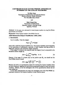
Removing bottlenecks Examining (5), one sees that a natural bound on Var[Yθ ] is obtained by “splitting an edge” in T. Definition 7 (Edge splitting). Let T be an ultrametric tree with edge set E. Let b0 = (x0 , y0 ) be a branch in T (where x0 is closer to the root) and let bi = (y0 , yi ), i = 1, . . . , D, be the outgoing edges at y0 . The operation of splitting branch b0 to obtain a new tree T0 with edge set E 0 is defined as follows: remove b0 , b1 , . . . , bD from T; add D new edges b0i = (x0 , yi ) of length |b0 | + |bi |, i = 1, . . . , D (see Figure 1). We call merging the opposite operation of undoing the above splitting. Note that the number of tips in T and T0 above are the same, and therefore we can use the same estimator Yθ on both of them. Lemma 6 (Splitting an edge). Let T be an ultrametric tree, let b0 be a branch in T, and let T0 be obtained from T by splitting b0 . Then for any nonnegative θ = (θ` )`∈L VarT0 [Yθ ] ≤ VarT [Yθ ]. 18

y1 x0

y1

y2

y0

y2

x0

...

... yD

yD

Figure 1: Edge splitting procedure. Proof. We use the notation of Definition 7. Denote by (θb )b∈E and (θb0 )b∈E 0 the flows associated to θ by (4) on T and T0 respectively. For any branch b, except b0 , b1 , . . . , bD and b01 , . . . , b0D , we have θb = θb0 , as the descendant leaves of b on T and T0 are the same. Think of b0i = (x0 , yi ), i = 1, . . . , D, as being made 00 0 of two consecutive edges b00i = (x0 , yi0 ) and b000 i = (yi , yi ) with |bi | = |b0 | and ). Then, θbi = θb000 + Rb000 |b000 i | = |bi | (and note, for sanity check, that Rb0i = Rb00 i i i , and by (5) and Rbi = Rb000 i VarT [Yθ ] − VarT0 [Yθ ] = Rb0 θb20 −

D X

Rb00i θb200i

i=1

= Rb0

D X i=1

!2 θb00i

− Rb0

D X

θb200i

i=1

≥ 0, where we used that Rb0 = Rb00i and the nonnegativity of the θb00i ’s. Comparing T to a star we then get: Proposition 3 (Lower bound on the variance of µ ˆML ). Let T be an ultrametric tree with n tips and height T . Then   1 − e−2αT −2αT VarT [ˆ µML ] ≥ γ e + . n Proof. Split all edges in T by repeatedly applying Lemma 6 until a star tree with n leaves and height T is obtained. The result then follows from (2). Proceeding in reverse:

19

Proposition 4 (Upper bound on the variance of µ ˆML ). Let T be an ultrametric tree with height T . Recall that πt be the set of points at distance t from the root. Then   1 − e−2α(T −t) −2α(T −t) VarT [ˆ µML ] ≤ inf γ e + . 0≤t≤T |πt | Proof. Let 0 ≤ t ≤ T . For all points x in πt , choose one descendant leaf `x of x and define θ as ( 1 , if ` = `x for some x, |πt | θ` = 0, otherwise. Divide all branches crossing πt into two branches meeting at πt . Then merge all branches above πt (that is, closer to the root) by repeatedly applying Lemma 6. By (5), removing all branches b with θb = 0 does not affect the variance, and from Example 6 with H = 2, D0 = 1, D1 = |πt |, τ0 = t, and τ1 = T − t, we get   2α(T −t) −2αT −2αt 2αt −2α(T −t) 2αt e VarT [ˆ µML ] ≤ γe 1 + (1 − e )e + (1 − e )e |πt |   −2α(T −t) 1−e ≤ γ e−2α(T −t) + . |πt |

The two estimators µ ˆML vs. Y As an application of the previous corollary, we provide an example where µ ˆML performs significantly better than Y . Roughly, the example shows that Y can perform poorly on asymmetric trees. Example 7. Consider a caterpillar sequence (Tk )k , as defined in Example 3, with t2m+1 = m and t2m = 1 for all m, as shown in Figure 2. Let πtk be the time t cutset of Tk and let Tk be the height of Tk . Note that T2m+1 = T2m+2 = m and 2m+1 2m+2 |πm−1 | = |πm−1 | = m. Therefore, by Proposition 4,    1 −2α(m−1) → 0, max VarT2m+1 [ˆ µML ], VarT2m+2 [ˆ µML ] ≤ γ e + m as m → +∞, and hence µ ˆML is consistent. On the other hand, note that Cov[Yi , Yj ] ≥ 0 for all pairs of leaves i, j in Tk . Therefore, " 2m # " m # m X X   1 1 1 X VarT2m Y = Var Y ≥ Var Y = Cov[Y2i , Y2j ] ` 2i 2 2 4m2 4m 4m i=1 i,j=1 `=1 ≥

1 γe−2α 2 −2α m γe = . 4m2 4 20

So, Y is not consistent. Y2n+1 Y5

...

Y3

... n

3 Time

2

Y1 Y2 Y4 Y2n

1 0

Figure 2: Example where the MLE µ ˆ is consistent while Y is not.

3.2

Criterion for consistency of the MLE

In the previous subsection, we gave an example where Y is not consistent for µ, but µ ˆML is. Here we give a general criterion under which µ ˆML is consistent. Theorem 1 (Consistency of µ ˆML ). Let (Tk )k be a sequence of trees satisfying (k) Assumption 1. Let µ ˆML be the corresponding sequence of MLEs of µ given α. Denote by π ˜tk the cutset of Tk at time t away from the leaves and let Tk be the (k) height of Tk . Then (ˆ µML )k is consistent for µ if and only if for all s ∈ (0, +∞) k ˜s = +∞. (10) lim inf π k

Proof. Assume (10) holds. From Proposition 4, for all s,   1 − e−2αs (k) −2αs lim sup VarTk [ˆ µML ] ≤ lim sup γ e + ≤ γe−2αs . k| |˜ π k k s Taking s to +∞ gives consistency. On the other hand, assume by contradiction (k) that (ˆ µML )k is consistent but that k lim inf π ˜s < +∞, k

21

for some s ∈ (0, +∞). Let (kj )j be the corresponding subsequence and L, the k limit above. Divide all branches in Tkj crossing π ˜s j into two branches meeting k k at π ˜s j . Split edges in Tkj above π ˜s j (closer to the root) repeatedly until the tree k above π ˜s j forms a star. Let T0 be the resulting tree, let b01 , . . . , b0D be the branches emanating from the root, where D ≤ L by assumption, and let π ˜ 0 be the cutset at time s from the leaves. For the unit flow θ 0 corresponding to the MLE on T0 , by Lemma 6 and counting only those edges above π ˜ 0 in T0 in (5), we have # " D   X (kj ) −2αTkj −2α(Tkj −s) 2α(Tkj −s) (θb0 0i )2 VarTkj [ˆ µML ] ≥ γe 1+ 1−e e "

2α(Tkj −s)

 e ≥ γe−2αTkj 1 + 1 − e−2α(Tkj −s)

#i=1

D   −2αs   −2αTkj −2α(Tkj −s) e + 1−e ≥ γ e , L 2 , subject to β1 + · · · + βD = 1, is where we used the fact that β12 + · · · + βD minimized at β1 = · · · = βD = 1/D. Since Tkj → +∞ under Assumption 1, (k)

lim sup VarTk [ˆ µML ] ≥ γ k

e−2αs > 0, L

and we get a contradiction. Corollary 1 (Consistency: Nested sequence). Let (Tk )k be a nested sequence satisfying Assumption 1. Then the MLE for µ is consistent on (Tk )k . Proof. Let kj be the subsequence such that Tkj+1 > Tkj for every j and Ti = Tkj for all i = kj + 1, . . . , kj+1 − 1. Then, for all s ∈ (0, +∞), as k goes to +∞ πsk eventually contains all leaves kj such that Tkj ≥ s. Since Tk → +∞ by Assumption 1, the result follows. For nested sequences, it was shown in [16] that Assumption 1 is necessary, as on bounded-height tree sequences the MLE of µ is not consistent. Corollary 2 (Consistency: Growing sequence). Let (Tk )k be a growing sequence satisfying Assumption 1. Then the MLE for µ is consistent on (Tk )k . Proof. Fix s ∈ (0, +∞). For L = 1, 2, . . ., let kL0 be the smallest k such that nk ≥ L and let kL00 be the smallest k > kL0 such that Tk ≥ TkL0 + s. Then, for all k ≥ kL00 , |πsk | ≥ L. Letting L go to +∞ gives the result. 22

More generally, Assumption 1 does not suffice, as the following example shows. Example 8 (Consistency: Counter-example). Using the notation of Example 6, let (T2m )m be a sequence of spherically symmetric trees with H = 2, degrees (2m) (2m) (2m) (2m) D0 = 2, D1 = m, τ0 = m − 1, and τ1 = 1. Although n2m = 2m → +∞ and T2m = m → +∞, that is, Assumption 1, we have by (7)   2α(m−1) 2αm (2m) −2α(m−1) e −2α e −2αm 1 + (1 − e ) + (1 − e ) VarT2m [ˆ µML ] = γe 2 2m −2α e ≥ γ > 0, 2 and the MLE is not consistent. Taking s = 1 in (10) explains why. However, in general, the branching number does provide a simple, sufficient condition. Proposition 5 (Consistency: Branching number condition). Let T = (Tk )k be a tree sequence satisfying Assumption 1 with branching number Λb . Then Λb > 0 suffices for the consistency of the MLE of µ. Note that this condition is independent of α. Proof. By Proposition 2, taking 0 < Λ < min{2α, Λb },   2α (k) e−ΛTk → 0, VarTk [ˆ µML ] ≤ γ 1 + IΛ (2α − Λ) as k → +∞. The condition in Proposition 5 is not necessary, as the following example shows. Example 9 (Caterpillar sequence: Consistency). Using the notation of Example 3, let T = (Tk )k be a caterpillar sequence with tk = ω(log k). The MLE of µ is consistent on T by Corollary 1. However let Λ > 0. For k = 1, 2, . . . X inf e−Λδk (ρ,x) ≤ ke−Λω(log k) → 0, π∈Πk

x∈π g

as k → +∞, where we used that Tk ≥ tk . Therefore Λb = Λ = 0.

23

3.3

Phase transition on the rate of convergence of the MLE

We provided necessary and sufficient conditions for the consistency of the MLE of µ. Moreover we showed that, under Assumption 1, the MLE is consistent for nested and growing sequences. Here we provide bounds on the rate of conver√ gence of the MLE. In particular we give conditions for nk -consistency. We show that the latter undergoes a phase transition, generalizing Example 5. √ Loss of nk -consistency When the upper growth is above 2α, we show that the √ MLE of µ cannot be nk -consistent. If further the branching number is above 2α, we give tight bounds on the convergence rate of the MLE. Roughly we show that, 2α/Λg in the latter case, the variance behaves like nk . Or perhaps a more accurate 2αTk , in the sense way to put it is that the “effective number of samples” neff k is e (k) eff −1 that VarTk [ˆ µML ] = Θ((nk ) ). Theorem 2 (Convergence rate of µ ˆML : Supercritical regime). Let (Tk )k be a g tree sequence. If Λ > 2α, then for all  > 0 there is a subsequence (kj )j along which g (k ) −2α/(Λ −) . (11) VarTkj [ˆ µMLj ] ≥ γnkj √ (k) In particular (ˆ µML )k is not nk -consistent. If, further, 1. Λb > 2α: then
(k) VarTk [ˆ µML ] = Θ e−2αTk . Moreover in terms of nk , for all  > 0, there are constants 0 < C 0 , C < +∞ such that g −2α/(Λ +) −2α/(Λg −) (k) C 0 nk ≤ VarTk [ˆ µML ] ≤ Cnk , (12) and, in addition to (11), (k0 )

−2α/(Λg +)

∃ subsequence (kj0 )j , s.t. VarTk0 [ˆ µMLj ] ≤ γnk0

.

j

j

(13)

2. Λb < 2α: then, for all  > 0, there are constants 0 < C 0 , C < +∞ such that g (k) −(Λb −)/(Λ +) −2α/(Λg −) ≤ VarTk [ˆ µML ] ≤ Cnk C 0 nk , (14) where the lower bound in (14) holds provided Λg > 0, and (k0 )

−(Λb −)/(Λg +)

∃ subsequence (kj0 )j , s.t. VarTk0 [ˆ µMLj ] ≤ γnk0 j

24

j

.

(15)

g

Proof. Assume Λ > 2α. As remarked after Definition 4, for all  > 0, eventually
g exp ((Λg − )Tk ) ≤ nk ≤ exp (Λ + )Tk , (16) that is, −2α/(Λg −)

nk

g

−2α/(Λ +)

≤ e−2αTk ≤ nk

.

(17)

Moreover for all  > 0 there are subsequences (kj )j and (kj0 )j such that  
g nkj ≥ exp (Λ − )Tkj and nkj0 ≤ exp (Λg + )Tkj0 .

(18)

By Proposition 3, (k) VarTk [ˆ µML ]

 ≥γ e

−2αTk

 1 − e−2αTk + ≥ γe−2αTk . nk

(19)

√ (k) Then (11) follows from (18) and (19). Hence (ˆ µML )k is not nk -consistent by Lemma 3. Assume Λb > 2α. Let 2α < Λ < Λb . By Proposition 2   2α (k) e−2αTk . (20) VarTk [ˆ µML ] ≤ γ 1 + IΛ (Λ − 2α) g

Note that Λ ≥ Λg ≥ Λb > 2α and hence, by (19) and (20),
(k) VarTk [ˆ µML ] = Θ e−2αTk . Combining the last equation with (16) gives the result in terms of nk . Assume instead that Λb < 2α. Let Λ < Λb . By Proposition 2   2α (k) VarTk [ˆ µML ] ≤ γ 1 + e−ΛTk . IΛ (2α − Λ)

(21)

The rest of the argument is similar to the previous case. The following example shows that, when Λb < 2α, our upper bound on the variance may not be achieved, but cannot be improved in general.

25

Example 10 (Two-level tree). Let (Tk )k be a sequence of spherically symmetric (k) (0) (k) (k) trees, as defined in Example 6, with H = 2, D0 = eΛ0 τ0 D1 = eΛ1 τ1 , for some Λ0 < Λ1 and

(k) τ0 (k) (k) τ0 +τ1

(k)

VarTk [ˆ µML ] = γe

= σ, with 0 < σ < 1. Then, by (7),

(k) (k) −2α(τ0 +τ1 )

(k)

" 1+

X

(k) −2ατh

(1 − e

)

(k)

(k)

+τ1 )

(k)

(k)

+ (1 − e−2ατ0 )e−(Λ0 τ0 (k)

Dh0 (k)

+2ατ1 )

(k)

+(1 − e−2ατ1 )e−(Λ0 τ0

#

(k)

h0 =0

h=0,1

= γ[e−2α(τ0

h Y e2ατh0

(k)

+Λ1 τ1 )

].

(22)

Note that (k)

(k)

log nk Λ0 τ0 + Λ1 τ1 = (k) (k) Tk τ0 + τ1

= Λ0 σ + Λ1 (1 − σ) = Λg .

To compute the branching number, it suffices to consider cutsets with m0 middle (k) (k) vertices and the D1 (D0 − m0 ) tips below the rest of the middle vertices. Then ( (k) (k) (k) (k) X D0 e−Λτ0 , if D1 > eΛτ1 −Λδk (ρ,x) Jk ≡ inf e = π∈Πk nk e−ΛTk , otherwise. x∈π Hence if Λ ≥ Λ1 > Λg we are in the second case and nk e−ΛTk = e−(Λ−Λ

g )T k

→ 0,

as k → +∞. If Λ < Λ1 we are in the first case and (k)

(k)

(k)

D0 e−Λτ0 = e−(Λ−Λ0 )τ0 , so that Λb = Λ0 . If Λb = Λ0 ≥ 2α, the dominant term in the variance is (k) (k) −2α/Λg γe−2α(τ0 +τ1 ) = γnk , as predicted by Theorem 2. If instead Λb = Λ0 < 2α, there are two cases. If Λ1 ≤ 2α, the dominant term in the variance is (k)

γe−(Λ0 τ0 and we have variance is

√

= γe−Λ

gT k

= γn−1 k ,

nk -consistency. If instead Λ1 > 2α, the dominant term in the

(k)

γe−(Λ0 τ0

(k)

+Λ1 τ1 )

(k)

+2ατ1 )

= γe−(Λ

b σ+2α(1−σ))T k

26

−(2α/Λg )(1−σ)−(Λb /Λg )σ

= γnk

.

Therefore, depending on the value of σ, we can get the full range of exponent values between (12) and (14). Note also that by taking Λ1 large enough and √ σ close enough to 1 it is possible to have Λg < 2α, yet not nk -consistency. (Below, we will consider imposing the extra condition Λb = Λg . Then we must have Λ0 = Λ1 and this case cannot arise.) √ Conditions for nk -consistency The previous example also shows that when g the upper growth is below 2α, the picture is somewhat murky. (In fact if Λ = 0 we may not have consistency, as Example 8 shows.) The issue in Example 10 is the inhomogeneous growth rate. However, under extra regularity conditions, √ nk -consistency can be established. We give examples in the next section. (k)

Theorem 3 (Convergence rate of µ ˆML : Subcritical regime). Let (Tk )k be a tree g sequence with Λ < 2α. Then
(k) VarTk [ˆ µML ] = Ω n−1 . k Further if: g

1. [Equality of growth and branching number] Λb = Λ > 0 then for all  > 0   (k) −(1−) VarTk [ˆ µML ] = O nk . 2. [Bounded uniform growth] Λug < 2α then
(k) VarTk [ˆ µML ] = O n−1 . k Proof. One direction follows immediately from Proposition 3 which implies (k)

VarTk [ˆ µML ] ≥ γ

1 − e−2αTk = Ω(n−1 k ). nk

We prove the other direction separately in each case. g Assume first that 0 < Λb = Λ < 2α. For  > 0 (small), choose Λ such that g

g

Λ −  < Λ < Λ = Λb < 2α. By Proposition 2, eventually (k) VarTk [ˆ µML ]

  2α ≤ γ 1+ e−ΛTk IΛ (2α − Λ)   g g 2α −(Λ −)/(Λ +) ≤ γ 1+ nk . IΛ (2α − Λ) 27

Assume instead that Λug < 2α. We show that Y (and hence the MLE by √ Proposition 1) achieves nk -consistency in this case. Let θ be the corresponding flow on Tk . By Lemma 5, letting Λug < Λ < 2α, for k large enough     Z Tk X  nk (x) 2  ds e2αs  VarTk [Y ] = γe−2αTk 1 + 2α n k 0 x∈πsk     Z Tk X  nk (x)  eΛ[(Tk −s)+M ]  ds e2αs  ≤ γe−2αTk 1 + 2α n n k k 0 x∈πsk   2α ΛTk (2α−Λ)Tk −2αTk ΛM e (e − 1) ≤ γe 1+e nk (2α − Λ)   2α −2αTk ΛM −(2α−Λ)Tk = γ e +e (1 − e ) . nk (2α − Λ) The result follows from the fact that eΛ[Tk +M ] ≥ nk .

3.4

Special cases

Bounded branch lengths. We first consider binary, ultrametric species trees with bounded edge lengths, where binary means the out-degree of every vertex is 2 except for the leaves. Corollary 3 (Special case: Bounded edge lengths). Let (Tk )k be a sequence of binary, ultrametric trees with edge sets Ek and f = inf |b|,

g = sup |b|,

k,b∈Ek

k,b∈Ek

satisfying Assumption 1. Then the following hold. (k)

1. If f > 0, then µ ˆML is consistent. (k)

√ nk -consistent.

2. If f >

log 2 , 2α

then µ ˆML is

3. If g
0, for a point x in Tk nk (x) ≤ 2Tk (x)/f , so that

k nk π ˜s ≥ s/f → +∞. 2 log 2 2α(1−)

If further f ≥

Tk (x)/f

nk (x) ≤ 2

for some  > 0,  ≤ exp

(log 2)Tk (x) f

 ≤ exp (2α(1 − )Tk (x))

so that Λug < 2α, and the second result follows from Theorem 3. log 2 If instead g ≤ 2α(1+) for some  > 0, Tk /g

nk ≥ 2

 ≥ exp

(log 2)Tk g

so that

 ≥ exp (2α(1 + )Tk )

g

Λ > 2α, and the second result follows from Theorem 2. Yule model We also specialize the results to the Yule model. Corollary 4 (Special case: Yule model). Let (Tk )k be a Yule sequence, as defined in Example 4, with rate 0 < λ < +∞. Then, with probability 1 (on the generation of T0 ), (k)

1. (ˆ µML )k is consistent. (k)

2. If λ < 2α, (ˆ µML )k is

√

nk -consistent.

(k)

3. If λ > 2α, (ˆ µML )k is not 0 C , C < +∞ such that C 0 n−2αλ k

√

−1 −

nk -consistent and for all  > 0 there is 0 < (k)

−1 +

≤ VarTk [ˆ µML ] ≤ Cn−2αλ k

29

.

g

Proof. By Theorems 1, 2, and 3, it suffices to prove that Λb = Λ = λ with probability 1. A Galton-Watson (GW) branching process is a discrete-time non-negative integer-valued population process defined as follows: at each time step, each individual in the population has an independent number of offsprings, according to a distribution F , that form the population at the next time. In [20], it is shown that a GW tree where F has mean m has branching number and upper growth equal to log m. To compute the branching number of an infinite Yule tree T0 , we use a comparison to a GW tree. Fix  > 0. Let F be the distribution of the number of lineages in T0 at time . By standard branching process results [4], m = eλ . By the memoryless property of the exponential, the number of lineages |πN  | in the Yule tree at time N  is identically distributed to the population size ZN of a GW tree with offspring distribution F at time N . Then log Zds/e ds/e log Zds/e log |πs | ≤ = · , s s s ds/e which implies that 1 · log eλ = λ.  Similarly, let π be a cutset in T0 and let π be the cutset obtained by rounding up the points in π to the next -multiple closer to the root (removing duplicates). Let δGW (v) be the distance from the root to vertex v in the GW tree. Then X X X e−Λ(δGW (y)+1) = e−Λ e−(Λ)δGW (y) > 0 e−Λδ0 (ρ,x) ≥ g

Λ ≤

x∈π

y∈π

y∈π

whenever Λ < log eλ , so that Λb ≥ λ.

3.5

Sensitivity to estimate of α

So far in this section, we considered the MLE of µ given α. Here we look at the sensitivity of the MLE to estimation errors on α. In the next section, we provide √ conditions under which a nk -consistent estimator of α exists. In particular, these conditions are unrelated to the growth or height of the species tree, and apply to 30

the two special cases above. Moreover the estimator of α we derive does not require the knowledge of µ. √ dT ˆ k of α. Let Var Hence suppose that we have a nk -consistent estimator α k denote the variance under the parameter α = α ˆ k (with µ and γ unchanged) and let ˆ k be the corresponding weights of the MLE of µ, that is, the choice of weights θ d T [Yθ ]. assuming that α = α ˆ k and minimizing Var k For all k and under the true α, Yθˆ k is an unbiased estimator of µ. Moreover, because α ˆ k = α + o(1) and so on, the bounds in Theorems 2 and 3 apply to d VarTk [Yθˆ k ] as well (for k large enough). The quantity of interest is VarTk [Yθˆ k ]. By Lemma 4, VarTk [Yθˆ k ] = γe−2αTk + γ

X

(1 − e−2α|b| )e2α(δk (ρ,b)−Tk ) (θˆk )2b

b∈Ek

"

#

= (1 +

−1/2 O(Tk nk ))

= (1 +

−1/2 d O(Tk nk ))Var ˆ k ], Tk [Yθ

γe−2αˆ k Tk + γ

X

(1 − e−2αˆ k |b| )e2αˆ k (δk (ρ,b)−Tk ) (θˆk )2b

b∈Ek

−1/2

provided Tk nk = o(1). Hence, for instance if Λg > 0, Tk = O(log nk ) and we get that VarTk [Yθˆ k ] satisfies the bounds in Theorems 2 and 3.

4

Convergence rate of a new estimator for α and γ

In this section, we provide a novel estimator for (α, γ). Under natural assumptions √ on the species tree, we show that this estimator is nk -consistent. Moreover this estimator does not require the knowledge of µ. Interestingly, in contrast to √ what we showed for µ, the conditions for nk -consistency in this case do not involve the growth —or even the height— of the species tree. This is in line with the results in [16], who found that µ requires an unbounded tree height to be microergodic, whereas α and γ do not. Note, however, that the MLE of α and γ are not simple linear estimators, which makes them harder to study here. In particular, unlike in the case of µ, we do not provide lower bounds on their rate of convergence. We illustrate our estimator in two special cases.

31

4.1

Contrast-based estimator

We first describe the estimator. The analysis of its convergence rate is performed in Section 4.2. Contrasts Our estimator relies on an appropriately chosen set of contrasts, that is, differences between pairs of leaf states (see e.g. [12]). More specifically, we choose contrasts associated with internal nodes, as follows. Let T be an ultrametric species tree with leaves L and internal vertices I . For two leaves ` and `0 , we let ` ∧ `0 be their most recent common ancestor. Assume that all internal vertices of T have out-degree at least 2. Let i ∈ I be an internal vertex of T, and let `i1 6= `i2 be two leaves such that `i1 ∧ `i2 = i. Let Pi be the path connecting `i1 and `i2 . We define the corresponding contrast Ci = Y`i1 − Y`i2 . Let T (i) be the height of i from the leaves. We say that T (i) is the height of Ci . Lemma 7 (Contrasts: Distribution [16]). Let i1 , . . . , im be a collection of internal nodes of T. Let Ci1 , . . . , Cim be an arbitrary set of associated contrasts. Assume that the corresponding paths Pi1 , . . . , Pim are pairwise non-intersecting, that is, none of the pairs of paths share a vertex. Then Ci1 , . . . , Cim are mutually independent, multivariate normal with Ci ∼ N (0, 2γ(1 − e−2αT (i) )). Proof. Indeed, expanding the covariance, we get for j 6= j 0 −αd

γ −1 Cov[Cj , Cj 0 ] = e

j j0 `1 `1

−e

−αd

j j0 `1 `2

−αd

−e

j j0 `2 `1

+e

−αd

j j0 `2 `2

= 0,

0

since, by assumption, `jι ∧ `jι0 is the same vertex for all ι, ι0 = 1, 2. The following lemma will be useful in identifying an appropriate collection of contrasts. Lemma 8 (Contrasts: A large collection [16]). Let T be an ultrametric tree and let I(a,b) be the set of internal nodes of T whose height from the leaves lies in (a, b). For every a < b, we can select a set of independent contrasts C , associated with internal nodes in I (a, b), such that |C | ≥ n(a, b)/2, where n(a, b) = |I (a, b)|. In particular, the heights of the contrasts in C lie in (a, b) and their corresponding paths are pairwise non-intersecting.

32

Proof. Start with the lowest vertex i in I(a,b) and choose a pair of vertices `i1 and `i2 such that `i1 ∧ `i2 = i. Remove i and its descendants as well as the edge immediately above i (and fuse consecutive edges separated by degree-2 vertices). As a result, the number of internal vertices in (a, b) decreases by at most 2. Repeat until no vertex is left in I(a,b) . The estimator For a sequence of trees T = (Tk )k , let Lk be the leaf set of Tk ; Ik , the set of its internal vertices; nk = |Lk | and nk (a, b) = |Ik (a, b)|; and Tk (i), the height of i, for each i ∈ Ik . The idea behind our estimator is to set up a system of equations that characterize α and γ uniquely. Our construction relies on the following condition. We illustrate this condition on two special cases below. Assumption 2 (Linear-sized bands). Assume that there are constants 0 < β < 1 and 0 < c1 < c01 < c2 < c02 < ∞ such that nk (cι , c0ι ) ≥ βnk , ι = 1, 2, for all k large enough. We set up our equations as follows. Let mk = bβnk /2c. Under Assumption 2, by Lemma 8, for each k we can choose two collections of independent con0 k mk k trasts (Cikr )m r=1 and (Cjr )r=1 with corresponding heights Tk (ir ) ∈ (c1 , c1 ) and Tk (jr ) ∈ (c2 , c02 ) for every r = 1, 2, . . . , mk . (Note that the two collections are not independent.) For r = 1, . . . , m, let mk 1 X (k) (Cir )2 , a ˆk = mk r=1

mk X (k) ˆbk = 1 (Cjr )2 , mk r=1

and note that ak ≡ IE[ˆ ak ] = 2γ bk

h i ≡ IE ˆbk = 2γ

mk 1 X 1− e−2αTk (ir ) mk r=1

!

mk 1 X 1− e−2αTk (jr ) mk r=1

≡ 2γh1k (α), ! ≡ 2γh2k (α).

Notice that, under Assumption 2, ak ∈ [2γ(1 − e−2αc2 ), 2γ(1 − e−2αc1 )] ≡ [aα , a ¯α ] −2αc4 −2αc3 ¯ and bk ∈ [2γ(1 − e ), 2γ(1 − e )] ≡ [bα , bα ]. As shown below, Hk (α) =

ak h1 (α) = k2 bk hk (α) 33

is invertible in α on (0, +∞). Hence a natural estimator of (α, γ) is obtained by setting   a ˆk −1 , (23) α ˆ k = Hk ˆbk a ˆk . (24) γˆk = 1 αk ) 2hk (ˆ We will show in the proof of invertibility below that Hk is actually strictly increasing, and therefore relatively straightforward to invert numerically. It remains to prove invertibility. Lemma 9 (Invertibility of the system). Under Assumption 2, Hk (α) is strictly positive, differentiable, and invertible on (0, +∞). Proof. We have that Pmk Pmk −2αTk (jr ) 2Tk (ir )e−2αTk (ir ) r=1 2Tk (jr )e r=1 Pmk P − mk −2αTk (ir ) ) −2αTk (jr ) ) r=1 (1 − e r=1 (1 − e PP mk −2αTk (ir ) (1 − e−2αTk (jr0 ) ) r,r0 =1 2Tk (ir )e Pmk = Pmk −2αTk (jr ) ) −2αTk (ir ) ) r=1 (1 − e r=1 (1 − e P Pmk −2αTk (jr0 ) (1 − e−2αTk (ir ) ) r,r0 =1 2Tk (jr0 )e Pmk (25) − Pmk −2αTk (jr ) ) −2αTk (ir ) ) r=1 (1 − e r=1 (1 − e

∂ log Hk (α) = ∂α

Note that the function is

e−x (1−x−e−x ) (1−e−x )2

xe−x 1−e−x

is strictly decreasing on (0, ∞) because its derivative

< 0 on (0, +∞). Therefore 0

2c01 e−2αc1 2c2 e−2αc2 2Tk (ir )e−2αTk (ir ) 2Tk (jr0 )e−2αTk (jr0 ) ≥ > , ≥ 0 1 − e−2αTk (ir ) 1 − e−2αc2 1 − e−2αTk (jr0 ) 1 − e−2αc1 that is, 2Tk (ir )e−2αTk (ir ) (1 − e−2αTk (jr0 ) ) −2Tk (jr0 )e−2αTk (jr0 ) (1 − e−2αTk (ir ) ) > 0,

(26)

for every r, r0 , so that each (r, r0 )-term in (25) is strictly positive. Hence, we can deduce that ∂ log Hk (α)/∂α > 0, that is, log Hk (and hence Hk itself) is strictly increasing on (0, +∞) and continuous, and therefore invertible. Note that we cannot use the law of large numbers to derive consistency (despite the independence of the contrasts) because ak /bk is a bounded, but not necessarily convergent, sequence and Hk−1 is continuous, but depends on k. Instead √ we argue directly about nk -consistency below. 34

4.2

Rate of convergence √

nk -consistency of our estimator for (α, γ). √ Theorem 4 (Estimating α and γ: nk -consistency). Let T = (Tk )k be a sequence of ultrametric trees satisfying Assumptions 1 and 2 and let (ˆ αk , γˆk )k −1/2 be the estimator defined in (23) and (24). Then |ˆ αk − α| = Op (nk ) and −1/2 |ˆ γk − γ| = Op (nk ). Our main result in this section is the

Proof. Note that IE[ˆ ak ] = ak and Var[ˆ ak ] =

mk 8γ 2 8γ 2 X −1 −2αTk (ir ) 2 ) ≤ (1 − e (1 − e−2αc1 )2 = O(m−1 k ) = O(nk ), 2 mk r=1 mk

where we used that ([2γ(1 − e−2αTk (ir ) )]−1/2 Cikr )2 is χ21 -distributed and, therefore, −1/2 has variance 2. Hence, by Lemma 2, |ˆ ak − ak | = Op (nk ). Similarly, |ˆbk − bk | = −1/2 −1/2 Op (nk ). Our claim that |ˆ αk −αk | = Op (nk ) then follows from the following straightforward lemmas. Lemma 10. Let x, y be two positive numbers such that 0 < x∗ ≤ x ≤ x∗ < ∞ and 0 < y∗ ≤ y ≤ y ∗ < ∞. Assume that |x − x0 | ≤  and |y − y 0 | ≤  with  < y∗ /2. Then 0 ∗ ∗ x x − < 4(x + y ) . y0 y y∗2 Proof. We have 0 0 0 ∗ 0 ∗ 0 x − x = y(x − x) + x(y − y ) ≤ y |x − x| + x |y − y | . y0 y yy 0 y∗ (y∗ /2) y∗ (y∗ /2)

Lemma 11. If 0 < z∗ ≤ z ≤ z ∗ < ∞, |z 0 − z| ≤  and  < z∗ /2, then there is a constant ∆(z∗ , z ∗ ) depending on c1 , c01 , c2 , c02 such that for all k sup |(Hk−1 )0 (tz 0 + (1 − t)z)| ≤ ∆(z∗ , z ∗ ).

t∈[0,1]

35

Proof. We use the proof of Lemma 9. Let ζα = ζα (c1 , c01 , c2 , c02 ) > 0 be the smallest possible difference in (26) for a fixed α. Let α∗ , α∗ be defined as a ¯α 3 ∗ aα∗ 1 z∗ = ∗ , z =¯ . 2 bα ∗ 2 bα ∗  
Then [α∗ , α∗ ] ⊇ Hk−1 12 z∗ , 32 z ∗ for all k. Note that sup |(Hk−1 )0 (tz 0 + (1 − t)z)| ≤ sup (Hk−1 )0 (z) t∈[0,1] z∈[ 12 z∗ , 23 z ∗ ]  −1 ∂Hk −1 = sup (Hk (z)) ∂α z∈[ 21 z∗ , 23 z ∗ ]   −1 ∂ log Hk −1 (Hk (z)) Hk = sup ∂α z∈[ 21 z∗ , 23 z ∗ ] 0

0

bα (1 − e−2αc1 )(1 − e−2αc2 ) · ≤ sup ¯α ζα α∈[α∗ ,α∗ ] a ≡ ∆(z∗ , z ∗ ).

i Theorem 4. Fix δ > 0 (small) and pick Mδ such that h We finish the proof of −1/2 < δ/2 and similarly for ˆbk . Then, by Lemma 10 and IP |ˆ ak − ak | ≥ Mδ nk Assumption 1, for k large enough   a ˆk ak 4(¯ aα + ¯bα ) −1/2 IP − ≥ Mδ nk ˆbk bk b2α   ¯bα ) a 4(¯ ˆ a + a k k α −1/2 −1/2 −1/2 ≤ IP − ≥ Mδ nk , |ˆ ak − ak | ≤ Mδ nk , |ˆbk − bk | ≤ Mδ nk ˆbk bk b2α h i h i −1/2 −1/2 +IP |ˆ ak − ak | ≥ Mδ nk + IP |ˆbk − bk | ≥ Mδ nk ≤0+ so that

δ δ + = δ, 2 2 a ˆk − ak = Op (n−1/2 ). k ˆb bk k

36

Secondly, using Rolle’s theorem, we have   −1 0 a a ˆ ˆ a a k k k k . − . |ˆ αk − α| ≤ sup (Hk ) t + (1 − t) ˆbk bk ˆbk bk t∈[0,1] Let Mδ be such that   a ˆ a k k −1/2 IP − ≥ Mδ nk < δ. ˆbk bk Fix 0 > 0 and let

a 0 a ¯α+0 . z∗ = z∗ = ¯α− , bα+0 bα−0 Then, by Lemma 11, letting ( )   −1 0 a a ˆ a ˆ a k k k m −1/2 . ≥ ∆−1 (z∗ , z ∗ )Mδ n Hk = sup (Hk ) t + (1 − t) , − k ˆ ˆ b b k m bk bm t∈[0,1]

we have for k large enough i h −1/2 −1 ∗ IP |ˆ αk − α| ≥ ∆ (z∗ , z )Mδ nk ≤ IP[Hk ]     a a ˆk ak ˆk ak −1/2 −1/2 ≤ IP Hk , − < Mδ nk + IP − ≥ Mδ nk ˆbk ˆbk bk bk ≤ 0 + δ = δ. That implies −1/2

|ˆ αk − α| = Op (nk

).

The argument for γˆk is similar. To deal with the denominator, note that h i −1/2 IP 2h1k (ˆ αk ) − 2h1k (α) ≥ Mδ nk " # mk 1 X
−1/2 ≤ IP 2 e−2αˆ k Tk (ir ) − e−2αTk (ir ) ≥ Mδ nk mk r=1 " # mk −2αˆ T (i ) 1 X −1/2 e k k r − e−2αTk (ir ) ≥ Mδ n ≤ IP 2 k mk r=1 " # mk 1 X −1/2 ≤ IP 2 2Tk (ir ) |ˆ αk − α| ≥ Mδ nk mk r=1 h i −1/2 ≤ IP 4c1 |ˆ αk − α| ≥ Mδ nk , 37

where we used that |e−x − e−y | ≤ |x − y| for x, y ≥ 0. Then use Lemma 10 as above. Remark 2. The previous result can be further generalized to sublinear-sized collections of contrasts whose height grows with k (with a different rate of convergence). We leave out the details.

4.3

Special cases

We show that Assumption 2 is satisfied in two natural settings. Bounded edge lengths edge sets Ek and

Let (Tk )k be a sequence of binary, ultrametric trees with

f = inf |b|,

g = sup |b|,

k,b∈Ek

k,b∈Ek

satisfying Assumption 1. Corollary 5 (Special case: Bounded edge lengths). If 0 < f ≤ g < +∞ then As−1/2 −1/2 sumption 2 is satisfied, and hence |ˆ αk −α| = Op (nk ) and |ˆ γk −γ| = Op (nk ). Proof. By Theorem 4 it suffices to show that Assumption 2 is satisfied. We claim that nk (f, g) ≥ nk /2 (27) and nk (2g, 3g) ≥ nk /22g/f so that we can take c1 = f , c01 = g, c2 = 2g, and c02 = 3g. Indeed, looking backwards in time, by the definition of f and g the nk lineages originating from the leaves cannot coalesce in the (0, f ) time interval, but must coalesce at least once in the (f, g) time interval. Then (27) follows from our assumption that Tk is binary. Similarly the largest possible number of descendant leaves of a point at height 2g is 22g/f . Hence the number of lineages at time 2g is at least nk /22g/f and all such lineages must coalesce at least once in the next g-length time interval, looking backwards.

38

Yule model We also apply the results to the Yule model. For simplicity, we take a special sequence of times (although this assumption is not crucial). Let T0 be an infinite Yule tree with rate 0 < λ < +∞. For k ≥ 1, let tk be the first time at which T0 has k + 1 lineages. Then nk = k for all k and tk → +∞ so that Assumption 1 is satisfied. Corollary 6 (Special case: Yule model). Let (Tk )k be a Yule sequence as above. −1/2 Then Assumption 2 is satisfied asymptotically, and hence |ˆ αk − α| = Op (nk ) −1/2 and |ˆ γk − γ| = Op (nk ). Remark 3. Note that, unlike the case of Corollary 4, we do not prove that the result holds with probability 1 on the choice of T0 . That is, the convergence in probability above involves stochasticity over both T0 and the overlaid OU process. Proof. Let τi = ti − ti−1 be the amount of time during which T0 has i lineages (with t0 = 0). Then (τi )i are P independent exponential random variables with j parameters (1/(iλ))i . Let Ti = jr=i+1 τr . Note that j j X X  j 1 −1 , IE Ti = IE[τr ] ≡ λ r r=i+1 r=i+1

with  log

j i+1



Z

j

= i+1

  Z j j X 1 1 1 j dx ≤ ≤ dx ≤ log . x r i i x r=i+1

Similarly, Var[Tij ] =

j X

Var[τr ] = λ−2

r=i+1

with

j X 1 , 2 r r=i+1

(28)

Z +∞ j X 1 1 1 ≤ dx = . 2 2 r x i i r=i+1

By Chebyshev’s inequality, for all 0 < σ < 1,  k  k   IP |Tbσkc − IE Tbσkc | ≥  = O(k −1 ), where we used (28). Let 0 < σ20 < σ2 < σ10 < σ1 < 1. From the previous equation, we get for ι = 1, 2     k k −1 IP Tbσι kc ≤ λ log −  = O(k −1 ), bσι kc + 1 39

and

 IP

k Tbσ 0 ι kc

−1

≥λ

 log

k bσι0 kc







 +  = O(k −1 ).

Take aι = λ

−1

 log

1 σι

 ,

a0ι

=λ

−1

log

1 σι0

and  < a1 ∧

1 [a2 − a01 ] . 2

Then Assumption 2 is satisfied asymptotically with cι = aι − ,

c0ι = a0ι +  and β = [σ1 − σ10 ] ∧ [σ2 − σ20 ],

because then h i k k 0 k k 0 −1 IP c1 < Tbσ < T < c < c < T < T < c 0 0 2 1 bσ2 kc 2 ≥ 1 − O(k ). bσ1 kc bσ2 kc 1 kc

References [1] Radosław Adamczak and Piotr Miło´s. CLT for Ornstein-Uhlenbeck branching particle system. arXiv preprint arXiv:1111.4559, 2011. [2] Radosław Adamczak and Piotr Miło´s. U-Statistics of Ornstein-Uhlenbeck branching particle system. Journal of Theoretical Probability, pages 1–41, 2011. [3] T. W. Anderson. An introduction to multivariate statistical analysis. Wiley, Chichester, 2nd edition, 1984. [4] K.B. Athreya and P. Ney. Branching Processes. Dover Books on Mathematics Series. Dover Publications, 2004. [5] Krzysztof Bartoszek, Jason Pienaar, Petter Mostad, Staffan Andersson, and Thomas F. Hansen. A phylogenetic comparative method for studying multivariate adaptation. Journal of Theoretical Biology, 314:204–215, 2012. [6] Krzysztof Bartoszek and Serik Sagitov. Phylogenetic confidence intervals for the optimal trait value. arXiv preprint arXiv:1207.6488, 2012.

40

[7] David Brawand, Magali Soumillon, Anamaria Necsulea, Philippe Julien, Gabor Csardi, Patrick Harrigan, Manuela Weier, Angelica Liechti, Ayinuer Aximu-Petri, Martin Kircher, Frank W. Albert, Ulrich Zeller, Philipp Khaitovich, Frank Grutzner, Sven Bergmann, Rasmus Nielsen, Svante P¨aa¨ bo, and Henrik Kaessmann. The evolution of gene expression levels in mammalian organs. Nature, 478(7369):343–348, 10/20 2011. [8] Marguerite A Butler and Aaron A King. Phylogenetic comparative analysis: a modeling approach for adaptive evolution. The American Naturalist, 164(6):683–695, 2004. [9] Natalie Cooper and Andy Purvis. Body size evolution in mammals: complexity in tempo and mode. The American Naturalist, 175(6):727–738, 2010. [10] Forrest W Crawford and Marc A Suchard. Diversity, disparity, and evolutionary rate estimation for unresolved Yule trees. Systematic Biology, 62(3):439–455, 2013. [11] W. S. Evans, C. Kenyon, Y. Peres, and L. J. Schulman. Broadcasting on trees and the Ising model. Ann. Appl. Probab., 10(2):410–433, 2000. [12] J. Felsenstein. Inferring Phylogenies. Sinauer Associates, 2004. [13] Joseph Felsenstein. Phylogenies and the comparative method. American Naturalist, 125(1):1–15, 1985. [14] Thomas F Hansen. Stabilizing selection and the comparative analysis of adaptation. Evolution, 51(5):1341–1351, 1997. [15] Luke J. Harmon, Jonathan B. Losos, T. Jonathan Davies, Rosemary G. Gillespie, John L. Gittleman, W. Bryan Jennings, Kenneth H. Kozak, Mark A. McPeek, Franck Moreno-Roark, Thomas J. Near, Andy Purvis, Robert E. Ricklefs, Dolph Schluter, James A. Schulte II, Ole Seehausen, Brian L. Sidlauskas, Omar Torres-Carvajal, Jason T. Weir, and Arne . Mooers. Early bursts of body size and shape evolution are rare in comparative data. Evolution, 64(8):2385–2396, 2010. [16] Lam Si Tung Ho and C´ecile An´e. Asymptotic theory with hierarchical autocorrelation: Ornstein-Uhlenbeck tree models. Annals of Statistics, 41:957– 981, 2013. 41

[17] E.L. Lawler. Combinatorial Optimization: Networks and Matroids. Holt, Rinehart and Winston, 1976. [18] E. Mossel and M. Steel. Majority rule has transition ratio 4 on yule trees under a 2-state symmetric model. Submitted, 2014. [19] Elchanan Mossel, S´ebastien Roch, and Allan Sly. Robust estimation of latent tree graphical models: Inferring hidden states with inexact parameters. IEEE transactions on information theory, 59(7):4357–4373, 2013. [20] Yuval Peres. Probability on trees: An introductory climb. In Pierre Bernard, editor, Lectures on Probability Theory and Statistics, volume 1717 of Lecture Notes in Mathematics, pages 193–280. Springer Berlin Heidelberg, 1999. [21] Rori V Rohlfs, Patrick Harrigan, and Rasmus Nielsen. Modeling gene expression evolution with an extended Ornstein-Uhlenbeck process accounting for within-species variation. Molecular Biology and Evolution, 31(1):201– 211, 2014. [22] C. Semple and A. Steel. Phylogenetics. Oxford lecture series in mathematics and its applications. Oxford University Press, 2003. [23] G Udny Yule. A mathematical theory of evolution, based on the conclusions of Dr. JC Willis, FRS. Philosophical Transactions of the Royal Society of London. Series B, 213:21–87, 1925.

42