PHASE TRANSITIONS AND SHARP-INTERFACE

PHASE TRANSITIONS AND SHARP-INTERFACE LIMITS FOR THE 1D-ELASTICITY SYSTEM WITH NON-LOCAL ENERGY CHRISTIAN ROHDE∗ Abstract. The one-dimensional system of elasticity with a non-monotone or convex-concave stress-strain relation provides a model to describe the longitudinal dynamics of solid-solid phase transitions in a bar. If dissipative effects are neglected it takes the form of a system of first-order nonlinear conservation laws and dynamical phase boundaries appear as shock wave solutions. In the physically most relevant cases these shocks are of the non-classical undercompressive type and therefore entropy solutions of the associated Cauchy problem are not uniquely determined. Important dissipative effects that lead to unique regular solutions are viscosity and capillarity where the latter effect is usually modelled by at least third-order spatial derivatives. Differently from these models we consider a novel type of non-local regularization that models both effects but avoids high-order derivatives. We suggest a particular scaling for the dissipative terms and conjecture that with this scaling the regular solutions single out unique physically relevant weak solutions of the first-order conservation law in the limit of vanishing dissipation parameter. We verify the conjecture first by proving that the non-local system admits special solutions of traveling-wave type that correspond to dynamical phase boundaries. Moreover it is proven that regular solutions of a general Cauchy problem converge to weak solutions of the system of first-order conservation laws. The proof is achieved by the method of compensated compactness. Key words. Non-local energy, viscosity-capillarity, sharp interface limit, undercompressive shock waves.

1. Introduction. We consider the Cauchy problem for the one-dimensional system of elasticity which is given by wt

−

vx

=

0,

vt

−

σ(w)x

=

0,

(1.1)

in R × (0, T ), T > 0, and w(., 0) = w0 ,

v(., 0) = v0 ,

(1.2)

in R. Here the strain w : R × (0, T ) → (−1, ∞) and the velocity v : R × (0, T ) → R are the two unknowns depending on x ∈ R and time t ≥ 0. The given function σ : (−1, ∞) → R is the stressstrain relation and w0 : R → (−1, ∞), v0 : R → R are the initial functions. The system (1.1) governs the longitudinal dynamics of an elastic bar of infinite length at constant temperature. We are interested in materials that occur in different phases and undergo dynamical phase transitions. More specifically we consider the two following choices for σ which describe twophase materials: (a)

σ is a monotone increasing function except in a bounded interval,

(b)

σ is a monotone increasing function but has concave-convex shape.

Examples for materials for which choice (a) applies are shape-memory alloys (see e.g. [31, 43]). The two distinct intervals of strain state for which σ is monotone increasing determine the two different phases. An example for which (b) holds are rubber-like materials (see e.g. [32]). In this case the two distinct intervals of strain states for which either σ convex or σ concave holds determine the two different phases. Formally the system (1.1) with choice (a) or (b) is a nonlinear conservation law. As such standard weak solutions of (1.1) are shock waves connecting two end states. In particular dynamical phase transitions ∗ Albert-Ludwigs-Universit¨ at Freiburg, Institut f¨ ur Mathematik, Hermann-Herder Str. 10, D-79104 Freiburg, Germany ([email protected]).

1

2

C. ROHDE

can be constructed in a natural way as shock waves with strain components of the end states in two different phases. However, if they are of the physically relevant subsonic type, then they do not belong to the class of classical Laxian waves like e.g. hydrodynamical shock waves for Euler’s equations with a perfect gas. Rather these waves are called non-classical undercompressive waves ([34] or [23] for a general classification of shock waves). One consequence of this non-standard structure is that entropy solutions of the Cauchy problem (1.1), (1.2) are not uniquely determined anymore ([1, 29, 34]). By ¡ ¢2 an entropy solution for (1.1), (1.2) we mean here a weak solution (w, v)T ∈ L∞ of the loc (R × [0, T )) Cauchy problem that satisfies the Clausius-Duhem inequality H(w, v)t + F (w, v)x ≤ 0 in the distributional sense. The entropy H and the entropy flux F in (1.3) are given by Z w v2 σ(w) ˜ dw, ˜ F (w, v) := vH(w, v). + H(w, v) := 2 0

(1.3)

(1.4)

This non-uniqueness problem is in contrast to the situation for one-phase materials governed by a monotonely increasing and strictly convex stress-strain relation. In the latter case the entropy solution is supposed to be the unique solution and allows only for compressive shock waves ([14] and references therein). Returning to the phase transition problem (1.1), (1.2) we note that a lot of research is devoted to approaches that impose additional conditions for the undercompressive waves in order to enforce unique solvability. We mention the so-called kinetic relations ([1, 13, 33, 28, 29]) and the entropy rate criterium ([27]). Here we will follow another in fact more traditional path to single out unique physically relevant solutions of the Cauchy problem for (1.1). We regularize (1.1) by supplementing terms which model the effects of viscosity and capillarity. Denoting the small regularization parameter by ε > 0 this leads to the problem wtε

−

vxε

=

0,

vtε

−

σ(wε )x

=

£ ¤ ε − γ Dε [wε ] x , µεvxx

in R × (0, T ), and wε (., 0) = w0 ,

v ε (., 0) = v0 ,

(1.5)

(1.6)

in R. In (1.5) µ and γ are nonnegative viscosity and capillarity constants. To model the viscosity effect we restrict ourselves to a simple linear term, the choice for the capillarity term D ε will be discussed below. We want to analyze the behaviour of solutions to (1.5), (1.6) in the sharp interface limit ε → 0. To do this we must fix D ε and identify an appropriate scaling with respect to ε between the viscosity and capillarity terms. Let us remark that one expects the capillarity effect to be necessary in order to obtain dynamical phase boundaries in the limit of vanishing dissipation (see e.g. [42]). As a first prototypical choice for the capillarity term D ε we consider the local term Dε [w] = ε2 wxx .

(1.7)

Systems with capillarity terms like D ε given by (1.7) have been analyzed by many authors ([2, 8, 29, 39]), also in the closely related case of liquid-vapour phase transitions in Van-der-Waals fluids ([3, 9, 19, 20, 26, 42]). In particular with the ε-scaling given by (1.5), (1.7) solutions of the Cauchy problem for (1.5) have been shown to converge to weak solutions of the Cauchy problem for the sharpinterface limit system (1.1) which contain dynamical phase boundaries ([29]). In this way a unique

Phase Transition and Non-local Energy

3

weak solution of (1.1) is singled out and the modelling of the capillarity mechanism with the particular ε-scaling is justified. However the choice (1.7) to model capillarity effects is not the only possible and considerations from statistical mechanics suggest different non-local models ([5, 22, 37]). In this paper we shall focus therefore on these non-local alternatives for (1.7) which typically lead to a capillarity term of the form ¶ Z µ ´ 1 x−y ³ w(y) − w(x) dy (x ∈ R). (1.8) Dε [w](x) = φ ε R ε Here φ : R → R is a given nonnegative kernel function. Of course also (1.8) fixes a certain scaling with respect to ε which is just postulated at this point. Note that the choice (1.8) does not lead to higher-order derivatives in (1.5) as (1.7) does. It is the aim of this paper to justify the capillarity term from (1.8) and the induced ε-scaling. We shall develop a theory for the non-local model (1.5), (1.8) which is comparable to the theory for the local regularization (1.5), (1.7). Let us give a more specific outline. In Sect. 2 we give a short motivation of the model (1.5) with capillarity term given by (1.8) starting from the equilibrium case. It is derived by means of the principle of least action and the relations between (1.7) and (1.8) are discussed. The model (1.5), (1.8) fixes a particular scaling with respect to the parameter ε. The Sects. 3 and 4 will show that the scaling prescribed through (1.8) for (1.5) is the correct one for the non-local approach. As the first step to analyze (1.5), (1.8) we establish in Sect. 3 the existence of traveling-wave solutions for (1.5) with capillarity term (1.8) which correspond to dynamical phase boundaries. By construction and due to the selected ε-scaling these traveling waves single out certain sharp-interface solutions of (1.1). This non-local viscosity-capillarity criterium could be used to determine a unique solution of e.g. the Riemann problem for (1.1). The sharp-interface limit for the Cauchy problem is analyzed in Sect. 4 by means of appropriate apriori estimates and the method of compensated compactness. The main theorem of this section is Theorem 4.5 which states that the limit function exists and is a weak solution of (1.1). 2. Derivation of the Non-Local Model. In this section we derive the non-local model (1.1) with capillarity term (1.8) from basic principles. To illustrate the roots of the non-local modelling we start with a short description of the time-independent equilibrium case. Even though the analytical results that will be presented in Sects. 3, 4 are restricted to the spatially one-dimensional case we will present here the models for arbitrary number of space dimensions. 2.1. The Energy Functional for the Equilibrium Case. Let Ω ⊂ Rd , d ∈ {1, 2, 3}, be an open non-empty set and u = (u1 , . . . , ud )T : Ω → Rd be a deformation field at fixed temperature. Here the deformation is assumed to be a C 1 -function. We define the deformation gradient by ¯ ¯ ¡ ¢ ∇u := ∇u1 ¯ · · · ¯∇ud , (2.1)

and the matrix-valued function F : Ω → Rd×d with F = (Fik ) by Fik (x) := ui,xk (x)

(i, k = 1, . . . , d, x ∈ Ω),

(2.2)

where the spatial coordinates are denoted by x = (x1 , . . . , xd )T . The function W = W (F) : Rd×d → R is the (isothermal) energy function which in particular defines the different phases. For energy functions in the multidimensional case we refer to [17]. We will specify the energy function only for the case d = 1 in Sect. 2.3 below. The associated total stored energy E 0 is given by Z E 0 [u] = W (∇u(x)) dx. (2.3) Ω

4

C. ROHDE

Each equilibrium deformation field is expected to be a minimizer of (2.3) (in an appropriate function space and under appropriate constraints enforced by a given extension, incompressibility, boundary conditions,...). One problem is that even for d = 1 the minimizers for (2.3) are not uniquely determined (see [16]). To circumvent this drawback usually one considers modified versions of E 0 that incorporate higher-order strain gradient terms of Van-der-Waals type. In this way the the functional is regularized and the non-uniqueness problem can be removed (see e.g. [12] for the case d = 1), however on the cost of higher regularity of the minimizers not present in the original problem. Moreover one is forced to introduce new possibly non-physical boundary conditions. Motivated by mathematical models for liquid-vapour phase transitions in fluid mechanics still firstorder but non-local approaches have been been suggested in [22] and also in [37]. Following these ε authors we define for ε > 0 the non-local stored energy Eglobal through Z Z γ 2 ε φε (x − y)|∇uε (x) − ∇uε (y)|2 dydx. (2.4) [uε ] = E 0 [uε ] + Eglobal 4 Ω Ω Here γ > 0 is a fixed parameter and |.|2 denotes the Frobenius norm for matrices. The ε-scaled kernel function φε ∈ C 1 (Rd ) is defined by 1 ³x´ (x ∈ Rd ). (2.5) φε (x) = d φ ε ε Finally the function φ : Rd → R in (2.5) is some interaction potential in Rd . By an interaction potential in Rd we mean an even and nonnegative function φ ∈ L1 (Rd ) that satisfies Z Z Z φ(x)|x|2 dx < ∞. (2.6) φ(x)|x| dx + φ(x) dx = 1 and Rd

Rd

Rd

We note that the conditions (2.6) are of more or less technical nature and simplify proofs while nonnegativity and φ even are necessary properties. ε We will not get absorbed in the discussion on minimizers for the energies E 0 , Eglobal (see [22]) but conclude with some notes on non-local modelling and switch then to the time-dependent case. Note 2.1. (i) A prototypical choice for an interaction potential φ is such that its mass is concentrated around zero, say in a ball of radius 1 around zero. From (2.5) we have that φε is concentrated in a ε ball of radius ε around zero. In other words, the non-local contribution in E global penalizes variations of the deformation gradient on a length-scale of order ε. Such variations correspond to phase transitions which are supposed to be avoided in reality if possible. (ii) We mentioned the standard local Van-der-Waals approach to penalize phase transitions. In the simplest case d = 1 and Ω = R with scalar deformation uε : R → R and x = x1 that would lead to the total stored energy Z γ ε 2 0 Elocal [uε ] = E 0 [uε ] + |εuxx | dx. (2.7) R 2 0 0 Obviously minimizers of Elocal are required to have higher regularity than those for Eglobal in the case d = 1, that is, Z Z γ 2 ε φε (x − y)|uεx (x) − uεx (y)| dydx. (2.8) Eglobal [uε ] = E 0 [uε ] + 4 R R

If we now assume uε to be an e.g. C 2 -function and plug the Taylor approximation uεx (y) ≈ uεx (x) + uεxx (x)(y − x) into (2.8) we get with (2.6) for some constant C > 0 ¶ Z µZ Z γ ε ε 0 ε 3 2 Eglobal [u ] ≈ E [u ] + φ(z)ε z dz |uxx (x)|2 dx = E 0 [uε ] + γCε2 |uxx (x)|2 dx. 4ε R R R

5

Phase Transition and Non-local Energy

0 This is up to the constant 2C the expression Elocal [uε ]. In this sense the local functional can be seen as an approximation of the non-local one. (iii) Apart from the technical problems that occur for local higher-order strain gradient terms there is a more fundamental reason to favour non-local models. Energy functionals of type (2.4) show up as continuum limits for models in statistical mechanics and atomic lattices ([5, 37]). (iv) As mentioned above a main issue is to prove that for each ε > 0 there is unique minimizer ε , which converges to a physically relevant minimizer of E 0 in the limit ε → 0. In for Eglobal this way the non-uniqueness problem for E 0 is resolved. Rigorous results on this topic can be found in [4].

2.2. A Generalized Wave Equation for the Time-Dependent Case. Let us consider again a non-empty open set Ω ⊂ Rd . For T > 0 the isothermal dynamics of Ω in the time interval (0, T ) is completely described by the now space- and time-dependent displacement function u ε = (uε1 , . . . , uεd )T : Ω × (0, T ) → Rd which we assume to be three times continuously differentiable in space and time. Following the principle of least action in our case the dynamical process for u ε = uε (x, t) is then governed in Rd × (0, T ) by extremal points of the Lagrangian ε [uε ] := Iglobal

Z

T

Z ³

0

Ω

W (∇uε (x, t)) −

γ |uεt (x, t)|2 + 2 4

Z

Ω

´ 2 φε (x − y)|∇uε (x) − ∇uε (y)|2 dy dxdt.

ε According to the regularity of uε extremal points of Iglobal are classical solutions of the system of ε Euler-Lagrange equations for Iglobal which we compute now. We denote the partial derivatives of W , i.e., the components of the stress, by

sik (∇u) :=

∂W ¡ ¢ ∇u ∂Fik

(i, k = 1, . . . , d),

where Fik are the components of F defined as in (2.2). To determine the variation with respect to the components uεi , i = 1, . . . , d, let ψ ∈ C0∞ (Ω × (0, T )) be an arbitrary test function, τ ∈ R and ei be the ith unit vector in Rd . We compute ¯ £ ε ¤¯ d ε i ¯ I u + τ ψe ¯ dτ global τ =0 Z TZ d X = − sik (∇uε (x, t))ψ(x, t) + uεi,tt (x, t)ψ(x, t) dxdt 0

γ + 2

Z

Ω T

0

Zk=1 Z Ω

Ω

φε (x − y)(∇uεi (x, t) − ∇uεi (y, t)) · (∇ψ(x, t) − ∇ψ(y, t)) dydxdt.

Since the kernel φ is supposed to be an even function we get ¯ £ ¤¯ d ε Iglobal uε + τ ψei ¯¯ dτ τ =0 Z TZ d X £ ¤ = − sik (∇uε (x, t)) x ψ(x, t) + uεi,tt (x, t)ψ(x, t) dxdt k 0 Ω ¶ Z T Zk=1µZ ε ε +γ φε (x − y)(∇ui (x, t) − ∇ui (y, t)) dy · ∇ψ(x, t) dxdt 0

=

Z

T 0

Z µ Ω

Ω

Ω

uεi,tt (x, t) −

d h X

k=1

¢i ¡ sik (∇uε (x, t)) − γ φε ∗ uεi,xk − uεi,xk

xk

¶

ψ(x, t) dxdt.

6

C. ROHDE

In the last equation and henceforth ∗ denotes the convolution symbol. i.e., for some function w : Ω → R we have Z φε (x − y)w(y) dy (x ∈ Ω). [φε ∗ w](x) = Ω

The fundamental lemma of variational calculus implies that uε satisfies a system of equations given by uεi,tt −

d X £

sik (∇uε )

k=1

¤

xk

= −γ

d X £

k=1

φε ∗ uεi,xk − uεi,xk

¤

(i = 1, . . . , d)

xk

in Ω×(0, T ). The irreversible viscosity effect is not deduced from Hamilton’s principle. We supplement viscosity terms and obtain for µ ≥ 0 the equations uεi,tt

−

d X £

k=1

ε

sik (∇u )

¤

xk

=

µε∆uεi,t

−γ

d X £

k=1

φε ∗ uεi,xk − uεi,xk

¤

xk

(i = 1, . . . , d).

(2.9)

Note that the scaling with respect to ε between the viscosity and the capillarity term is still only postulated at this stage and has to be verified later. 2.3. The One-Dimensional Case. If we choose d = 1 in (2.9) and define x := x 1 we get for uε := uε1 the equation ¢ ¡ (2.10) uεtt − σ(uεx )x = µεuεtxx − γ [φε ∗ uεx (., t)](x) − uεx (x, t) x .

Here σ = s11 : R → R is a given stress-strain relation which is a one-dimensional counterpart the tensor (sik ) in (2.9). For notational simplicity we will from now on extend the physical range (−1, ∞) for the strain to the whole real line. Moreover we choose Ω to be the whole real line R. The strain wε : R × (0, T ) → R and the (longitudinal) velocity v ε : R × (0, T ) → R are then defined as partial derivatives of the displacement uε : R × (0, T ) → R. For (x, t) ∈ R × (0, T ) we have wε (x, t)

:=

uεx (x, t),

v ε (x, t)

:=

uεt (x, t).

(2.11)

Obviously we can rewrite (2.10) in the evolutionary form (1.5) with D ε given by (1.8). Note 2.2. (i) The local approach in d = 1 with stored energy given by (2.7) would have led us to the equation £ ¤ (2.12) uεtt − σ(uεx ) x = µεuεtxx − γε2 uεxxxx .

A Taylor approximation as in Note 2.1(ii) establishes again that (2.12) is an approximation of the non-local wave equation (2.10). (ii) For other time-dependent non-local models in the framework of phase transition problems we refer to [21, 24]. The paper [21] provides an overview on non-local Allen-Cahn equations and [24] deals with a non-local Cahn-Hilliard equation. As said in the introduction we consider for σ two different choices. The following assumption makes precise what we need for the analysis. Assumption 2.3. The function σ ∈ C 3 (R) satisfies either condition (a) or condition (b) below. (a) There are numbers α1 , α2 ∈ R such that α1 < α2 holds and such that σ 0 (w) > 0 for w ∈ (−∞, α1 ) ∪ (α2 , ∞) and σ 0 (w) < 0 for w ∈ (α1 , α2 ) holds.

7

Phase Transition and Non-local Energy

σ

σ

w β1

α1

α

2

β

2

w α

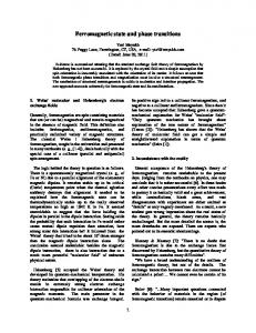
Fig. 2.1. Graph of the stress-strain relation σ for case (a) (left-hand figure) and case (b) (right-hand figure) from Assumption 2.3.

(b) The function σ is monotone increasing and there is a number α ∈ R such that σ 00 (w) < 0 for w ∈ (−∞, α) and σ 00 (w) > 0 for w ∈ (α, ∞) holds. The non-monotone shape of σ for case (a) in Assumption 2.3 allows to define different phases in the following way. The strain values in the interval (−∞, α1 ] are identified with a low-strain phase and strain values in the interval [α2 , ∞) with a high-strain phase. All other strain values are called elliptic. If Assumption (b) applies we associate with w ∈ (−∞, α) (w ∈ (α, ∞)) a low-strain phase (high-strain phase). In Fig. 2.1 we present the graphs of examples for the stress-strain function, together with the associated energies. We record some remarks for the first-order conservation law (1.1) that we obtain if we neglect the dissipative effects in (1.5), resp. (2.10). Let µ ¶ −v f (w, v) := (w, v) ∈ R2 . −σ(w) The eigenvalues λ∓ = λ∓ (v, w) and associated eigenvectors r∓ = r∓ (v, w) of the Jacobian of f are given by ¶ µ p 1 0 p λ∓ (v, w) = ∓ σ (w), r∓ (v, w) = , ± σ 0 (w) provided (w, v) ∈ R2 are such that σ 0 (w) ≥ 0 holds. Otherwise there are no real eigenvalues. Moreover we compute for the classification of the characteristic fields σ 00 (w) ∇λ∓ (v, w) · r∓ (v, w) = ∓ p σ 0 (w)

(w, v) ∈ R2 .

(2.13)

The (sign of the) expression ∇λ∓ ·r∓ generalizes the notions of convexity/concavity to a vector-valued function, here the flux f (see [14] for instance).

8

C. ROHDE

Let now Assumption 2.3(a) be true. From the calculations above we observe that the first-order system (1.1) is hyperbolic in the low and high strain phases (−∞, α1 ] ∩ [α1 , ∞) but not in (α1 , α2 ). Furthermore we note that there are unique numbers β1 , β2 ∈ R with β1 < β2 and σ(β1 ) = σ(β2 ) such that Z

β2 β1

σ(β) − σ(βi ) dβ = 0

(i = 1, 2).

(2.14)

These are the Maxwell states (see Fig. 2.1). For the case (b) the hyperbolic state space is the complete space R2 but the characteristic fields change their type in w = α according to (2.13) and the convex-concave behaviour of σ. But even in this case it makes sense to speak of different phases as defined above. 3. Dynamical Phase Boundaries and Non-Local Viscosity-Capillarity Profiles. In this section we prove that the system (1.5), (1.8) has special solutions which correspond to dynamical phase boundaries. Throughout the section we suppose that Assumption 2.3 (a) holds, i.e. σ has a non-monotone shape. Let us stress that all definitions, notations etc. are specialized to (1.1) or (1.5) and not meant to hold for general conservation laws. 3.1. Shock Waves and Phase Boundaries. We start to consider the first-order system (1.1). Let (w± , v± ) ∈ R2 , and s ∈ R be given. A function µ

w0 v0

¶

=

µ

w0 (x, t) v 0 (x, t)

¶

=

(

(w− , v− )T : x − st < 0, (w+ , v+ )T : x − st > 0,

(3.1)

is a shock-wave for (1.1) with speed s connecting the states (w− , v− ) and (w+ , v+ ) if the conditions −s(w+ − w− ) = v+ − v− , −s(v+ − v− ) = σ(w+ ) − σ(w− )

(3.2)

hold. A shock-wave with speed s connecting the states (w− , v− ) and (w+ , v+ ) is called a phase boundary for (1.1) if w− and w+ lie in different phases but not in the interval (α1 , α2 ). We note that (3.2) is nothing but the Rankine-Hugoniot relation. It ensures that each shock wave is a weak solution of (1.1), (1.2) with the jump initial datum w0 = w− , v0 = v− for x < 0 and w0 = w+ , w0 = v+ for x > 0. We classify shock waves according to the following definitions. A shock wave (w 0 , v 0 )T for (1.1) is called a Laxian or compressive shock wave if either λ− (w− , v− ) > s > λ− (w+ , v+ ) or λ+ (w− , v− ) > s > λ+ (w+ , v+ ) is satisfied. A shock wave (w 0 , v 0 )T for (1.1) is called an undercompressive shock wave if λ+ (w− , v− ) > s > λ− (w+ , v+ ) and λ+ (w+ , v+ ) > s > λ− (w− , v− ) is satisfied (see Fig. 3.1). Phase boundaries can be compressive or undercompressive. If the chord connecting the points (w± , σ(w± )) intersects the graph of σ in a third point they are undercompressive. Since these connections are close to the equilibrium configuration, i.e., the shock wave with speed zero connecting the states with w-component equal to the Maxwell states and vanishing v-component, it is believed that such waves are the physically most relevant ones ([1]). We will focus on this kind of phase boundaries in the sequel. Let us mention that undercompressvie waves have also been observed in the magnetohydrodyamics (see [23] for a review) and in the theory of thin films ([10, 11]).

9

Phase Transition and Non-local Energy

t

t s=

x t

s=

x t

(w+ , v+ ) (w− , v− )

(w+ , v+ ) x

(w− , v− )

x 0

0

(b) undercompressive shock wave

(a) Laxian shock wave

Fig. 3.1. Shock lines {(x, t) ∈ R × (0, ∞) | x = st} for shocks with speed s ∈ R and characteristic curves (dotted lines) in the (x, t)-plane. The two characteristic curves for a state (w − , v− ) are the lines with slopes 1/λ− (w− , v− ) and 1/λ+ (w− , v− ) intersecting the horizontal axis at some negative x-value. The two characteristic curves for a state (w+ , v+ ) are the lines with slopes 1/λ− (τ+ , v+ ) and 1/λ+ (w+ , v+ ) intersecting the horizontal axis at some positive x-value.

3.2. Non-Local Viscosity-Capillarity Profiles. We turn now to the non-locally regularized system (1.5), (1.8) and discuss the admissibility problem of undercompressive phase boundaries. For the sake of simplicity the capillarity constant γ is set to 1. Let (w± , v± ) ∈ R2 and s ∈ R be given such that (w 0 , v 0 ) from (3.1) is a shock-wave with speed s connecting the states (w− , v− ) and (w+ , v+ ). A function (w, v)T : R → R2 with w ∈ C 1 (R),

v ∈ C 2 (R)

is a non-local viscosity-capillarity profile for (w 0 , v 0 )T if it solves the differential-integro boundary value problem −sw − v = −sw− − v− ,

−(φ ∗ w − w) + µv˙ = −σ(w) − sv − (−σ(w− ) − sv− ) in R, w(±∞) = w± ,

(3.3)

v(±∞) = v± .

Here φ : R → [0, ∞) is an interaction potential as defined in (2.6) in the case of d = 1. For some given non-local viscosity-capillarity profile we have [φ ∗ w](x) − w(x) → 0 for x → ±∞ by using φ ∈ L1 (R) and Lebesgue’s theorem. Since w± , v± and s obey the Rankine-Hugoniot conditions (3.2) we see then that the states (w± , v± ) are rest points of the generalized flow associated with (3.3). From the definition of a viscosity-capillarity profile we deduce the following statement. Corollary 3.1. Let (w± , v± ) ∈ R2 and s ∈ R be given such that (w 0 , v 0 )T from (3.1) is a shockwave with speed s connecting the states (w− , v− ) and (w+ , v+ ). Assume that there exists a non-local viscosity-capillarity profile (w, v)T : R → R2 for the shock wave (w 0 , v 0 )T . Then for each ε > 0 the functions w ε ∈ C 1 (R × (0, T )) and v ε ∈ C 2 (R × (0, T )) defined by ¶ µ ¶ µ x − st x − st ε ε , v (x, t) = v ((x, t) ∈ R × (0, T )) w (x, t) = w ε ε are classical solutions of (1.5) with γ = 1. Moreover we have for almost all (x, t) ∈ R × (0, T ) wε (x, t) → w 0 (x, t),

v ε (x, t) → v 0 (x, t).

Proof. Straightforward calculation using (1.5), (1.8), (3.3), and the definition of the ε-scaled potential in (2.5).

10

C. ROHDE

We observe that admissibility of a shock wave in the sense of a non-local viscosity capillarity criterium means to prove the existence of a solution for the ε-independent problem (3.3). The ε-independence of (3.3) underlines that our conjecture on the ε-scaling between viscosity and capillarity terms in (1.5) is correct. Before we proceed let us put down the following useful consequence of (3.2). h(w+ , w− , s2 ) 0

h(r, r , q)

=

0,

:=

−(q(r − r 0 ) − σ(r) + σ(r 0 ))

(r, r 0 ∈ R, q ≥ 0) .

(3.4)

With (3.4) we can reduce the problem (3.3) to a first-order differential-integro problem for w alone: φ ∗ w − w + sµw˙ = h(w, w− , s2 ), w(±∞) = w± .

(3.5)

The velocity v is then determined from the first equation in (3.3). Our traveling-wave analysis relies on a result from [7] for general boundary value problems of type (3.5). We summarize what we need from this paper. Theorem 3.2 (Bates et al.). Let φ ∈ C r (R) ∩ W r,1 (R) for r ∈ N be an interaction potential in R. Let u− , u+ ∈ R and F ∈ C r (R) be given. For the unknowns u : R → R and ν ∈ R consider the problem φ ∗ u − u + ν u˙

=

F (u),

u(±∞)

=

u± .

(3.6)

We suppose that the states u± ∈ R and the function F satisfy (i)

u− > u+ ,

(ii)

F (u± ) = 0, F 0 (u± ) > 0,

(iii)

∃ ! u0 ∈ (u+ , u− ) : F (u0 ) = 0,

(iv)

u ∈ [u+ , u− ] ⇒ F 0 (u) + 1 > 0.

Then exactly one of the following statements holds true. (i) There is a monotonely decreasing function u ∈ C r+1 (R) and a unique ν ∈ R \ {0} such that (3.6) holds. In this case we have µZ ∞ ¶−1 Z u+ 2 F (u) du. (3.7) ν = H(u− , u+ ) (u(ξ)) ˙ dξ , H(u− , u+ ) := u−

−∞

(ii) There is a monotonely decreasing function u ∈ C r (R) such that (3.6) holds for ν = 0. In this case we have H(u− , u+ ) = 0.

(3.8)

In both cases the function v is unique up to translation. An analogous theorem holds for the inverse inequality in condition (i) of the last theorem. We present directly the following result on the existence of non-local profiles and recall the definition of the Maxwell states in (2.14). Theorem 3.3. Let φ ∈ C 1 (R) ∩ W 1,1 (R) be an interaction potential in R. Moreover suppose that σ satisfies Assumption 2.3(a), that 2σ 0 > −1 holds, and that σ 00 vanishes only at a finite number of

Phase Transition and Non-local Energy

points. Then there exists a number δ0 > 0 such that for all states ¯¯ ¯ ª © (w− , v− ) ∈ (w, v) ∈ (α2 , ∞) × R ¯ ¯σ(w) − σ(β1 )¯ < δ0

11

(3.9)

there exists a number µ > 0, a speed s ∈ R \ {0} and a state

(w+ , v+ ) ∈ (−∞, α1 ) × R with the properties (i) w± , v± , s satisfy the Rankine-Hugoniot condition (3.2), (ii) the phase boundary (w 0 , v 0 )T with speed s connecting (w− , v− ) with (w+ , v+ ) has a non-local viscosity-capillarity profile (w, v)T ∈ C 2 (R) × C 2 (R), (iii) the phase boundary (w 0 , v 0 )T is undercompressive. Before we prove Theorem 3.3 let us give some remarks on the statement. Note 3.4. (i) In Theorem 3.3 the left-hand state (w− , v− ) was chosen such that w− is located in the highstrain phase. Of course an analogous theorem holds for w− located in the low-strain phase. (ii) We get existence of non-local viscosity-capillarity profiles for dynamical phase boundaries that are undercompressive and have strain end states close to the Maxwell states. As we mentioned before such phase boundaries are expected to exist in reality. (iii) In this section we handled the case (a) in Assumption 2.3. In fact Theorem 3.2 can also be applied in the purely hyperbolic case (b) in Assumption 2.3. We refer to [38] for the detailed treatment of a closely related scalar problem. (iv) From Theorem 3.3 (in fact from 3.2) we observe that for a given phase boundary the existence of a viscosity-capillarity profile depends crucially on the viscosity coefficient µ which controls the ratio between viscosity and capillarity. Recall that the capillarity constant has been set to 1 in this section. This is in complete agreement with existence results for the local model (1.5), (1.7) and related systems. We refer to [8, 30, 42]. Proof of Theorem 3.3: For δ > 0 we define ¯¯ ¯ © ª Sδ := w ∈ (−∞, α1 ) ∪ (α2 , ∞) ¯ ¯σ(w) − σ(β1 )¯ < δ .

Furthermore we introduce for w1 , w2 ∈ R with w1 6= w2 the quantity q[w1 , w2 ] =

σ(w1 ) − σ(w2 ) . w1 − w 2

Now we choose δ0 > 0 so small such that we have for all w1 ∈ Sδ0 ∩ (α2 , ∞) and w2 ∈ Sδ0 ∩ (−∞, α1 ) the properties min{σ 0 (w1 ), σ 0 (w2 )} > q[w1 , w2 ], q[w1 , w2 ]
0 with these properties since we have £ ¤ q β1 , β 2 = 0

12

C. ROHDE

by construction of the Maxwell states in (2.14) and since the chord connecting (β 1 , σ(β1 )) with (β2 , σ(β2 )) intersects the graph of σ three times. Note moreover that Assumption 2.3(a) implies that the slope of σ close to the Maxwell states is bounded from below by a positive constant. Now according to the assumptions of the theorem we choose an arbitrary state (w− , v− ) ∈ (Sδ0 ∩ (α2 , ∞)) × R. Furthermore we take a number w ˜+ with w ˜+ ∈ Sδ0 ∩ (−∞, α1 ) and σ(w ˜+ ) < σ(w− ).

(3.13)

Consider the auxiliary problem to find µ ˜ ∈ R and w ∈ C 1 (R) such that φ∗w−w+µ ˜w˙

=

h(w, w− , q[w− , w ˜+ ]), w(−∞) = w− , w(∞) = w ˜+

(3.14)

holds. Note that q[w− , w ˜+ ] is positive due to (3.13). We apply Theorem 3.2 with F (w) = h(w, w− , q[w− , w ˜+ ]) to solve (3.14) and check conditions (i)-(iv). Condition (i) is clear since w− > w ˜+ by construction. The Rankine-Hugoniot relations (3.2) imply F (w− ) = F (w ˜+ ) = 0. We have for w ∈ R ∂ h(w, w− , q[w− , w ˜+ ]) = σ 0 (w) − q[w− , w ˜+ ]. ∂w The latter quantity is positive for w = w− , w ˜+ due to (3.10). Thus (ii) holds. Condition (iii) is a direct consequence of the definition of h (cf. (3.4)), (3.12) and the fact that σ 0 < 0 in (α1 , α2 ) due to Assumption 2.3(a). Using (3.11) we compute for w ∈ (w ˜ + , w− ) ∂ h(w, w− , q[w− , w ˜+ ]) + 1 = σ 0 (w) − q[w− , w ˜+ ] + 1 > σ 0 (w) + 1/2. ∂w The assumption σ 0 > −1/2 on the stress-strain relation assures condition (iv). We can apply Theorem 3.2 which tells us that there is a unique (up to translation) function w ∈ C 1 (R) and a unique number µ ˜ ∈ R that solves (3.14). In the next step we want to show that w ˜+ can be chosen such that µ ˜ 6= 0 holds. To determine the sign of µ ˜ it suffices by (3.7) and (3.8) to compute the sign of the term Z w˜+ H(w− , w ˜+ ) = h(w, w− , q[w− , w ˜+ ]) dw. w−

0

We obtain for some function W with W = −σ and (3.4) after straightforward calculations ¶ µ Z w˜+ W (w ˜+ ) − W (w− ) w ˜ + − w− −σ(w ˜+ ) − σ(w− ) − 2 h(w, w− , q[w− , w ˜+ ]) dw = 2 w ˜ + − w− w− =:

w ˜ + − w− G(w− , w ˜+ ). 2

To analyze the function G(w− , .) we compute µ ¶ d −2 1 00 2 0 G(w− , w) = W (w− ) − W (w) − W (w)(w− − w) − W (w)(w− − w) 2 dw 2 (w − w− ) Z w− −1 = σ 00 (z)(w− − z)3 dz. 3(w − w− )2 w

Phase Transition and Non-local Energy

13

The preceding computation and the assumption that σ 00 vanishes only in finitely many points implies the following. If G(w− , .) vanishes in w ˜+ and thus we have µ ˜ = 0 in (3.14) there is a specific volume w+ ∈ Sδ0 ∩ (−∞, α1 ) close to w ˜+ with σ(w+ ) < σ(w− ).

(3.15)

such that G(w− , w+ ) does not vanish. In this degenerate case we take the new specific volume w + (and let it as it was if G(w− , .) does not vanish in w ˜+ ) as a new end state in (3.14). By repeating all arguments above with the new end state and applying Theorem 3.2 we obtain a solution (˜ µ, w) ∈ R \ {0} × C 2 (R) of (3.14). In the final step we construct a solution of the original problem (3.5) by s |˜ µ| σ(w− ) − σ(w+ ) , µ := . s := sgn(˜ µ) w− − w + |s| To fulfill the Rankine-Hugoniot conditions for the velocity components we set v+ = v− − s(w+ − w− ). Note that v− was given. We have proven (ii). By construction it is clear that also (i) holds. Moreover (iii) is true since the condition (3.12) is true for w1 = w− and w2 = w+ and implies that the associated shock wave (w 0 , v 0 )T is undercompressive (see discussion at the end of Sect. 3.1). 2 4. The Sharp Interface Limit for a General Cauchy Problem. In this section we do not consider special solutions of (1.5), (1.6) and consider the sharp-interface limit for these solutions as in Sect. 3. Rather we consider (quite) general initial data for the Cauchy problem (1.5), (1.6) where σ ic chosen according to Assumption 2.3(b). In this case we show that a sequence of classical solutions for (1.5), (1.6) converges to a weak solution of (1.1) (Theorem 4.5). Even if one cannot say anything on the structure of this weak solutions the result underlines that the chosen ε-scaling is correct and leads to a well-defined limit-process. We will first collect some preliminaries in Sect. 4.1, present the crucial ε-independent estimates in Sect. 4.2, and state and prove the main theorem in Sect. 4.3. Let us note that the analogous analysis for the local version (1.5), (1.7) has been performed in [29]. 4.1. Global Existence of Classical Solutions for the Non-Local Model. We consider the Cauchy problem for (1.5), (1.6). For the rest of this section we suppose that initial data, kernel functions, and stress-strain relations are chosen according to the following assumption. Assumption 4.1. (i) The stress-strain function σ satisfies Assumption 2.3(b) with α = 0 and fulfills σ 00 , σ 000 ∈ L1 (R) ∩ L∞ (R), σ(0) = 0. Moreover there are constants a, A > 0 such that we have for all w ∈ R a ≤ σ 0 (w) ≤ A. (ii) The interaction potential φ in R is in C 1 (R) and satisfies supp(φ) ∈ [−1, 1]. The function φε is given by (2.5) for d = 1.

14

C. ROHDE

(iii) The initial functions w0 , v0 belong to C 1 (R) and satisfy w0 , w0x , v0 ∈ L2 (R).

(4.1)

A consequence of Assumption 4.1(ii),(iii) is that we have for all ε > 0 the estimate Z

R

E ε [w0 ](x) dx < γkw0 kL2 (R) < ∞.

Here the mapping E ε : L2 (R) → L1 (R) is given by E ε [w](x) =

γ 4

Z

R

¡ ¢2 φε (x − y) w(y) − w(x) dy

(w ∈ L2 (R), x ∈ R).

(4.2)

The conditions on the stress-strain relation σ in Assumption 4.1 look quite restrictive. We have chosen them in way such that the theory of compensated compactness as developped by Serre and Shearer applies ([40]). For us the important point is that σ is not convex. This allows still the construction of undercompressive shock waves for the first-order system (1.1) which have physical relevance ([29]). Finally we note that the choice α = 0 is no restriction but only a simplification of notation. The analysis holds for arbitrary position of the inflection point. For T > 0 let the set C12 (R × (0, T )) denote the set of real-valued functions on R × [0, T ] such that all spatial derivatives up to order 2 and the first-order time derivative is continuous in R × (0, T ). By a classical solution of (1.5), (1.6) we mean a function (w ε , v ε )T ∈ (C12 (R × (0, T )))2 such that (1.5) and (1.6) hold pointwise. We need the existence of a sequence {(w ε , v ε )}ε>0 of classical solutions of the Cauchy problem for (1.5) to analyze the limit behaviour for ε → 0. We make the following assumption on the existence of classical solutions. Assumption 4.2. For each ε > 0 there exists a unique classical solution (w ε , v ε )T ∈ (C12 (R × (0, T )))2 of (1.5), (1.6) with wε , v ε , wxε ∈ C([0, T ]; L2 (R)),

w ε , v ε ∈ C12 (R × (0, T )).

The classical solution satisfies for t ∈ (0, T ] ε (., t) ∈ L2 (R). vxε (., t), wtε (., t), wxx

As a consequence of Assumption 4.2 we have for t ∈ (0, T ] the decay properties lim

|x|→∞

³

´ |wε (x, t)| + |wxε (x, t)| + |v ε (x, t)| + |vxε (x, t)| = 0.

(4.3)

Since the term (1.8) is of first order we can absorb it into the flux term −σ(w) x in (1.5) and obtain a problem that has formally the structure of a hyperbolic-parabolic problem like (1.5), (1.6) with γ = 0. For the latter case the existence of classical solutions for an initial boundary value problem under Assumption 4.1 has been proven in [25] (see also [6]). We conjecture that this result can be extended to our case if one considers the non-local capillarity term as a contribution to the flux. Since we are not interested in the case for positive but fixed value for ε we do not give the proof of this statement but focus on the limit process ε → 0. We note that the existence of weak solutions for (1.5), (1.6) under Assumption 4.1 has been shown in [39].

Phase Transition and Non-local Energy

15

4.2. Estimates independent of ε. The first step to the convergence statement is an estimate on the family {(w ε , v ε )}ε>0 of classical solutions which is uniform with respect to the regularization parameter ε. We obtain this estimate only in terms of some Lp -norms with p 6= ∞. For system (1.5) and also its local counterpart global-in-time L∞ -estimates independent of ε are not available. These have only be derived for systems equipped with additional non-physical viscosity (see e.g. [15]). The estimate rather exploits the properties of the physical energy H ∈ C 4 (R2 ) given by H(w, v) =

v2 + W (w) 2

˜ ∈ C 4 (R) is defined by Here the function W W (w) =

Z

(v, w ∈ R).

w

σ(w) ˜ dw ˜ w0

(w ∈ R),

which leads by Taylor expansion and Assumption 4.1(i) to the estimate 0
0 of classical solutions of (1.5), (1.6) and a function (w, v)T ∈ L2 (R × (0, T )) × L2 (R × (0, T )) such that (i) the subsequence converges for k → ∞ to (w, v)T in (Lqloc (R × (0, T )))2 , q ∈ [1, 2), (ii) (w, v)T is a weak solution of (1.1), i.e., ¶ µ ¶ Z TZ µ w(x, t) v(x, t) ψt (x, t) − ψx (x, t) dxdt = 0 (4.10) v(x, t) σ(w(x, t)) 0 R for all ψ ∈ C0∞ (R × (0, T )). Before we can present the proof of Theorem 4.5 we need the following lemma. Lemma 4.6. Let the assumptions of Theorem 4.5 be valid. Then there exists a constant C > 0 independent of ε such that kφε ∗ wε − wε kL2 (R×(0,T )) ≤ Cεkwxε kL2 (R×(0,T )) . Proof. Let (x, t) ∈ R × (0, T ) be arbitrary but fixed. Denote Bε (x) = {y ∈ R | |x − y| ≤ ε}. We consider I : R × (0, T ) → R with Z I(x, t) = [φε ∗ wε (., t)](x) − w ε (x, t) = φε (x − y)(w ε (x, t) − w ε (y, t)) dy. R

18

C. ROHDE

Assumption 4.1(ii) and the Morrey-type inequality (see Sect. 5.6.2 of [18]) √

|w(x) − w(y)| ≤ C1 ε

µZ

x+2ε 2

|wx (z)| dz

x−2ε

¶1/2

(x ∈ R, y ∈ Bε (x), w ∈ C 1 (R))

show that the following estimate holds. Z φε (x − y)|(w ε (x, t) − w ε (y, t))| dy |I(x, t)| ≤ Bε (x)

≤ =

√ C1 ε √ C1 ε

Z

φε (x − y)

Bε (x) µZ x+2ε x−2ε

µZ

x+2ε

|wxε (z, t)|2 dz

x−2ε ¶1/2

|wxε (z, t)|2 dz

¶1/2

dy

.

z) Now we integrate |I(x, t)|2 with respect to space and obtain with the substitution z = x + 4ε π arctan(˜ ¶ Z Z µZ x+2ε |wxε (z, t)|2 dz dx |I(x, t)|2 dx = C1 ε x−2ε R R Z µZ ¯ ³ ´¯2 ¶ 4ε 1 4ε ¯ ¯ ε arctan(˜ z ), t d˜ z = C1 ε w x + ¯ dx ¯ x π π 1 + z˜2 R R ¶ Z µZ 1 4ε2 = C1 |wxε (x, t)|2 dx d˜ z π R 1 + z˜2 R 2 ≤ C2 ε2 kwxε (., t)kL2 (R) . Integration with respect to time yields the statement of the lemma. We conclude the paper with the Proof of Theorem 4.5. From Lemma 4.4 we know that the family {(w ε , v ε )T }ε>0 of classical solutions of (1.5), (1.6) is in particular uniformly bounded in L2 (R × (0, T )) × L2 (R × (0, T )). We shall now show that the inclusion η(wε , v ε )t + q(wε , v ε )x ⊂ compact set in W −1,2 (Q) + bounded set in M(Q)

(4.11)

holds for all open bounded sets Q ⊂ R × (0, T ) and two special entropy pairs (η, q) ∈ C 2 (R2 , R2 ) for (1.1) that have been constructed in [41]. Then the Lemma of Murat ([36]) and the theorem of Shearer and Serre (see [35] for instance) apply: Statement (i) follows. We have to establish (4.11). We do not give the exact formulae for the Shearer entropies which can be found in [41]. For our purposes it suffices to note that there is a constant C > 0 such that the entropies of a Shearer entropy pair (η, q) satisfy the estimates √ √ kηw / σ 0 kL∞ (R2 ) + kηv kL∞ (R2 ) + kηwv / σ 0 kL∞ (R2 ) + kηww /σ 0 kL∞ (R2 ) + kηvv kL∞ (R2 ) < C. (4.12) Let such an entropy pair be given. We compute with (1.5) η(wε , v ε )t + q(wε , v ε )x

= =:

¡ ¢ ε εηv (wε , v ε )vxx + γηv (wε , v ε ) φε ∗ wε − wε x

I1ε + I2ε .

In the sequel let θ ∈ W01,2 (Q) and ψ ∈ C0∞ (Q). We start with the term I1ε which we rewrite in the form I1ε

= =:

ε εη(wε , v ε )xx − ε(wε , v ε )∇2 η(wε , v ε )(wε , v ε )T − εηw (wε , v ε )wxx

ε ε ε I11 + I12 + I13 .

Phase Transition and Non-local Energy

19

The terms can be treated exactly as in [41] and one obtains using (4.12) for some ε-independent constant C12 > 0 ε ε , ψi| ≤ C12 kψkL∞ (Q) . , θi| = 0 and |hI12 lim |hI11

ε→0

(4.13)

ε To work out the term I13 we take into account the splitting ε ε ε + I132 = ε(ηw (wε , v ε )wxε )x − ε∇ηw (wε , v ε ) · (wxε , vxε )T wxε =: I131 I13

and compute with (4.12) and Lemma 4.4 ¯Z ¯ ¯ ¯ ε |hI131 , θi| = ε¯ ηw (wε (x, t), v ε (x, t))wxε (x, t)θx (x, t) dxdt¯ Q p = εC131 k σ 0 (wε )wxε kL2 (Q) kθkW 1,2 (Q) → 0

(4.14)

(ε → 0).

ε Furthermore, for I132 we estimate ¯Z ¡ ¯ ε |hI132 , ψi| = ε¯ ηww (wε (x, t), v ε (x, t))wxε (x, t) Q

≤ ≤ ≤

¯ ¢ ¢ ¯ +ηvw (wε (x, t), v ε (x, t))vxε (x, t) wxε (x, t) ψ(x, t) dxdt¯ ¯ ¯Z ¯ ¯ 2σ 0 (wε (x, t))(wxε (x, t))2 + vxε (x, t) dxdt¯ C132 ε¯ Q ¡ p ¢ 2 2 C132 ε k σ 0 (wε )wxε kL2 (Q) + kvxε kL2 (Q) kψkL∞ (Q)

(4.15)

C132 kψkL∞ (Q) .

We proceed with I2ε which we split up according to µ µ µ µ ε¶ µ ¶ ¶ 0 wx 0 2 ε ε I2ε = γ ∇η(wε , v ε ) · − γ ∇ η(w , v ) · φε ∗ w ε − w ε x vxε φε ∗ w ε − w ε =:

ε ε I21 + I22 .

Here ∇2 η is the Hessian matrix of the entropy η. Using Lemma 4.6 and again (4.12), Lemma 4.4 leads to ¯Z ¯ ¡ ¢ ¯ ¯ ε |hI21 , θi| = γ ¯ ηv (wε (x, t), v ε (x, t)) [φε ∗ wε (., t)](x) − w ε (x, t) θx (x, t) dxdt¯ Q

≤

C21 γkφε ∗ wε − wε kL2 (Q) kθkW 1,2 (Q)

→

0

(4.16)

(ε → 0)

and ε , ψi| |hI22 ¯Z ¯ ¡ ¢ ¯ ¯ = γ¯ ηwv (wε (x, t), v ε (x, t))wxε (x, t) [φε ∗ wε (., t)](x) − w ε (x, t) ψ(x, t) dxdt¯ Q ¯ ¯Z ¡ ¢ ¯ ¯ ηvv (wε (x, t), v ε (x, t))vxε (x, t) [φε ∗ wε (., t)](x) − w ε (x, t) ψ(x, t) dxdt¯ + γ¯ Q ´ ³ p ≤ C22 γ k σ 0 (wε )wxε kL2 (Q) + kvxε kL2 (Q) kφε ∗ wε − wε kL2 (Q) kψkL∞ (Q)

≤

C22 γkψkL∞ (Q) .

(4.17)

20

C. ROHDE

Collecting the results from (4.13) ,(4.14), (4.15), (4.16), and (4.17) we observe that (4.11) holds. We proceed with statement (ii). Since the elements of the converging subsequence {(w εk , v εk )T }k∈N are classical solutions of (1.5), (1.6) we have for k ∈ N and for all ψ ∈ C0∞ (R × (0, T )) also ¶ µ ¶ Z T Z µ εk w (x, t) v εk (x, t) ψ (x, t) − ψx (x, t) dxdt t v εk (x, t) σ(wεk (x, t)) 0 R ¶ Z TZ µ 0 (4.18) ψxx (x, t) dxdt = − εk v εk (x, t) 0 R ¶ Z TZ µ 0 ψx (x, t) dxdt. −γ [φεk ∗ wεk (., t)](x) − w εk (x, t) 0 R Since all expressions on the left-hand side of (4.18) are globally Lipschitz-continuous in v εk and wεk (recall Assumption 4.1(i) for σ) the convergence of {(w εk , v εk )T }k∈N in (Lqloc (R × (0, T )))2 , q < 2, implies convergence to the left-hand side of (4.10). The same argument shows that the first term on the right-hand side of (4.18) vanishes as εk → 0. Finally the last term term on the right-hand side of (4.18) vanishes due to Lemma 4.6 and Lemma 4.4. 2 REFERENCES [1] R. Abeyaratne and J. K. Knowles. Kinetic relations and the propagation of phase boundaries in solids. Arch. Ration. Mech. Anal., 114(2):119–154, 1991. [2] R. Abeyaratne and J.K. Knowles. Implications of viscosity and strain gradient effects for the kinetics of propagating phase boundaries in solids. SIAM J. Appl. Math., 51:1205–1221, 1991. [3] M. Affouf and R. Caflish. A numerical study of Riemann problem solutions and stability for a system of viscous conservation laws of mixed type. SIAM J. Appl. Math., 51:605–634, 1991. [4] G. Alberti and G. Bellettini. A non-local anisotropic model for phase transitions: Asymptotic behaviour of rescaled energies. Eur. J. Appl. Math., 9(3):261–284, 1998. [5] G. Alberti, G. Bellettini, M. Cassandro, and E. Presutti. Surface tension in Ising systems with Kac potentials. J. Stat.Phys., 82(3/4):743–793, 1996. [6] G. Andrews. On the existence of solutions to the equation utt = uxxt + σ(ux )x . J. Differential Equations., 35:200–231, 1980. [7] P.W. Bates, P.C. Fife, X. Ren, and X. Wang. Traveling waves in a convolution model for phase transitions. Arch. Ration. Mech. Anal., 138:105–136, 1997. [8] N. Bedjaoui and P.G. LeFloch. Diffusive-dispersive traveling waves and kinetic relations. II: An hyperbolic elliptic model of phase transitions. Proc. Royal Soc. Edinburgh, 132(3):545–565, 2002. [9] S. Benzoni-Gavage. Stability of subsonic planar phase boundaries in a van der Waals fluid. Arch. Ration. Mech. Anal., 150:23–55, 1999. [10] A. Bertozzi, A. M¨ unch, and M. Shearer. Undercompressive shocks in thin film flows. Physica D, 134(4):431–464, 1999. [11] A. Bertozzi and M. Shearer. Existence of undercompressive traveling waves in thin film equations. SIAM J. Math. Anal., 32(1):194–213, 2000. [12] J. Carr, M.E. Gurtin, and M. Slemrod. Structured phase transitions on a finite interval. Arch. Ration. Mech. Anal., 86:317–351, 1984. [13] R.M. Colombo and A. Corli. Continuous dependence in conservation laws with phase transitions. SIAM J. Math. Anal., 31(1):34–62, 1999. [14] C.M. Dafermos. Hyperbolic conservation laws in continuum physics. Springer-Verlag, New York, 2000. [15] R DiPerna. Convergence of approximate solutions to conservation laws. Arch. Ration. Mech. Anal., 82:27–70, 1983. [16] J. Ericksen. Equilibrium of bars. J. Elasticity, 5:191–201, 1975. [17] J. Ericksen. Constitutive theory for some constrained elastic crystals. J. Solids abd Structures, 22:951–964, 1986. [18] L.C. Evans. Partial Differential Equations. American Mathematical Society, Providence, R.I., 1998. [19] H. Fan. A vanishing viscosity approach on the dynamics of phase transitions in van der Waals fluids. J. Differ. Equations, 103(1):179–204, 1993. [20] H. Fan and M. Slemrod. Dynamic flows with liquid/vapor phase transitions. In S. Friedlander and D. Serre (eds.), Handbook of Mathematical Fluid Mechanics, pages 373–420. Elsevier Science, 2002.

Phase Transition and Non-local Energy

21

[21] P. Fife. Some nonclassical trends in parabolic and parabolic-like evolutions. In M. Kirkilionis, S. Kr¨ omker, R. Rannacher, and F. Tomi (eds.), Trends in Nonlinear Analysis, pages 153–178. Springer, 2003. [22] R. Fosdick and D. Mason. On a model of nonlocal continuum mechanics, Part 1: existence and regularity. SIAM J. Appl. Math., 54(4):1278–1306, 1998. [23] H. Freist¨ uhler, C. Fries, and C. Rohde. Existence, bifurcation, and stability of profiles for classical and non-classical shock waves. In B. Fiedler (ed.), Ergodic Theory, Analysis, and Efficient Simulation of Dynamical Systems, pages 287–310. Springer, 2001. [24] H. Gajewski and K. Zacharias. On a nonlocal phase separation model. J. Math. Anal. Appl., 286(1):11–13, 2003. [25] J.M Greenberg, R.C. MacCamy, and V.J. Mizel. On the existence, uniqueness, and stability od solutions of the equation σ 0 (ux )uxx + λuxtx = ρ0 utt . J. Math. Mech., 17:707–728, 1968. [26] R. Hagan and M. Slemrod. The viscosity-capillarity criterion for shocks and phase transitions. Arch. Ration. Mech. Anal., 83:333–361, 1983. [27] H. Hattori. The entropy rate admissibility criterion and the entropy condition for a phase transition problem: The isothermal case. SIAM J. Math. Anal., 31(4):791–820, 2000. [28] B.T. Hayes and P.G. LeFloch. Non-classical shocks and kinetic relations: Scalar conservation laws. Arch. Ration. Mech. Anal., 139(1):1–56, 1997. [29] B.T. Hayes and P.G. LeFloch. Nonclassical shocks and kinetic relations: strictly hyperbolic systems. SIAM J. Math. Anal., 31:941–991, 2000. [30] D. Jacobs, W. McKinney, and M. Shearer. Travelling wave solutions of the modified Korteweg-deVries-Burgers equation. J. Differ. Equations, 116(2):448–467, 1995. [31] R.D. James. The propagation of phase boundaries in elastic bars. Arch. Ration. Mech. Anal., 73:125–158, 1980. [32] J.K. Knowles. Impact-induced tensile waves in a rubberlike material. SIAM J. Appl. Math., 62(4):1153–1175, 2002. [33] P.G. LeFloch. Propagating phase boundaries: Formulation of the problem and existence via the glimm method. Arch. Ration. Mech. Anal., 123(2):153–197, 1993. [34] P.G. LeFloch. Hyperbolic systems of conservation laws. The theory of classical and nonclassical shock waves. Lectures in Mathematics, ETH Z¨ urich. Basel, 2002. [35] Y. Lu. Hyperbolic Conservation Laws and the Compensated Compactness Method. Chapman&Hall/CRC, 2003. [36] F. Murat. L’injection du cˆ one positif de H−1 dans W−1,q est compacte pour tout q < 2. J.Math.Pures Appl., 60:309–322, 1981. [37] R. Rogers and L. Truskinovsky. Discretization and hysteresis. Physica B, 233:370–375, 1997. [38] C. Rohde. Scalar conservation laws with mixed local and non-local diffusion-dispersion terms. Technical report, Math. Institut, Albert-Ludwigs-Universit¨ at Freiburg No. 18, 2003. submitted to SIAM J. Math. Anal. [39] C. Rohde and M.D. Thanh. Global existence for phase transition problems via a variational scheme. Technical report, Math. Inst., Universt¨ at Freiburg No. 31, 2004. accepted for publication in J. Hyperbolic Equations. [40] D. Serre and J. Shearer. Convergence with physical viscosity for nonlinear elasticity. Technical report, 1993. [41] J. Shearer. Global existence and compactness in l p for the quasilinear wave equation. Comm. Partial Diff. Eqs., 19:1829–1877, 1994. [42] M. Slemrod. Admissibility criteria for propagating phase boundaries in a van der Waals fluid. Arch. Ration. Mech. Anal., 81:301–315, 1983. [43] L. Truskinovsky. Kinks versus shocks. In J.E. Dunn, R. Fosdick, and M. Slemrod (eds.), Shock induced transitions and phase structures in general media, pages 185–229. Springer, 1993.