Phase transitions in evolutionary dynamics - bioRxiv

bioRxiv preprint first posted online Jul. 3, 2018; doi: http://dx.doi.org/10.1101/361337. The copyright holder for this preprint (which was not peer-reviewed) is the author/funder. It is made available under a CC-BY 4.0 International license.

Phase transitions in evolutionary dynamics ´ Fernando Alcalde Cuesta1,5 , Pablo Gonz´alez Sequeiros2,5 , Alvaro Lozano Rojo3,4,5 1 Departamento de Matem´aticas, Universidade de Santiago de Compostela, E-15782 Santiago de Compostela, Spain 2 Departamento de Did´acticas Aplicadas, Facultade de Formaci´ on do Profesorado, Universidade de Santiago de Compostela, Avda. Ram´on Ferreiro s/n, E-27002 Lugo, Spain 3 Centro Universitario de la Defensa, Academia General Militar, Ctra. Huesca s/n. E-50090 Zaragoza, Spain 4 IUMA, Universidad de Zaragoza, Pedro Cerbuna 12, E-50009 Zaragoza, Spain 5 GeoDynApp - ECSING Group, Spain

Abstract The evolutionary dynamics of a finite population where resident individuals are replaced by mutant ones depends on its spatial structure. The population adopts the form of an undirected graph where the place occupied by each individual is represented by a node and it is bidirectionally linked to the places that can be occupied by its clonal offspring. There are undirected graph structures that act as amplifiers of selection increasing the probability that the offspring of an advantageous mutant spreads through the graph reaching any node. But there also are undirected graph structures acting as suppressors of selection where, on the contrary, the fixation probability of an advantageous mutant is less than that of the same individual placed in a homogeneous population. Here, we show that some undirected graphs exhibit phase transitions between both evolutionary regimes when the mutant fitness varies. Firstly, as was already observed for small order random graphs, we show that most graphs of order 10 or less are amplifiers of selection or suppressors that become amplifiers from a unique transition phase. Secondly, we give examples of amplifiers of order 7 that become suppressors from some critical value. For graphs of order 6 and 7, we apply computer aided techniques to exactly determine their fixation probabilities and then their evolutionary regimes, as well as the exact critical values for which each graph changes its regime. A similar technique is used to explore a general method to suppress selection in bigger orders, namely from 8 to 15, up to some critical fitness value. The analysis of all graphs from order 8 to order 10 reveals a complex and rich evolutionary dynamics, which have not been examined in detail until now, and poses some new challenges in computing fixation probabilities and times of evolutionary graphs.

Introduction In recent times the evolutionary theory on graphs has become a key field to understand biological systems. Although evolutionary dynamics has been classically studied for homogeneous populations, there is now a wide interest in the evolution of populations arranged on graphs after mutant spread. The process transforming nodes occupied by residents into nodes occupied by mutants is described by the Moran model. Introduced by Moran [1] as the Markov chain that counts the number of invading mutants in a homogeneous population, it was adapted to subdivided population by Maruyama [2, 3] and rediscovered by Lieberman et al. [4] for general graphs. For undirected graphs where links have no orientation, mutants will either become extinct or take over the whole population, reaching one of the two absorbing states, extinction or fixation. The fixation probability is the fundamental quantity in the stochastic evolutionary analysis of a finite population. If the population is homogeneous, at the beginning, one single node is chosen at random to be occupied by a mutant individual among a population of N resident individuals. Afterwards, an individual is randomly chosen for reproduction, with probability proportional to its reproductive advantage (1 for residents and

1

bioRxiv preprint first posted online Jul. 3, 2018; doi: http://dx.doi.org/10.1101/361337. The copyright holder for this preprint (which was not peer-reviewed) is the author/funder. It is made available under a CC-BY 4.0 International license.

r ≥ 1 for mutants), and its clonal offspring replaces another individual chosen at random. In this case, the fixation probability is given by Φ0 (r) =

rN −1 1 − r−1 = N −1 . −N N 1−r r + r −2 + · · · + r + 1

(1)

If the population is arranged on nodes of an undirected graph, the replacements are limited to the nodes that are connected by links. According to the Isothermal Theorem P[2–4], the fixation probability Φ(r) = Φ0 (r) if and only if the graph is isothermal (i.e. the temperature Ti = j∼i 1/dj of any node i is constant, where j is a neighbor of i and dj is the number of neighbors of j), or equivalently regular (i.e. the degree di of any node i is constant). But there are graph structures altering substantially the fixation chances of mutant individuals depending on their fitness. As showed in [4], there are graph structures that amplify this advantage. This means the fixation probability function Φ(r) > Φ0 (r) for all r > 1 for the same order N . Notice that Φ(1) = 1/N and the inequality must be reversed for r < 1. Due to the exact analytical computation of Φ(r) given by Monk et al. [5], it is known that star and complete bipartite graphs are amplifiers of natural selection whose fixation functions are bounded from above by Φ2 (r) = Φ0 (r2 ) =

1 − r−2 . 1 − r−2N

(2)

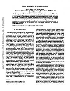
On the other hand, there are also graph structures that suppress the reproductive advantage of mutant individuals so that Φ(r) < Φ0 (r) for all r > 1. Examples of this kind of graph structures were known for some fitness values (see [6]). In [7], we introduced examples of suppressors of natural selection of order 6, 8 and 10 (see Fig 1), denoted by `6 , `8 and `10 , whose fixation probabilities remain smaller than Φ0 (r) for every r > 1.

`6 `8 `10 Fig 1. Suppressors of order 6, 8 and 10 for any fitness value. In [7], we called `-graph the undirected graph of even order N = 2n + 2 ≥ 6 obtained from the clique K2n by dividing its vertex set into two halves with n ≥ 2 vertices and adding 2 extra vertices. Each of them is connected to one of the halves of K2n and with the other extra vertex. The analysis of disadvantageous mutants (with r < 1) is also interesting when comparing amplification and suppression of selection for graphs, but here, for simplicity, we focus on the case of advantageous mutant (with r > 1). Different initialization and updating types have been also considered in [8] and [9], see also [10] for a comparative analysis of update mechanisms. If the initial distribution is uniform (i.e. the probability that a node will be occupied by the initial mutant is equal for all the nodes) and the graph evolves under Birth-Death updating, Hindersin and Traulsen showed in [9] that almost all small undirected graphs are amplifiers of selection. Assuming both conditions and focusing on the advantageous case, we distinguish two different evolutionary regimes out of the isothermal one: given values 1 ≤ r0 < r1 ≤ +∞, a graph is an amplifier of selection for r ∈ (r0 , r1 ) if the fixation probability function Φ(r) > Φ0 (r) and a suppressor of selection for r ∈ (r0 , r1 ) if Φ(r) < Φ0 (r) for all r0 < r < r1 . Star and bipartite complete graphs are amplifiers for r ∈ (1, +∞) and graphs `6 , `8 and `10 are suppressors for r ∈ (1, +∞). There are suppressors that become amplifiers from some critical value rc > 1 (see Fig 2). Borrowing the terminology from percolation theory, in this case, we say rc is a transition phase from the suppressor regime to the amplifier regime. In general, we say that a number rc > 1 is a transition phase between two different evolutionary regimes if there are values 1 ≤ r0 < r1 ≤ +∞ such that the graph is a suppressor (resp. an amplifier) for r ∈ (r0 , rc ) and an amplifier (resp. a suppressor) for r ∈ (rc , r1 ).

2

bioRxiv preprint first posted online Jul. 3, 2018; doi: http://dx.doi.org/10.1101/361337. The copyright holder for this preprint (which was not peer-reviewed) is the author/funder. It is made available under a CC-BY 4.0 International license.

(A)

Id 17451461644

Id 406331401

(B)

Id 1151997057027

Id 1151994460194

Fig 2. Suppressors that become amplifiers. (A) Examples of order 6 from [11] with a unique transition phase at rc ≈ 2.82 and rc ≈ 4.56 respectively. (B) Examples of order 7 from [6] having a unique transition phase at rc ≈ 79.15 and rc ≈ 1.98 respectively. In both cases, we use identification numbers from [11]. In this paper, we show that most graphs of order 10 or less are amplifiers or suppressors that become amplifiers from a unique transition phase rc > 1. However, we also exhibit two other types of transitions which are much more interesting: • There are amplifiers of order greater or equal to 7 that become suppressors from a unique transition phase rc > 1. • There are graphs of order greater or equal to 8 exhibiting more than one transition phase. Since the fixation probabilities Φ0 (r) and Φ(r) are monotonically increasing, these results were not exactly expected, while numerical simulations should be considered with caution. In fact, for finite populations, it has been suggested that results obtained for weak selection may remain valid when the selection is no longer weak. However, in [12], Wu et al. showed that this is no the case for homogeneous populations under frequency dependent selection. Here, we show that the graph structure can completely alter the evolutionary regime of a structured population even under constant selection. In addition, the fact that the survival chances of mutant individuals may decrease with respect to a homogeneous population when their fitness increases might have interesting biological consequences. Our results also demonstrate that numerical simulation is not enough to determine the evolutionary regime of a graph for the whole range of fitness values. Moreover, the very slight difference between different regimes for some graphs often forces to consider an extremely high number of trials when using Monte Carlo method, like recently in [13] to show a family of graphs of order ≥ 12 that changes from amplifier to suppressor as r increases. For example, 1010 trials were needed in [7] to determine the evolutionary regime of the graphs `N for 12 ≤ N ≤ 24 and 1 ≤ r ≤ 4. In [11], we presented an extremely precise database of fixation probabilities for all undirected graphs of order 10 or less for fitness values r varying from 0.25 to 10 with step size of 0.25 (see details in Materials and Methods). Here, we use this database to detect new evolutionary dynamics: in this way, we identify two amplifiers of order 7 with a transition to the suppressor regime at some rc ≤ 10. Then we adapt the technique described in [7] to symbolically compute the exact fixation probability Φ(r) of these examples for all r > 1 proving that they really have a unique transition phase. A similar procedure is used to exactly determine the evolutionary regime of any graph of order 7 or less for any fitness value. Thus, we find a third example of order 7 exhibiting a transition from the amplifier to the suppressor regime for rc > 10. The first

3

bioRxiv preprint first posted online Jul. 3, 2018; doi: http://dx.doi.org/10.1101/361337. The copyright holder for this preprint (which was not peer-reviewed) is the author/funder. It is made available under a CC-BY 4.0 International license.

method is also applied to show the existence of graphs of order 8, 9 and 10 with more than one transition phase. This reveals that undirected graphs have a complex and rich evolutionary dynamics that are worth studying in detail.

Materials and Methods Mathematical model Let G be an undirected graph with node set V = {1, . . . , N }. In fact, all graphs considered here will be assumed connected. Denote by di the degree of the node i. The Moran process on G is a Markov chain Xn whose states are the sets of nodes S inhabited by mutant individuals at each time step n. The transition probabilities are obtained from the matrix W = (wij ) given by wij = 1/di if i and j are neighbors and wij = 0 otherwise. More precisely, for each fitness value r > 0, the transition probability between S and S 0 is given by  P r i∈S wij   if S 0 \ S = {j},   w (r)  S   P   i∈V \S wij  if S \ S 0 = {j}, wS (r) PS,S 0 (r) = (3) P P   r w + w  ij ij i,j∈S i,j∈V \S   if S = S 0 ,   wS (r)    0 otherwise, where wS (r) = r

XX

wij +

i∈S j∈V

X X

wij = r|S| + N − |S|

(4)

i∈V \S j∈V

is the total reproductive weight of resident and mutant individuals. The fixation probability of each subset S ⊂ V inhabited by mutant individuals ΦS (r) = P[ ∃n ≥ 0 : Xn = V | X0 = S ]

(5)

is a solution of the system of 2N linear equations ΦS (r) =

X

PS,S 0 ΦS 0 (r)

(6)

S0

with boundary conditions Φ∅ (r) = 0 and ΦV (r) = 1. The (average) fixation probability is given by Φ(r) =

N 1 X Φ{i} (r). N i=1

Denoting by P (r) = (PS,S 0 (r)) the transition matrix, Eq 6 can be written as       1 0 0 0 0        P (r) · Φ(r) =   b(r) Q(r) c(r)  · Ψ(r) = Ψ(r) = Φ(r), 1 1 0 0 1

(7)

(8)

where Φ(r) = (0, Ψ(r), 1) is the vector with coordinates ΦS (r), (1, b(r), 0) is the vector with coordinates PS,∅ (r), and (0, c(r), 1) is the vector with coordinates PS,V (r). It can be also rewritten as (I − Q(r)) · Ψ(r) = c(r),

(9)

where I is the identity matrix of size 2N − 2. This equation has a unique solution Ψ(r) whose coordinates are rational functions on r with rational coefficients [7, S1 Text]. But considering Eq 3, we can multiply the equation associated to each state S by wS (r) reducing Eq 9 to Q∗ (r) · Ψ(r) = c∗ (r), ∗

∗

where the entries of Q (r) and c (r) are now degree one polynomials with rational coefficients.

4

(10)

bioRxiv preprint first posted online Jul. 3, 2018; doi: http://dx.doi.org/10.1101/361337. The copyright holder for this preprint (which was not peer-reviewed) is the author/funder. It is made available under a CC-BY 4.0 International license.

Database In [11], we presented an accurate database of the fixation probabilities for all connected undirected graphs with 10 or less vertices, which means 11,989,763 graphs excluding the trivial one with one single vertex. The generation of the edge lists was done with SageMath, whereas the computation of Φ(r) was written in the C programming language. Firstly, we compute the matrix Q∗ (r) and the vector c∗ (r) whose entries are represented as couples a and b of pairs of 64 bits integers. Next, we solve Eq 10 for each fitness value r varying from 0.25 to 10 with step size of 0.25. Each graph is identified (up to isomorphism) with a unique 64 bits unsigned integer, which allows us to recover the edge list without previous knowledge of its order or size, see again [11] and references therein for details. The database is presented as a single HDF5 file available at [14].

Computation method A method to compute the exact (average) fixation probability Φ(r) of graphs of small order with symmetries was described in [7]. As we already said, Φ(r) = Φ0 (r)/Φ00 (r) is a rational function where the numerator Pd Pd Φ0 (r) = i=0 ai ri and the denominator Φ00 (r) = i=0 bi ri are polynomials with rational coefficients of degree d ≤ 2N − 2. Symmetries are used to reduce the degree d and therefore the number 2(d + 1) of coefficients involved in the computation of Φ(r). Since Φ(r) converges to 1 as r → +∞, we have ad = bd = 1 and then Eq 6 can be replace with a system of 2d linear equations d X

X  d ai ri = Φ(r) bi ri

i=0

(11)

i=0

that arise from evaluating Φ(r) for fitness values r ∈ {1, . . . , d + 1, 1/2, . . . , 1/d}. Instead of the SageMath program given in [7], a new C++ program available from S1 File allows us now to symbolically • compute the fixation probability Φ(r) for these values, and • solve the reduced linear system Eq 11. Once Φ(r) has been calculated solving this system, we can determine the states and the phase transitions of the graph by computing the sign and the zeros of the rational function Φ(r) − Φ0 (r).

Results Contrary to a widespread idea that it is easier to construct suppressors of selection than amplifiers of selection, which is true only if the edges are oriented, Hindersin and Traulsen [9] showed that most undirected (Erd¨os-R´enyi) random graphs of small order are amplifiers of selection under Birth-Death updating. Here, by regarding all graphs of order 10 or less, we confirm that most undirected graphs of order ≤ 10 are amplifiers of selection for fitness values r ≤ 10, see Table 1. In order 6, there are exactly one suppressor of selection, namely the graph `6 described in [7] (see Fig 1), five isothermal graphs, six suppressors that become amplifiers from a unique critical value, and the remaining 100 are amplifiers of selection (see S1 Table). Two of suppressors changing into amplifiers was already described in [11] (see Fig 2.(A)). All the graphs portrayed in the paper are gathered in S1 Fig and S2 Fig with indication of their identification numbers, names, regimes and transitions.

Amplifiers and suppressors of order 7 A close look to the barcode diagram for the 853 graphs of order 7 shown in Fig 3 reveals a new phenomenon: we distinguish two amplifiers that become suppressors from a critical value rc ≤ 10. To determine their evolutionary regime and ensure that there are not other transitions, we compute the average fixation probability Φ(r) according to the procedure explained in Materials and Methods: we find three suppressors of selection, namely Id 1134281908237, Id 1134281902105, and Id 1151998128135, and a number of suppressors

5

bioRxiv preprint first posted online Jul. 3, 2018; doi: http://dx.doi.org/10.1101/361337. The copyright holder for this preprint (which was not peer-reviewed) is the author/funder. It is made available under a CC-BY 4.0 International license.

Table 1. Number and percentage of isothermal and suppressor graphs, as well as graphs exhibiting one or more phase transitions. Graphs are determined up to isomorphism, so any graph cannot be mapped to each other via a permutation of vertices and edges. For graphs of order 8 and more, we distinguished between suppressors and apparent suppressors as fitness values vary only between 1 and 10. However, additional exact computations for some higher values of the fitness r (varying from 10 to 2, 000 with step size of 1) seem exclude more than two transitions in order 8 and 9 and more than three transitions in order 10. Exact results are marked in bold: a complete description of the phase transitions for graphs of order 6 and 7 is given in S1 Table. N

#

Iso

1 Trans

Sup

2 Trans

3 Trans

6

112

5 (4.46%)

1 (0.89%)

6 S/A (5.36%)

7

853

4 (0.47%)

3 (0.35%)

52 S/A (6.10%) 3 A/S (0.35%)

8

11,117

17 (0.15%)

90 (0.81%)

427 S/A (3.84%) 36 A/S (0.32%)

3 S/A/S (0.03%)

9

261,080

11 (