Journal of Statistical Physics, Vol. 112, Nos. 1/2, July 2003 (© 2003)
Phase Transitions in Self-Driven Many-Particle Systems and Related Non-Equilibrium Models: A Network Approach Maximino Aldana 1 and Cristián Huepe 1 Received October 30, 2002; accepted February 1, 2003 We investigate the conditions that produce a phase transition from an ordered to a disordered state in a family of models of two-dimensional elements with a ferromagnetic-like interaction. This family is defined to contain under the same framework, among others, the XY-model and the Self-Driven Particles Model introduced by Vicsek et al. Each model is distinguished only by the rules that determine the set of elements with which each element interacts. We propose a new member of the family: the vectorial network model, in which a given fraction of the elements interact through direct random connections. This model is analogous to an XY-system on a network, and as such can be of interest for a wide range of problems. It captures the main aspects of the interaction dynamics that produce the phase transition in other models of the family. The network approach allows us to show analytically the existence of a phase transition in this vectorial network model, and to compute its relevant parameters for the case in which all elements are randomly connected. Finally we study numerically the conditions required for a phase transition to exist for different members of the family. Our results show that a qualitatively equivalent phase transition appears whenever even a small amount of long-range interactions are present (or built over time), regardless of other equilibrium or non-equilibrium properties of the system. KEY WORDS: Phase transition; self-driven particles; vectorial network.
1. INTRODUCTION There is a great conceptual and practical interest in finding criteria that predict the existence or absence of phase transitions in a physical system. In
1
The James Franck Institute, The University of Chicago, 5640 South Ellis Avenue, Chicago, Illinois 60637; e-mail:
[email protected] 135 0022-4715/03/0700-0135/0 © 2003 Plenum Publishing Corporation
136
Aldana and Huepe
the context of equilibrium thermodynamics, the results of Hohenberg (9) and Mermin and Wagner, (13) for example, show that no phase transition connected to the appearance of long-range order can exist at a finite temperature in low-dimensional systems. 2 In the same framework, mean field theories predict the existence of a phase transition in systems in which the minimum of the free energy functional undergoes a bifurcation. (7, 10) Unfortunately, there are no similar results on the existence or absence of a phase transitions for non-equilibrium systems. (14) One interesting example of a non-equilibrium phase transition appears in the Self-Driven Particles Model (SDPM) proposed in 1995 by Vicsek et al. to describe the collective motion of large groups of organisms such as herds of quadrupeds or groups of migrating bacteria. (19) The SDPM is analogous to a Monte-Carlo realization of the XY-model (1) in which, rather than being fixed to a lattice, each spin moves on the two-dimensional (2D) plane by following an underlying dynamic. Although the interaction rule between elements is of the same type for both the SDPM and the XY-model, the rules that determine which elements interact with which other elements at any moment in time are different. This difference produces dramatic changes in the response of the system. While the Mermin–Wagner theorem rules out any phase transition implying long range order in the 2D equilibrium XY-model, numerical simulations have shown that such transition appears in the SDPM when the noise level (taking the role of the temperature) is reduced to a finite critical value. (4, 5, 19) As pointed out by Toner and Tu, the existence of a long-range order phase transition in the SDPM is a consequence of the long-range correlations that appear in the system over time. Indeed, using a non-equilibrium continuum dynamical model that preserves the symmetries of the SDPM, they have shown the existence of a stable spontaneous symmetry broken state even in two dimensions. (15–18) In the present work we will take a different perspective. Our main objective will be to show how a network approach is helpful in the understanding of the SDPM and other related non-equilibrium models. In the first part of this article we will explore the points in common between the SDPM phase transition and the one appearing in network-like models in which the long-range interactions are introduced in the system explicitly. In order to do this, we define a family of models that contains both the XY-model and the SDPM, and we introduce a new model within this family, the vectorial network model (VNM) in which the topology of the
2
The Mermin–Wagner theorem does not forbid, however, transitions that do not imply longrange order such as the Kosterlitz–Thouless one, (12) which will not be discussed in this paper.
Phase Transitions in a Family of Models
137
network determines which elements interact. Each member model of the family is distinguished of the others only by the way in which the interacting elements are selected, regardless of other equilibrium or non-equilibrium properties. We will then show numerically that a similar order to disorder phase transition exists for all the different cases analyzed in which there are long-range interactions, including this newly introduced VNM. One of the interests of exploring the analogies between the SDPM phase transition and the VNM one is that network-like models can be explored analytically by using techniques similar to the ones applied in mean field theories. In the second part of this article we will use this approach to compute the analytic solution showing the order to disorder phase transition in a VNM with a completely random topology. This result stems from the generalization of the solutions found for the neural network presented in ref. 8, which exhibits an analogous phase transition. As such, it can be of wider interest in the study of neural networks with components characterized by vectors with rotational degrees of freedom, as for example the visual cortex. (2, 3) Consequently, we will describe with certain detail this analytic computation. The paper is organized as follows. In Section 2, we introduce the different models of the family with a common notation. Section 3 presents our main numerical results, namely, the existence of an analogous order to disorder phase transition in all the members of the family containing longrange interactions. The analytic calculation that fully solves the phase transition for the random VNM is detailed in Section 4. This rather technical computation allows us to obtain closed expressions for all the relevant parameters that characterize the transition, such as its critical exponent, its amplitude and the critical value of the control parameter at which the phase transition occurs. Finally, Section 5 is our conclusion.
2. A FAMILY OF MODELS Let us first present under the same framework all of the different models that are studied in this paper. This will allow us to define a family of models which includes the XY-model, the SDPM, and the VNM. Consider a 2D periodic square box of sides L containing N elements (which can correspond to spins or self-driven particles) represented by 2D on-plane vectors {vF 1 (t), Fv2 (t),..., FvN (t)} with constant magnitude v0 . At every time step t, each element Fvi (t) interacts with a set of Ki (t) elements of the system, denoted by Si (t)={vF i1 (t), Fvi2 (t),..., FviK (t) (t)}. Given the sets i Si (t) of interacting elements for i=1,..., N, the state of the system is fully determined by the angles {h1 (t), h2 (t),..., hN (t)} that each one of the elements
138
Aldana and Huepe
{vF 1 (t), Fv2 (t),..., FvN (t)} forms with a given axis (say the X-axis). These angles are then updated through the interaction rule hi (t+Dt)=Angle
5
C Fv j ¥ Si (t)
6
Fvj (t) +ti (t),
(1)
where ti (t) is a random variable uniformly distributed in the interval [ − g/2, g/2]. The dynamics of the system can thus be set from purely deterministic to purely random by changing the value of the noise intensity g from 0 to 2p. We define a common order parameter Y for all models in this family as Y= lim TQ. NQ.
:
:
1 T 1 N F C Fv (t) dt, NT 0 v0 i=1 i
(2)
which corresponds to the magnetization in the context of ferromagnetism. It measures the degree of order in the system: Y=0 if all the Fvi are randomly oriented and Y=1 if all are aligned. Using the general definitions presented above, the different models within the family can be obtained by using different sets Si (t) of interacting elements. • The Monte-Carlo dynamics of the XY-model is recovered by placing all the elements on a 2D lattice and then defining Si (t) as the constant set of nearest neighbors of the element i. • The non-equilibrium dynamics of the SDPM (19) is obtained by allowing each element to move in the direction of the new angle hi (t+Dt) given in (1), updating its position xF i (t) according to the kinematic rule xF i (t+Dt)=xF i (t)+vF i (t+Dt) Dt.
(3)
The set Si (t) at every time step is then defined as containing all the elements within a vicinity of size r centered at xF i (t). We now define two additional models within the family. • The first one, the Randomized Self-Driven Particles model (R-SDPM), is analogous to the SDPM except for the fact that the kinematic rule (3) is now replaced by a random repositioning of the particles in space. At every time step, the new coordinates xF i (t+Dt) of each particle are chosen at random, anywhere within the full L × L periodic domain. The sets Si (t) are then defined as containing all elements within a vicinity of size r around
Phase Transitions in a Family of Models
139
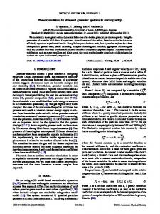
xF i (t), in the same way as in the SDPM. The R-SDPM can be considered as the v0 Q . limit of the SDPM and has the characteristic that long-range correlations are introduced at every time step through this random mixing of the particles. • The second model is the VNM, where the elements are fixed in a 2D lattice. Each set Si (t) consists of exactly K elements which are chosen with probability p within the nearest K neighbors of element i, and with probability 1 − p from anywhere in the system (see Fig. 1). For p=1 every element is connected to its first K neighbors and the network defines a structured 2D topology, as in the XY-model. On the other hand, for p=0 every element is randomly connected to any other K elements of the system, giving rise to a random network topology. It is worth mentioning that for p ] 1 the random selections can be done either at every time-step (annealed dynamics) or only at t=0 (quenched dynamics). As it has been argued in refs. 6 and 8, for connections like the ones considered here (which are established fully at random with any element of the system), the two cases are equivalent. It is worth mentioning that a model similar to our VNM was introduced in ref. 11. Both models introduce a probability of having long-range interactions in an equivalent way, although our system considers a 2D lattice instead of 1D. However, the interactions between spins in the model
Fig. 1. Connectivity of three typical elements in the Vectorial Network Model (VNM). In this model, each element is placed on a vertex of a 2D square lattice (represented by the circles) and connected to K other elements. A fraction p of the K connections are to first neighbors and a fraction 1 − p to any other element in the system. The figure shows the typical linkages of three elements for the case with K=8 and p=7/8.
140
Aldana and Huepe
of ref. 11 are given by the standard XY-model Hamiltonian in the context of equilibrium statistical mechanics. The noise is introduced through the temperature in a Boltzmann distribution and the simulations are carried out by using the Metropolis-Monte Carlo algorithm. In contrast, our VNM is a nonlinear dynamical system in which an additive noise is introduced directly into the interaction rule (1). Note that although the interacting elements are selected at random in both the R-SDPM and the VNM, the randomness is introduced differently in each case. In the latter model, topology imposes no restrictions on the direct random linkages. In contrast, topology does force every element in the R-SDPM to interact with itself (since it is always in its own vicinity) and to interact reciprocally with others (since two interacting particles are always contained in their mutual vicinities). Furthermore, in the VNM the number of elements in each interaction set Si (t) is the same for all i and all t, but in the R-SDPM, Ki (t) is a random variable with mean value OKi (t)P=A(r) r, being A(r) the area of the vicinity of size r and r=N/L 2 the mean density of the system.
3. NUMERICAL RESULTS We will now present some numerical results showing the behavior of the order parameter Y as a function of the noise level g for the models described earlier. Figure 2a displays the bifurcation diagram of Y(g) for the SDPM (crosses) and the R-SDPM (solid line). To generate these curves we started the simulation with all particles oriented in random directions. For each value of g, we run the simulation for a time T long enough for the average in Eq. (2) to reach a steady value. The curves shown in Fig. 2a were computed for systems with N=2 × 10 4 elements in a 2D periodic square box of area L 2=2 × 10 3. For these values of N and L we used an averaging time T=10 5. The vicinity within which other elements interact with any element i was defined as a square of sides r=`15/10, centered at xF i (t). For these values, the average density is r=10 and the mean number of elements in each interaction set is OKi (t)P=15. To describe the dynamics of the SDPM, the values of v0 and Dt also had to be specified since they appear in the kinematic rule (3) which determines the motion of the elements. We used v0 =0.01 and Dt=1. The figure shows the phase transition from the ordered to the disordered regime in the SDPM that has been reported in the literature. (4, 5, 19) Note that this phase transition implying long-range order would be forbidden for an equilibrium system in view of the Mermin–Wagner theorem (13)
Phase Transitions in a Family of Models
141
1 SDPM RSDPM
0.8
(a)
0.6 0.4 0.2 0
Ψ
0
1
2
3
4
5
6
1 VNM, p=0 VNM, P=0.99 RSDPM Analytic solution
0.8
(b)
0.6 0.4 0.2 0
0
1
2
3
4
5
6
η
Fig. 2. (a) Bifurcation diagram for the SDPM (crosses) and the R-SDPM (solid line). The simulations were carried out with N=2 × 10 4 and choosing r and L such that OKi (t)P=15 (see main text). Both models display a continuous second order phase transition from an ordered to a disordered state, in spite of the differences in their underlying dynamics. (b) Bifurcation diagram for the VNM with p=0 (solid line) and p=0.99 (dashed line). The simulations were performed with N=2 × 10 4 and K=15. For comparison, we re-plot the R-SDPM curve shown in (a) (circles). This figure shows that the bifurcation diagrams of the R-SDPM and the VNM are identical. The solid curve in bold is the plot of the analytic solution given in Eq. (17).
since the interactions are local at every moment in time. However, as explained in refs. 15–18, the motion of the elements allows long-range interactions to appear over time since two or more particles which initially were beyond the interaction range r can eventually come together within the same vicinity (see Fig. 3). Figure 2a also shows that an analogous phase transition appears in the R-SDPM, in which the long-range interactions between the particles are forced at every time step via the random repositioning of the particles within the box. It is then apparent that the existence of a phase transition in this family of models does not depend on the specific kinematic rule (3). The above suggests that any other updating rule for the positions that generates long range interactions will also produce a phase transition. Although the SDPM phase transition is analogous to the R-SDPM one, their details differ. In both cases it is a second order phase transition with Y ’ (gc − g) b for |gc − g| ° 1. However, the critical value of the noise gc as well as the critical exponent b are different in the two models. From our numerical results we obtain b=1/2 for the R-SDPM. In contrast, it has been claimed in ref. 4 that b % 0.42 ± 0.03 for the SDPM. Note that this last value of the exponent cannot be read directly from the curve
142
Aldana and Huepe y
x
t
Fig. 3. The motion of the particles in the SDPM produces long-range correlations over time as shown on this diagram. Two particles which at time t=0 are beyond the interaction range can come together within the same vicinity at a later time.
displayed on Fig. 2a. Indeed, although the R-SDPM and SDPM curves were computed for systems with the same number of particles, the higher complexity of the history-dependent SDPM dynamics produces large fluctuations in the instantaneous value of the mean velocity of the system (the integrand in Eq. (2)). This increases the finite size effects, producing a less steep curve in the vicinity of the phase transition. Simulations for bigger systems (N=10 5 ), leading to the value b % 0.42 ± 0.03 for the SDPM, can be found in ref. 4. For completeness, we show our SDPM curve in Fig. 2a which was computed for N=2 × 10 4. The bifurcation diagram for the VNM is shown on Fig. 2b for p=0 and p=0.99. To compare with the results on Fig. 2a, the simulations for the VNM were carried out for systems with N=2 × 10 4 and K=15. We used quenched connections and an averaging time T=10 5. Figure 2b shows that the VNM also exhibits a similar second order phase transition from an ordered to a disordered state when the noise intensity reaches a critical value. Furthermore, the R-SDPM and the p=0 realization of the VNM display identical curves despite the topological differences between them described at the end of Section 2. Note that a phase transition is observed in the VNM even for p=0.99 (only 1% of random connections). However, we know that no transition would occur for p=1 (only local connections), in view of the Mermin–Wagner theorem. 3 This result underlines the critical role of a few long-range interactions in establishing an 3
We checked this point in our numerical simulations, obtaining Y=1 only for g=0 and Y % 0 for g > 0, as expected.
Phase Transitions in a Family of Models
143
ordered phase, in a way that resembles the behavior observed in smallworld networks. (11, 20) 4. ANALYTIC SOLUTION The numerical results presented in the previous section show that the different models within the family that contain a mechanism allowing some degree of long-range interactions exhibit a similar behavior. The R-SDPM and the VNM with 0 [ p < 1 display a phase transition characterized by a critical exponent b=1/2. Furthermore, for p=0 the bifurcation diagrams of the R-SDPM and the VNM become identical. One advantage of the network approach is that it allows us to go beyond the numerical simulations, making an analytical calculation feasible. In this section we will compute analytically the bifurcation diagram near the phase transition for the VNM with p=0. 4.1. The Order Parameter In the limit t Q ., the network reaches a steady state independent of its initial configuration. Assuming that in the steady state all the angles {h1 , h2 ,..., hN } are statistically independent and follow the same probability distribution Ph (a), with a ¥ [ − p, p], we have that the square of the order parameter is given by
7: C Fv : 8 1 75 = lim C cos(h ) 6 +5 C sin(h ) 6 8 Nv 1 = lim F F · · · F 35 C cos(h ) 6 +5 C sin(h ) 6 4 Nv N
1 N 2v 20
Y 2= lim
NQ.
2
i
i=1 N
2 2 0
NQ.
NQ.
2
i
i=1
p
2 2 0
N
2
i
−p
p
−p
i=1
N
p
−p
2
N
2
i
i=1
i
i=1
N
× D [Ph (hi ) dhi ]. i=1
In what follows, without loss of generality, we will set v0 =1. Expanding the square of the sums and using again the statistical independence of the hi ’s we get
5
Y 2= F
p
−p
6 5 2
Ph (a) cos(a) da + F
p
−p
6
2
Ph (a) sin(a) da .
(4)
144
Aldana and Huepe
We thus obtain an expression for the order parameter Y in terms of Ph (a), which is the function that will be used below to describe the state of the system. 4.2. Some Definitions Before computing Ph (a), the stationary distribution function followed by the angles hi , it is convenient to define the following intermediate quantities: • Ph (a; t), the instantaneous probability distribution associated with an arbitrary angle hi (t). In the limit t Q . this function will converge to the stationary distribution Ph (a). FK (t), the vectorial sum of the K vectors in the set Si (t) (the K • V vectors that interact with Fvi (t)): FK (t) — V
C Fv j (t) ¥ Si (t)
Fvj (t).
• PK (a; t), the instantaneous probability distribution of the angle FK (t). The stationary distribution PK (a) is then defined as PK (a)= of V lim t Q . PK (a; t). • Pg (t), the probability distribution of the noise, which is time independent and given by
˛
Pg (t)=
1/g
if t ¥ [ − g/2, g/2],
0
otherwise.
Note that Ph (a; t) and PK (a; t) are defined for any instant in time. In the limit t Q . they transform into their respective stationary probability distributions, Ph (a) and PK (a). 4.3. An Integral Equation for Ph (a; t) From Eq. (1) it follows that Ph (a; t+1) is the convolution of PK (a; t) and Pg (t): 1 g/2 Ph (a; t+1)= F P (a − t; t) dt. g −g/2 K
(5)
Since all the angles {h1 (t), h2 (t),..., hN (t)} are distributed with Ph (a; t), including in particular the ones of the K elements contained in Si (t), it
Phase Transitions in a Family of Models
145
follows that PK (a; t) is entirely determined by Ph (a; t). Equation (5) is therefore an implicit integral equation for Ph (a; t) which can be made explicit by finding how PK (a; t) and Ph (a; t) relate to each other. The resulting relation can then, in principle, be solved for Ph (a; t). In practice, the resulting integral equation is highly involved, and no simple analysis is possible. We will therefore use a different strategy to find Ph (a; t). Since the order parameter given in Eq. (4) is fully determined by the first cosine-sine moments of the stationary distribution Ph (a), we will transform the integral equation (5) into a set of algebraic equations for the instantaneous cosine-sine moments of Ph (a; t) (defined later in Eq. (9)). In the limit t Q . these equations will give the stationary values of the cosine-sine moments that determine the order parameter. 4.4. Computation of PK (a; t) To find how PK (a; t) and Ph (a; t) relate to each other it is useful to FK (t) as make an analogy with a 2D-biased random walk by considering V 4 the total displacement after the K steps Fvj (t) ¥ Si (t). From the geometry shown in Fig. 4 it is easy to see that the joint probability distribution FK (t) satisfies the PK (x, y; t) of the rectangular components (x, y) of V following integral recurrence relation PK (x, y; t)=F
p
−p
PK − 1 (x − cos hiK , y − sin hiK ; t) Ph (hiK ; t) dhiK .
(6)
Taking the two dimensional Fourier transform of the above expression and solving the resulting algebraic recurrence relation, we get
5
ˆ K (l x , l y ; t)= F P
p
−p
6. K
Ph (a; t) e i(lx cos a+ly sin a) da
(7)
Expanding the exponential in powers of l x and l y and bringing the sums outside the integral we obtain
5
.
ˆ K (l x , l y ; t)= C P
n
C
n=0 m=0
i n Dm, n − m (t) m n − m l l m! (n − m)! x y
6, K
(8)
where the instantaneous cosine-sine moments Dm, n (t) are defined as Dm, n (t)=F
p
−p
4
Ph (a; t) cos m(a) sin n(a) da.
(9)
It is a ‘‘biased’’ random walk since the angles hi (t) are distributed according to the nonuniform distribution Ph (a; t).
146
Aldana and Huepe
y
θiK (t) VK (t)
θi3 (t)
α (t) θi2 (t)
θi1 (t) x
FK (t) is the sum of the K vectors contained in Si (t). Therefore, the probFig. 4. The vector V ability distribution PK (a; t) of the angle a(t) can be obtained from the probability distribution FK (t) as the total displacement Ph (a; t) of the angles hi (t). In doing so, it is helpful to visualize V after K steps of a biased random walk, as illustrated above.
We need to perform the inverse Fourier transform of Eq. (8) to obtain PK (x, y; t). In principle, PK (x, y; t) can only be fully determined by the complete hierarchy of moments {Dm, n (t)} . m, n=1 . However, for large values of K, an approximation based on the Central Limit Theorem can be applied by retaining in Eq. (8) only terms up to second order in l x and l y , and identifying this expansion with the one of a bivariate Gaussian funcˆ K (l x , l y ; t) can be expressed as tion. With this approximation P ˆ K (l x , l y ; t)=e iK[D1, 0 (t) lx +D0, 1 (t) ly ] − K2 [s 2c (t) l 2x +s 2s (t) l 2y +2s 2cs (t) lx ly ], P
(10)
where s 2c (t), s 2s (t), and s 2cs (t) are given by s 2c (t)=D2, 0 (t) − [D1, 0 (t)] 2,
(11a)
s 2s (t)=D0, 2 (t) − [D0, 1 (t)] 2,
(11b)
2 cs
s (t)=D1, 1 − D1, 0 D0, 1 .
(11c)
ˆ K (l x , l y ; t) given in The inverse Fourier transform of the approximate P Eq. (10) can now be computed to obtain a bivariate Gaussian distribution
Phase Transitions in a Family of Models
147
for PK (x, y; t). We then find PK (a; t) by transforming (x, y) into the polar coordinates (r, a) and then integrating over r: .
PK (a; t)=F rPK (x(r, a), y(r, a); t) dt. 0
The result is `Dt
e PK (a; t)= 2pAt
−
KCt 2Dt
3 1+B = t
KB
2
5
1 = 2DpKA 264 ,
pK 2Dt At t e 1+Erf Bt 2Dt At
t
t
(12a) where Erf(x) is the error function and At , Bt , Ct , and Dt are defined through At =s 2s (t) cos 2 a+s 2c (t) sin 2 a − 2s 2cs (t) cos a sin a,
(12b)
Bt =[s 2s (t) D1, 0 (t) − s 2cs (t) D0, 1 (t)] cos a +[s 2c (t) D0, 1 (t) − s 2cs (t) D1, 0 (t)] sin a,
(12c)
Ct =s 2s (t) D 21, 0 (t)+s 2c (t) D 20, 1 (t) − 2s 2cs (t) D1, 0 (t) D0, 1 (t),
(12d)
Dt =s 2c (t) s 2s (t) − [s 2cs (t)] 2.
(12e)
4.5. Symmetry of Ph (a; t) and PK (a; t) The symmetry of Ph (a; t) is preserved during the time evolution of the network. Indeed, if at some particular time t we have Ph (a; t)=Ph (−a; t), then at the next time step we will have Ph (a; t+1)=Ph (−a; t+1). The above can be proven as follows. If Ph (a; t)=Ph (−a; t), from definitions (9) and (11) we obtain D0, 1 =D1, 1 =s 2cs =0. Under such conditions, all the odd terms in Eq. (12) disappear resulting in a symmetric PK (a; t). If PK (a; t) is symmetric, then Eq. (5) implies that Ph (a; t+1) will also be symmetric, which in turn implies that PK (a; t+1) is also symmetric, and so on. From the analysis above it follows that, without loss of generality, we can start out the dynamics of the network with a Ph (a; 0) symmetric, thus restricting the evolution to a symmetric PK (a; t) which can be fully determined at every time step by D1, 0 (t) and D2, 0 (t). In this framework, Eqs. (4) and (9) show that the magnetization is simply given by Y=lim t Q . |D1, 0 (t)|.
148
Aldana and Huepe
4.6. Behavior of PK (a) Near the Phase Transition For a symmetric Ph (a; t) we only need to compute D1, 0 (t) and D2, 0 (t). 5 Combining Eqs. (5) and (9) we can establish the following recurrence relation: 1 p g/2 Dn, 0 (t+1)= F F cos n(a) PK (a − t; t) dt da. g −p −g/2
(13)
In the limit t Q . the distribution PK (a; t) will converge to the stationary distribution PK (a) whereas the instantaneous moments D1, 0 (t) and D2, 0 (t) will converge to the stationary values D1, 0 and D2, 0 , respectively. Since PK (a; t) depends explicitly on D1, 0 (t) and D2, 0 (t), in the limit t Q ., the expression (13) transforms into two coupled equations for D1, 0 and D2, 0 . These equations are in general very difficult to solve, but we can find approximate expressions for them which will be valid in the vicinity of the phase transition. It turns out to be that near the phase transition PK (a) can be expressed as PK (a)=P2p (a)+fg (a),
(14)
where P2p (a)=(2p) −1 is a constant probability distribution in the interval a ¥ [ − p, p] and fg (a) is a very small function with the property that lim fg (a)=0
g Q g c−
uniformly.
In order to illustrate this behavior we find numerically the stationary distribution PK (a) for different values of g. This can be done by iterating Eqs. (12) and (13) up to convergence. Figure 5 shows the resulting PK (a) for K=15 and different values of g. In each case the initial probability 2 distribution was Ph (a; 0)=`2/p e −2a . Note that as g approaches the critical value gc % 4.7534 from below, PK (a) uniformly converges to the constant probability distribution P2p (a) for which D1, 0 =0 and D2, 0 =1/2. In fact, from Eqs. (9) and (12) we can deduce that P2p (a) is a trivial ‘‘fixed point’’ 6 of the integral equation (5) for all values of g. The solution Ph (a; t)=P2p (a) corresponds to the case where all elements in the network
5
D0, 2 (t) is also needed, but it is not independent of D2, 0 (t) since they satisfy D2, 0 (t)+D0, 2 (t) =1. 6 P2p (a) is a fixed point of the dynamics in the sense that if Ph (a; t)=P2p (a), it follows from Eqs. (5) and (12) that also Ph (a; t+1)=P2p (a).
Phase Transitions in a Family of Models
149
η=3.50 η=3.90 η=4.30 η=4.70 η=4.72
1
PK(α) 0.5
1/2π 0 3.1416 –π
1.5708 –π/2
0
α
1.5708 π/2
π
Fig. 5. Stationary probability distribution PK (a) for K=15 and different values of g, obtained by iterating Eqs. (12) and (13) up to convergence starting from PK (a; 0)= 2 `2/p e −2a . Note that PK (a) Q P2p (a)=1/2p when g Q gc % 4.7534 from below.
have homogeneous random orientations, for which the order parameter Y vanishes. Since our numerical simulations indicate that the order parameter is always zero for g > gc , we expect Ph (a; t)=P2p (a) to be the only stable solution in this regime. In contrast, for g < gc we have Y ] 0, indicating that the solution Ph (a; t)=P2p (a) becomes unstable and another stable solution appears, as Fig. 5 shows.
4.7. Algebraic Equations for D1, 0 (t) and D 2, 0 (t) Near the Phase Transition In the limit t Q ., Eq. (13) transforms into two coupled algebraic equations for the stationary values D1, 0 and D2, 0 , 1 p g/2 D1, 0 = F F cos(a) PK (a − t) dt da, g −p −g/2
(15a)
1 p g/2 cos 2(a) PK (a − t) dt da, D2, 0 = F F g −p −g/2
(15b)
where PK (a) depends explicitly on D1, 0 and D2, 0 . These equations are in general very difficult to solve because PK (a) is a highly nonlinear function of D1, 0 and D2, 0 . However, the fact that Ph (a) uniformly converges to P2p (a) when g Q gc , allows us to write D1, 0 and D2, 0 around the phase transition as D1, 0 =d,
(16a)
D2, 0 =1/2 − E,
(16b)
150
Aldana and Huepe
with |d| ° 1 and |E| ° 1. Replacing these values into Eq. (12) and expanding PK (a) in powers of d and E up to the third order we get
3
1 PK (a)= 1+`pK cos(a) d − 2 cos(2a) E 2p `pK +(K − 1) cos(2a) d 2+2 cos(4a) E 2+ [cos(a) − 3 cos(3a)] dE 2 `pK (K − 3) + [cos(3a) − cos(a)] d 3 4 − 2[cos(2a)+cos(6a)] E 3+2(K − 1)[cos(2a) − cos(4a)] d 2E
4
3 `pK + [2 cos(a) − 3 cos(3a)+5 cos(5a)] dE 2 . 8 Substituting this result in Eq. (15) and integrating with respect to t and a we obtain the fixed point equations for d and E near the phase transition: `pK sin(g/2) d[4 − (K − 3) d 2+2E+3E 2], d= 4g 1 E= sin g[2E − (K − 1)(1+2E) d 2]. 4g Retaining terms up to d 2 in the solution to these equations, the square of the magnetization Y 2=d 2 as a function of the noise intensity g is finally given by Y 2(g) %
1
2
2(sin g − 2g) g 1− . (K − 2) sin g − (K − 3) g `pK sin(g/2)
(17)
The solid curve in bold on Fig. 2 plots the value of Y(g) as computed from Eq. (17) with K=15. Near gc % 4.7534, the theoretical result and the numerical simulation coincide perfectly as expected. Using Eq. (17) we can find an analytic expression for the critical value of the noise gc by imposing Y(gc )=0. We thus obtain the transcendental equation gc =`pK sin(gc /2).
(18)
The values of K and gc for which this transcendental equation is satisfied are plotted in Fig. 6. Note that gc Q 2p when K Q .. This result has
Phase Transitions in a Family of Models
151
2π 6
ηc
4
2
0
1
10
100
1000
10000
ln K
Fig. 6. Critical value gc of the noise as a function of the connectivity K of the network for the VNM with p=0.
a clear interpretation: when the connectivity K of each element of the network increases, we need to introduce more and more noise to destroy the order generated by the long-range correlations between the elements. It is interesting to note that a very similar behavior occurs in both the SDPM and the simple neural network model introduced in ref. 8. In the SDPM gc approaches 2p when the effective parameter OKP=rr 2 increases, where r is the density of particles and r is the size of the vicinity within which the elements interact (see ref. 19). From the Taylor series expansion of Eq. (17) around gc , it follows that Y 2(g)=C(gc − g)+O((gc − g) 2),
(19)
where C=−
dY 2(g) dg
:
> 0. g=gc
This expansion is valid in the ordered region g < gc . In the disordered region gc < g, Eq. (17) has no real solutions (Y 2 becomes negative). However, in this case Ph (a) is equal to the trivial fixed point P2p (a) and therefore the magnetization vanishes. From the above it follows that the phase transition is described by
˛
Y=
[C(gc − g)] 1/2
for 0 < gc − g ° 1,
0
for g > gc .
(20)
152
Aldana and Huepe
5. CONCLUSIONS In this work we have studied some of the conditions that produce a phase transition in a family of models of interacting 2D elements. By introducing the VNM we have revealed the relevance of the existence of long-range interactions for the emergence of the phase transition in this family of models. A change in the statistical properties of these interactions can vary the nature of the phase transition but cannot eliminate it. For example, the VNM with p ] 1 and the R-SDPM exhibit a phase transition which belongs to the same universality class as the mean field theory (characterized by a critical exponent 1/2). These two models share the property that the long-range interactions between the elements are established in a fully random way. 7 On the other hand, in the SDPM the underlying kinematical rule (3) generates a Markovian process producing long-range interactions which are correlated in time. In this case the phase transition exists but with a critical exponent which seems to differ from 1/2. (4, 5, 19) In contrast, when there are no long-range interactions between the elements, as in the XY-model or the VNM with p=1, the phase transition disappears. Throughout this work we have considered a VNM where each element is connected to exactly K other elements of the system. This assumption can be generalized by considering a model in which the number of connections per element follows a given probability distribution. Work in this direction is in progress. ACKNOWLEDGMENTS We would like to thank Leo Kadanoff and Jennifer Curtis for valuable discussions. This work was supported in part by the MRSEC Program of the NSF under award number 9808595, and by the NSF DMR 0094569. M. Aldana also acknowledges the Santa Fe Institute of Complex Systems for partial support through the David and Lucile Packard Foundation Program in the Study of Robustness. REFERENCES 1. J. J. Binney, N. J. Dowrick, A. J. Fisher, and M. E. J. Newman, The Theory of Critical Phenomena: An Introduction to Renormalization Group (Oxford University Press, Oxford, 1992).
7
This is also true for the simple neural network model analyzed in ref. 8, where binary elements interact through a sort of majority rule plus noise (somehow similar to Eq. (1)).
Phase Transitions in a Family of Models
153
2. P. C. Bressloff, J. D. Cowan, M. Golubitsky, P. J. Thomas, and M. C. Wiener, Geometric visual hallucination, Euclidean symmetry, and the functional architecture of striate cortex, Philos. Trans. Roy. Soc. London Ser. B 356:299 (2000). 3. P. C. Bressloff and J. D. Cowan, An amplitude equation approach to contextual effects in visual cortex, Neural Comput. 14:493 (2002). 4. A. Cziro´k, H. Eugene Stanley, and T. Vicsek, Spontaneous ordered motion of self-propelled particles, J. Phys. A 30:1375 (1997). 5. A. Cziro´k and T. Vicsek, Collective behavior of interacting self-propelled particles, Phys. A 281:17 (2000). 6. B. Derrida and H. Flyvbjerg, Distribution of local magnetizations in random networks of automata, J. Phys. A 20:L1107 (1987). 7. V. S. Dotsenko, Critical phenomena and quenched desorder, Phys. Uspekhi 38:457 (1995). 8. C. Huepe and M. Aldana-González, Dynamical phase transition in a neural network model with noise: An exact solution, J. Stat. Phys. 108:527 (2002). 9. P. C. Hohenberg, Existence of long-range order in one and two dimensions, Phys. Rev. 158:383 (1967). 10. L. P. Kadanoff, W. Götze, D. Hamblen, R. Hecht, E. A. S. Lewis, V. V. Palciauskas, M. Rayl, and J. Swift, Static phenomena near critical points: theory and experiment, Rev. Modern Phys. 39:395 (1967). 11. B. J. Kim, H. Hong, P. Holme, G. S. Jeon, P. Minnhagen, and M. Y. Choi, XY model in small-world networks, Phys. Rev. E. 64:056135 (2001). 12. J. M. Kosterlitz and D. J. Thouless, J. Phys. C 6:1181 (1973). 13. N. D. Mermin and H. Wagner, Absence of ferromagnetism or antiferromagnetism in oneor two-dimensional isotropic heisenberg models, Phys. Rev. Lett. 17:1133 (1966). 14. D. Mukamel, Phase transitions in non-equilibrium systems, in Soft and Fragile Matter: Nonequilibrium Dynamics, Metastability, and Flow, M. E. Cates and M. R. Evans, eds. (Institute of Physics Publishing, Bristol, 2000). 15. J. Toner and Y. Tu, Long-range order in a two-dimensional dynamical XY model: How birds fly together, Phys. Rev. Lett. 75:4326 (1995). 16. J. Toner and Y. Tu, Flocks, herds, and schools: A quantitiative theory of flocking, Phys. Rev. E. 58:4828 (1998). 17. Y. Tu, J. Toner, and M. Ulm, Sound waves and the absence of galilean invariance in flocks, Phys. Rev. Lett. 80:4819 (1998). 18. Y. Tu, Phases and phase transitions in flocking systems, Phys. A 281:30 (2000). 19. T. Vicsek, A. Cziro´k, E. Ben-Jacob, I. Cohen, and O. Shochet, Novel type of phase transition in a system of self-driven particles, Phys. Rev. Lett. 75:1226 (1995). 20. D. J. Watts and S. H. Strogatz. Collective dynamics of ‘‘small-world’’ networks, Nature 393:440 (1998).