Phase transitions in Wilson loop correlator from integrability in global

Phase transitions in Wilson loop correlator

arXiv:1012.1525v1 [hep-th] 7 Dec 2010

from integrability in global AdS.

†

Benjamin A. Burrington and ⋆Leoplodo A. Pando Zayas †

Department of Physics, University of Toronto, Toronto, Ontario, Canada M5S 1A7. ⋆

Michigan Center for Theoretical Physics Randall Laboratory of Physics, The University of Michigan Ann Arbor, MI 48109-1040 Abstract We directly compute Wilson loop/Wilson loop correlators on R×S3 in AdS/CFT by constructing space-like minimal surfaces that connect two spacelike circular contours on the boundary of global AdS that are separated by a space-like interval. We compare these minimal surfaces to the disconnected “double cap” solutions both to regulate the area, and show when the connected/disconnected solution is preferred. We find that for sufficiently large Wilson loops no transition occurs because the Wilson loops cannot be sufficiently separated on the sphere. This may be considered an effect similar to the Hawking-Page transition: the size of the sphere introduces a new scale into the problem, and so one can expect phase transitions to depend on this data. To construct the minimal area solutions, we employ a reduction a la Arutyunov-Russo-Tseytlin (used by them for spinning strings), and rely on the integrability of the reduced set of equations to write explicit results.

1

Introduction

AdS/CFT [1] has become an important tool for studying aspects of strongly coupled gauge theories (for a review, see [2]). In this context, classical minimal area worldsheets have played an interesting role: computing Wilson loop expectation values and quark/anti-quark potentials [3–5]; computing the cusp anomalous dimension [6–8]; computing aspects of large spin or large R-charge operators [9–12]; describing the behavior of string vertex operator correlators for an AdS target space [13–16]; and computing color ordered scattering data [17] using the dual piecewise lightlike Wilson loop. There has been great progress made in this area due to the integrability of the classical worldsheets on AdS (and sphere) backgrounds [11, 12] as well as for the descendent Pohlmeyer reduced theories [18]. These computations often come down to evaluating a regularized worldsheet area and interpreting the exponentiation of this area as being some physical quantity of interest. We first define the Wilson loop operator as a path ordered exponentiation of the gauge field along a closed contour C   Z 1 µ . (1) Aµ dx W [C] = Tr P exp N C The full N = 4 super Yang-Mills (SYM) theory Wilson loop is discussed in [4] and may contain some dependence on the scalar fields as well, however for our discussion we will will set this part to zero. The expectation value of the Wilson loop operator is identified with the appropriately normalized exponentiated classical area of a world sheet ending on the contours C at the boundary of AdS: hW [C]i = exp (−A[C]) .

(2)

Since we have set the scalar part of the Wilson loop operator to zero, we will be studying world sheets that have a profile in the AdS only. The solutions we will discuss are therefore applicable in any theory with an AdS factor in the geometry, however, one may need to be careful about the gs corrections to these backgrounds, as we shall discuss in a moment. In what follows, we will be concerned with two Wilson loop operators, defined by two circular contours. A natural object to study is [5, 19], X λ2n hW [C1 ]W [C2 ]i =1+ fn (λ, C1 , C2 ). hW [C1 ]ihW [C2 ]i N 2n n

(3)

These have been previously studied for Minkowski space holographically in [19–22], and see [23] for a field theory discussion. One can argue for the above expansion 1

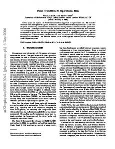
simply using large N arguments. The first two terms, 1 and N12 , are in some sense planar terms, where the 1 is enhanced due to being a “disconnected” diagram, and the order N12 term comes from connected planar diagrams. Higher order terms come from non-planar diagrams. Further, we have extracted a certain power of λ to make this look like a gs expansion, but is otherwise artificial, and could be absorbed into the definition of fn . In the string picture, we expect to compute a set of diagrams given in figure 1. The fact that we want to compute a ratio of the form (3) means that we want to

(gs)

0

+

+

+ ......

(gs) 2

(gs) 4

Figure 1: A diagramatic expansion of the worldsheets living in AdS. We have normalized the first term to be order one ((gs )0 ), so that the subsequent labels correspond to the degree to which they are sub-leading. regulate all of the areas of the above worldsheets by subtracting off the area of the disconnected leading order piece, i.e. to compute X 
 hW [C1]W [C2 ]i = 1+ gs2n exp − Anconnected [C1 , C2 ] − A0disconnected [C1 , C2 ] (4) hW [C1]ihW [C2 ]i n where Anconnected is the connected diagram with Euler character −2n + 2. The disconnected part is actually two distinct parts, coming from the area of the two disconnected pieces. We recognize this expansion as being the same as the previous 2 expansion because gs = gYM = Nλ , and the exponentiated area plays the role of the function fn . Here we have relied on the S5 in the AdS5 ×S5 geometry in a subtle way: we have assumed that the background has no gs corrections. Hence, for more general setups, like Sasaki-Einstein or orbifold backgrounds, more care may be needed; see [24] for recent work in this direction. In such cases, there is a second type of gs correction coming from the corrected worldsheet action due to the gs correction to the background. Therefore, lower genus diagrams will contribute to a given order in gs . For us, we will be discussing f1 , and so this correction would amount to evaluating the old double cap solution in the correction to the sigma model action. 2

In fact, because we divide by a pair of hW i expectation values, we expect that this correction is in fact divided out and so we expect that the above is sufficient for leading N12 order corrections in any background with an AdS. However, for higher corrections, one would need to be more careful, and check the contributions of lower genus worldsheets in the corrected action, as well as needing to modify the equations one solves. The purpose of this paper is to compute the first correction term in the above expansion in global AdS coordinates, namely, that associated with the “diagram” in figure 2. We compute this analytically for two synchronous coaxial same-size

− Figure 2: A diagramatic expansion of the first non trivial term we will compute. This gives the function f1 at strong coupling. spacelike Wilson loops, separated by an interval in one of the angular coordinates (φ) of the S3 inside of AdS5 , and we find ln(f1 ) = − (Aconnect − Acap×2 )   √   1 2 = − 4πλ 1 − √ (5) −(1 − k )K(k) + E(k) 2k 2 − 1

with k defined through the following relation  2   √  2k − 1 2k 1 − k 2 1 − k2 Π ,k exp √ K(k) − k2 k2 2k 2 − 1 q

cos(θ0 ) sin2 (θ0 ) + tan2 ∆φ + tan ∆φ 2 2 = q

tan ∆φ cos(θ0 ) − sin2 (θ0 ) + tan2 ∆φ 2 2

(6)

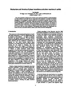
and where θ0 defines the “radius” of the two Wilson lines, and ∆φ determines the distance between their center points (see fig. 3). The functions K and Π (and E later on) are complete elliptic integrals, see appendix B. The above is valid for k < kc where this critical value is given by !   1 −(1 − kc2 )K(kc ) + E(kc ) = 0 (7) 1− p 2 2kc − 1 3

ψ C2

∆φ

C1

S3

θ0

ψ

Cartesian Limit ∆φ 0, θ0 0 ∆x

R3

R

Figure 3: Here we diagram the boundary conditions specifying the two equal size contours we use to explicitly calculate the Gross-Ooguri transition. The Cartesian limit gives the flat space behavior. which is numerically found to be kc = 0.8232.

(8)

Using this value of kc , one finds that the Gross-Ooguri transition happens at a ∆φ defined by   sin2 (θ0 ) ∆φc 2 (9) = (E+1)2 tan 2 2 2 cos (θ0 ) − 1 (E−1)

where E ≈ 2.4034 1 . For ∆φ exceeding this value, the disconnected graph is preferred, and the transition is found to be first order, as in the flat Minkowski space case [19]. The flat Minkowski space limit is easy to read off, taking a θ0 → 0 limit, this reads ∆xc = 0.9052R agreeing with the result given in [19]. We also find that for sufficiently large Wilson loops that the connected solution always dominates, due to the finite separation distance possible on the sphere. This critical size is given approximately by (E − 1)2 (E + 1)2 ≈ 0.3547π.

sin2 (θcrit ) = 1 − θcrit

(10)

We see no problem with extending this to non-synchronous and non-equal-size Wilson loops, given the structure of the equations we find in the subsequent sections, 1

E is just the value of exp



√ 2 2k √ 1−k 2k2 −1



K(k) −

1−k2 k2 Π

4



2k2 −1 k2 , k



evaluated at k = kc .

although the above mentioned situation is the most symmetric. We comment on the structure of these more general surfaces in the text and in the appendix. One final note is in order. When the disconnected configuration is preferred, we expect that the correct N12 correction is given by the disconnected area (i.e. 1, given that we have divided by this) times a propagation of a bulk field between the two disconnected caps: this is outside the scope of our current work, and has already been addressed in [5] for Minkowski space (for similar work for the null polygonal Wilson loops, see [25]). We organize the paper as follows. In section 2 we compute the equations of motion for the minimal surface in AdSn , and write the two dimensional (2D) Lax pair associated with this system. We reduce this Lax pair as in [11] and find a reduced one dimensional (1D) Lax pair. This furnishes a set of 1D first order equations of motion, which we separate, and show how to solve by iterative integration. In section 3 we write down several explicit solutions, including that for the synchronous coaxial Wilson loops, and synchronous coaxial equal-sized Wilson loops. We compute the regulated area minus the regulated area of the disconnected worldsheet to find the function f1 above, and compute the Gross-Ooguri transition point, and the critical radius where the transition no longer occurs. In section 4 we discuss possible future work.

2 2.1

Equations of motion, reduction to 1D system. Equations of motion, and reduction

We first obtain the equations of motion for a string in AdSn . Recall that AdSn is given by the restriction
2
2
2
2 − Y −1 − Y 0 + Y 1 · · · + Y n−1 = −1 (11) in R2,n−1. We will avoid using the flat space R2,n−1 metric for computing the scalar product, and simply write “·”. We implement the above restriction via a Lagrange multiplier Ξ in the Polyakov action, giving Z
¯ − Ξ (Y · Y + 1) . S = dzd¯ z ∂Y · ∂Y (12)

Upon elimination of Ξ, the equations of motion read

¯ M = (∂Y · ∂Y ¯ )Y M ∂ ∂Y Y · Y = −1 5

(13)

and further, we have the Virasoro constraint ¯ · ∂Y ¯ = 0. ∂Y · ∂Y = ∂Y

(14)

One may take the above (13) and antisymmetrize in a Y N to find ¯ M ] = 0. Y [N ∂ ∂Y

(15)

This is in fact invertible, one may obtain (13) from (15) by dotting in a Y N , and using Y · Y = −1. Finally, we rewrite the above as

¯ M ] + ∂¯ Y [N ∂Y M ] = 0 ∂ Y [N ∂Y (16)

to write the above as a total divergence. We can repackage these equations into equations of motion resulting from a Lax pair formulation, which we turn to now. First, writing the fields in some matrix g (which we explicitly show below), and ¯ −1, the equations of motion can be obtained via the defining A = ∂gg −1 , A¯ = ∂gg Lax pair with spectral parameter λ     A¯ A ¯ Ψ = 0, Ψ = 0. (17) ∂− ∂− 1+λ 1−λ The integrability condition for the two equations is  ¯ − (1 + λ)∂ A¯ + [A, A] ¯ (1 − λ)∂A − Ψ = 0. (1 + λ)(1 − λ)

(18)

which in the current context implies both the equation of motion (see footnote 2)

and gives the identity

¯ + ∂ A¯ = 0 ∂A

(19)

¯ − ∂ A¯ + [A, A] ¯ = 0. ∂A

(20)

In the above A, A¯ plays the role of a gauge connection, and so we see that (17) is invariant under Ψ = χΨ′ A = χA′ χ−1 + (1 + λ)∂χχ−1 ¯ −1 . A¯ = χA¯′ χ−1 + (1 − λ)∂χχ 6

(21)

Usually, we allow for any transformation χ(z, z¯, λ) such that A′ and A¯′ are again independent of λ. However here, our concerns will be more general and so below we will allow for any χ. Next, we wish to write these equations in Cartesian components, and for this, we ¯ ∂τ = 1 i(∂ − ∂). ¯ Therefore, in these coordinates, we find recall that ∂σ = 21 (∂ + ∂), 2 the Lax pair       1 A 1 A A¯ A¯ ∂σ − Ψ = 0, ∂τ − i Ψ = 0. (22) + − 2 1+λ 1−λ 2 1+λ 1−λ which can be written    Aσ + iλAτ ∂σ − Ψ = 0, 1 − λ2

   Aτ − iλAσ ∂τ − Ψ = 0, 1 − λ2

(23)

where Aσ = ∂σ gg −1, Aτ = ∂τ gg −1. The gauge transformations can be read from the last ones quite easily and give Ψ = χΨ′ Aσ = χA′σ χ−1 + ∂σ χχ−1 − iλ∂τ χχ−1 Aτ = χA′τ χ−1 + ∂τ χχ−1 + iλ∂σ χχ−1 . (24)
+iλAτ We define the combination Aσ1−λ = Vσ and similarly for Vτ . We will wish to 2 reduce this model on a circle for a particular Ansatz, and we turn to this now. A particular choice of g for AdS5 is given by 2   0 Z1 −Z3 Z¯2 −Z1 0 Z2 Z¯3   (25) g=  Z3 −Z2 0 −Z¯1  −Z¯2 −Z¯3 Z¯1 0 where we have defined

√ Z1 = Y −1 + iY 0 = eit 1 + r 2 , Z2 = Y 1 + iY 2 = eiφ cos(θ)r, Z3 = Y 3 + iY 4 = eiψ sin(θ)r.

(26)

Here we could have used the choice g = Y · Γ where ΓI are the SO(2, n − 1) (n=5) gamma matrices. This is particularly easy because ∂gg −1 = ∂YI YJ ΓIJ , and likewise for the ∂¯ part of the connection. This makes the equation (19) read exactly as (16), so this is indeed the equations of motion. Here, to reduce the size of the matrices we are working with the 4 × 4 chiral components of the SO(2, 4) matrices, which are a constant similarity transformation away from the g given here. 2

7

This gives a particular parametrization of the homogeneous coordinates Y I that solves the quadratic constraint (11). For this choice, the metric appears as ds2 = ηIJ dY I dY J = −(1 + r 2 )dt2 +


dr 2 + r 2 dθ2 + cos2 (θ)dφ2 + sin2 (θ)dψ 2 2 (1 + r )

(27)

We wish to make a reduction along a circle, and take that the σ direction is compact, and we want to consider the solutions given by ψ(σ, τ ) = wσ

(28)

and all other functions are functions of y only. Now, we ask the question of whether there exists some connection Vσ that is σ independent after a gauge transformation. Indeed we find that there is one, and it is given by  i  e− 2 wσ 0 0 0 i   e 2 wσ 0 0   0 χ= (29) . i  0 0  0 e− 2 wσ i 0 0 0 e 2 wσ

In fact, this makes both Aσ and Aτ independent of σ altogether. One may be concerned that the functions above are not well defined on the circle (e.g. w an odd integer it is not well defined). However, going around the circle in σ either takes χ to itself or χ to minus itself, but in the gauge transformation, χ only appears “squared” so that the resultant connection is well defined. The new connections Aσ and Aτ depend on λ in some new way, however. Now we note that this simplifies our lives quite a bit. The Lax equations now read ∂τ Vσ − ∂σ Vτ + [Vσ , Vτ ] = 0

(30)

however, Vτ is σ independent, and so we find ∂τ Vσ = [Vτ , Vσ ]

(31)

which can be thought of as the one dimensional Lax pair L′ = [M, L]

(32)

where ′ is now τ differentiation. In such a formulation, the conserved quantities are given by Tr (Ln ) because ∂τ Tr (Ln ) = nTr (L′ Ln−1 ) = nTr ([M, L]Ln−1 ) = 0 by the 8

cyclicity of the trace. Since L is still a rational function of λ, we expect there to be only a finite number of conserved quantities of this form. The above discussion is in fact the same reduction as was found in [11]: here we are using a subclass of Ansatz setting certain winding numbers to zero, and setting some dynamical functions to zero. However, here we will be considering the most general solutions to the system that we have found, rather than focusing on “constant radii” solutions discussed in [11]. In fact, the above Lax pair is insufficient to furnish all conserved quantities. However, it does furnish one that is not so obvious. To obtain a Lax pair furnishing all conserved quantities, one may simply redefine L + I(Pt + λPφ ) where I is the identity matrix, and Pt and Pφ are conserved quantities that we can find some other way3 . This will not be needed for our further discussion, and we simply state a set of conserved quantities Pt = (1 + r 2 )t′ Pφ = r 2 cos2 (θ)φ′
(r ′ )2 + r 2 (θ′ )2 + cos2 (θ)(φ′ )2 − w 2 sin2 (θ) (33) 2 1+r (r ′ )2 sin2 (θ) + 2 sin(θ) cos(θ)rθ′ r ′ H2 = sin2 (θ)(1 + r 2 )r 2 (t′ )2 + 2 1 + r

+ cos2 (θ) − r 2 sin2 (θ) r 2 (θ′ )2 + r 2 − sin2 (θ) cos2 (θ)r 2 (φ′ )2 − w 2 sin2 (θ) . H1 = −(1 + r 2 )(t′ )2 +

Note that H1 is just the the hamiltonian resulting from the reduced action. Further, it must be 0 for the above system to correspond to a minimal surface: H1 = 0 is the Virasoro constraint. Next, we will eliminate t and φ from the discussion by replacing them with the conserved quantities Pt and Pφ . Doing so, we find   Pφ2 (r ′ )2 Pt2 ′ 2 2 2 2 + + r (θ ) + 4 − w sin (θ) (34) H1 = − 1 + r2 1 + r2 r cos2 (θ) P 2 r 2 sin2 (θ) (r ′ )2 sin2 (θ) H2 = t + + 2 sin(θ) cos(θ)rθ′ r ′ 1 + r2 1 + r2 ! 2 2
P sin (θ) φ − w 2 sin2 (θ) . (35) + cos2 (θ) − r 2 sin2 (θ) r 2 (θ′ )2 + r 2 − 2 r cos2 (θ) The above quantities are conserved simply using the reduced equations of motion. However, since we are looking for a particular class of solutions, H1 = 0, we will find 3

Perhaps there is a more “efficient” Lax pair than the one we find here

9

other linear combinations more useful. We take instead the combinations 2

(− cos(θ)r ′ + sin(θ)r(1 + r 2 )θ′ ) 1 + r2 (1 + r 2 sin2 (θ))((1 + r 2 )Pφ2 − Pt2 r 2 cos2 (θ)) − r 2 (1 + r 2 ) cos2 (θ)

H1 = (H2 − H1 ) = −

H2 = (H2 + r 2 sin2 (θ)H1 ) = (sin(θ)r ′ + r cos(θ)θ′ )
−w 2 r 2 sin2 (θ) 1 + r 2 sin2 (θ)

(36)

2

(37)

where now the Virasoro constraint reads H1 = H2 ≡ H. Note that H2 is only conserved quantities when the Virasoro constraint is met. Further note that the above combinations are special in that the single derivative term squared can be written as a total derivative. This allows us to write the above differential equations as   r cos(θ) ∂τ √ = 1 + r2 v u  2 r cos(θ) 1 u 1 2 2 2 u −H + Pφ + Pt − Pt √ ± (38) − Pφ2  2 t 2 1+r r cos(θ) 1 + r2 √ 1+r 2

p ∂τ (r sin(θ)) = ± w 2 (r sin(θ))4 + w 2 (r sin(θ))2 + H.

(39)

The second equation can be solve directly by integrating (note the right hand side is a function of r sin(θ) only). Let us denote r cos(θ) , F1 = √ 1 + r2

F2 = r sin(θ),

(40)

so that the above equations may be written

F1′ = ±

1 − F12 1 + F22

s

q F2′ = ± w 2 F24 + w 2 F22 + H

−H + Pφ2 + Pt2 − Pt2F12 − Pφ2

1 . F12

(41) (42)

Along with the equations 1 − F12 1 + F22 1 − F12 ′ φ = Pφ 2 F1 (1 + F22 ) t′ = Pt

10

(43) (44)

give all of the equations of motion. Therefore, one solves (41) for F2 , then using this result, solves (42). This is possible because the right hand side of (42) is a function of F1 times a function of F2 : since F2 is a known function of τ , one can integrate this with respect to τ and integrate with respect to F1 on the left, furnishing F1 as a function of τ . With F1 and F2 in hand, one may then directly integrates (43) and (44) find the general result. There is an important simplification here. R dτ When integrating the F1 equation, (42), one will be forced to do the integral 1+F 2 , and 2

dτ then F1 will be written as a function of this variable. However, this measure 1+F 2 2 will appear when integrating to find t and φ as well. Therefore, one can change to the coordinates defined by this integration measure, and simplify the integration. We will use this trick later, and emphasize it again when we turn to computing the solutions. Finally, if one wishes, one can solve the equations for non zero H1 , and this only changes the coefficient of F22 in (41), and the value of H appearing in (42), and so does not affect the method of solving the equations, nor the form of the equations. When considering profiles on the S5 part of the geometry this will become important, but does not appear to be a major obstacle, given these simple modifications (see [26] for example). We now segue a bit and discuss the sections of F1 and F2 that are allowed. First, r is a positive definite number, and so the signs of F1 and F2 are actually given by θ. Recall that for one cover of the S3 inside of AdS5 we have that 0 ≤ θ ≤ π2 to get a single covering. Extending θ beyond this bound is relatively straightforward, as passing through θ = 0 can be compensated for by (−θ, φ, ψ) → (θ, φ, −ψ), as these define the same homogeneous coordinates (and is the usual way for going through
such an “origin”). Similarly, for going through θ = π2 we see that π2 + θ, φ, ψ →
π − θ, −φ, ψ . We can, therefore, make sense out of all signs for F1 and F2 . However, 2 < 1. Hence, any solution that we find for F1 must lie in note that −1 < F1 = r√cos(θ) 1+r 2 this range. Another way of saying this is that   1 + F22 F22 1 − F12 2 2 r = − 1 , tan (θ) = . (45) 1 − F12 F12 1 + F22

One should note that these expression define a real r and a real θ for any real F1 , F2 that satisfy F12 ≤ 1, and no restrictions on F2 . There is one final note. Given the Virasoro constraint, one can get the pullback metric immediately as
ds2 = w 2 F22 dτ 2 + dσ 2 (46) 11

allowing direct computation of the lagrangian density as Z L2 w 2 dτ dσF22 S= ′ 4πα

(47)

where we have reintroduced the AdS radius L. The above should be read with some care, however, when talking about Euclidean worldsheets: these require an extra factor of i. This will render our exponentiated action as being exponential suppression, and so should be understood as a tunneling event: we have already accounted for this in equation (2), where the area is to be read as the classical Euclidean area of the worldsheet. This exponential suppression is not surprising because we will be considering space-like separated 4 space-like Wilson loops.

3

Solutions

3.1

Special case: H = 0

Let us work out a simpler set of equations as a warm up. We take H = 0 above, and take ± = + for the F1 equation and ± = − for the F2 equation, and find 1 sinh(w(τ − τ0 )) v u 2 u (Pt − Pφ2 )2 C2 + (τ − τ0 ) − F1 (τ ) = t (Pt2 − Pφ2 )2 C2 + (τ − τ0 ) −

(48)

F2 (τ ) =

1 w 1 w

tanh(w(τ − τ0 )) tanh(w(τ − τ0 ))


2
2

+ Pφ2 + Pt2

.

(49)

Note that this F1 and F2 define a good θ and r given the restrictions mentioned above, and further, the signs were chosen so that 0 ≤ θ ≤ π2 . Particularly, F12 < 1 is always true as long as Pt2 > Pφ2 , i.e. that |Pt | > |Pφ |. Given the above functions, one can integrate the expressions for t(τ ) and φ(τ ) and further, one may rearrange the above expressions to solve for r(τ ) and θ(τ ). 4

All points of each Wilson loop are space-like separated from all points of the other Wilson loop

12

Upon doing so, we find v   2 u 1 u cosh2 (w(τ − τ0 )) (Pt2 − P 2 )g0 (τ )2 + 2Pφ 2 + φ t Pt −Pφ cosh2 (w(τ −τ0 )) r(τ ) = sinh2 (w(τ − τ0 )) s ! Pt2 − Pφ2
θ(τ ) = arctan cosh2 (w(τ − τ0 )) (Pt2 − Pφ2 )2 g0 (τ )2 + Pφ2  2  (Pt − Pφ2)g0 (τ ) t(τ ) = arctan + t0 Pt   2 (Pt − Pφ2 )g0 (τ ) + φ0 φ(τ ) = arctan Pφ

(50) (51) (52) (53)

where we have defined the useful functions g0 (τ ) = C2 + (τ − τ0 ) −

1 tanh(w(τ − τ0 )). w

(54)

Note that in the above, we have the following constants of motions Pt , Pφ , C2 , t0 , φ0 , τ0 , and we have 4 dynamical fields. In general, we would expect 8 constants of motion for these equations, however, we must take H1 = 0 to describe minimal surfaces, and we have taken the slice H = 0 as well, hence we are left with six constants describing the surface. Finally, note that in the limit τ → 0 that the surface goes to a circle, and τ → ∞ it goes to a point. This may have some bearing on the calculations performed in [27], however, we do not regulate these areas, and so we will have little to say on this point here. 3.1.1

Sub-sub case: the single cap solution.

We now explore a particular solution with F1 = const, H = 0, w = 1, Pt = Pφ = 0 that will be important for later. Note that in the above discussion, plugging in H = 0, one can take a limit with F12 → Pφ2 /Pt2 being a fixed ratio less than one, but still get Pφ = Pt = 0. In this limit, the solution reduces to 1 sinh τ F1 = F0 ≡ cos(θ0 ) t = t0 φ = φ0 . F2 =

13

(55)

where we have taken w = 1 for a single winding. For multiple windings, one can simply take τ → wτ in the above equation. This “single cap” solution is well known [4, 5] This gives a particularly simple solution 2

r =

cos2 (θ0 ) +

1 sinh2 (τ )

sin2 (θ0 )   tan(θ0 ) θ = arctan . cosh(τ )

(56) (57)

This solution is the “single cap” solution. This is easiest to see in the following way. First, note that when τ → 0, the radius goes to infinity, and theta goes to some value fixed by θ0 . Therefore, the constant sin(θ0 ) determines the radius of the Wilson loop. Then, when τ → ∞ we see that θ → 0 and r → const, where again this constant is determined by θ0 . However, we note that the pullback metric (46) gives ds2 =


1 dτ 2 + dσ 2 . 2 sinh (τ )

(58)

We would like to determine what the nature of the “cutoff” is when τ → ∞. It is easy to see that in this limit, the pullback metric (46) reduces to
ds2 = e−2τ dτ 2 + dσ 2 , (59) and changing variables to T = e−τ , we see that the metric becomes
ds2 = dT 2 + T 2 dσ 2 ,

(60)

where now the above limit is T → 0. Because the periodicity of σ is 2π, this represents a smooth point of the worldsheet, and is just a place where the round “cap” surface pinches off to zero size in a smooth way. If we had instead left w to be an integer winding number, the asymptotic form of the metric would have become
ds2 = w 2 e−2wτ dτ 2 + dσ 2 (61) which can be transformed by the coordinate transformation T = e−wτ ds2 = dT + w 2 T 2 dσ 2 .

(62)

This gives a conical singularity at the point T = 0, with an excess of angular “space” given by w. This, of course, is easy to visualize: the multiple windings are collapsing to a point, giving multiple covers of the flat space metric. 14

3.2

Finding F2 for general conserved quantities.

Now let us look to the general H 6= 0 case. We write this as ! ! F22 F22 ′ 2 2 4 2 2 √ √ 1− (F2 ) = (w F2 + w F2 + H) = H 1 − − 12 + 1−γ − 12 − 1−γ 2 2

(63)

where

4H . (64) w2 We recognize the above differential equation as being solve by Jacobi elliptic functions, however, it is not immediately clear how to write them in a manifestly real way. However, it is clear is to break the discussion √ into cases where certain reality conditions are met. We note that the combination 1 − γ is either real or imaginary depending on whether γ is larger or smaller than 1 (w is assumed to be real). Hence, γ = 1 is a special value (in fact, this makes the right hand side of the equation above a perfect square,√ and this can be solved nicely too). However, there is also a crossover when − 21 + 1−γ is positive or negative, in other words when γ = 0 (this 2 is the case H = 0 above). Hence we wish to break the problem into three cases: γ=

1. γ < 0 (H < 0) 2. 0 < γ < 1 (0 < H < w 2 /4) 3. γ > 1 (H > w 2 /4). After a bit of work, and using various identities following solutions for these cases     √√ 1 1 1−γ+1  dn 1  , (1 − γ) 4 sn w(1 − γ) 4 τ, √2  1  (1−γ) 4      q √ 1 √ √ γ 2(1−γ) 4 1−γ cn wτ 1 q √ + , √ ±F2 = √ 2 2 sn 2 1 1+ 1−γ  − 1−γ 2 2    √  √ 1  γ−1  4 cn  √wτ √ , √ 1  γ√2 sn·dn 2 γ 2γ 4

[28–30], we can arrive at the

if γ < 0, (H < 0) if 0 < γ < 1, (0 < H < if γ > 1, (H >

w2 ) 4

w2 ) 4

(65) where the relative “phases” associated with shifting τ → τ − τ0 have been chosen so that the terms agree on the boundary of their relative regimes (γ = 0, 1). Above we have used a condensed notation where it is understood that all elliptic function have the same arguments, for example h cn i cn(z, k) (z, k) ≡ . (66) sn · dn sn(z, k)dn(z, k) 15

10

5

F

0

2

K

5

K

10 0

1

2

at

3

4

5

Figure 4: Here we have plotted F2 (τ ) for one connected component of the worldsheet (where the arguments of the elliptic functions range between 0 and 2K(k) for the appropriate k). The graphs depict different values of γ = [−5, −2, −0.3, 0, 0.5, 2, 6] corresponding to the colors (line styles) [red (dot), orange (dash), brown (dash-dot), black (solid), dark green (wide space dot), blue (long dash), violet (wide spaced dash)]. Also note that in the above, the modulus (usually denoted “k”) of all functions is less than one. This gives some nice results. First, because 0 < k < 1 we have that dn is positive definite, and both cn and sn are functions with amplitude 1. Thus, dn 1 is a generalization of a “ sin ” function. We can see this by remembering that all sn elliptic function have period 4K(k) where K(k) is the complete elliptic function, and that sn(0, k) = 0 and sn(2K(k), k) = 0: it goes to zero at 0 and at the period over 1 cn 2. This then will have exactly the same shape as sin . Similarly, cn and sn·dn are in sn some sense generalizations of cot (blowing up at 0 and period over 2, but crossing the horizontal τ axis). This gives a rough idea of how these functions behave. We plot them to emphasize the point in figure 4. We note that in these graphs where H > 0 that the worldsheet has been reflected through the origin: it has shrunk to zero size and then reemerged to finite size. We take that this is an orientation reversal of the world sheet. and this corresponds to reversing the orientation of the second Wilson loop operator. Hence, later when we define “coaxial” we will mean “coaxial with the same orientation.” Reversing the orientation of one Wilson loop is considering the complex conjugate of the original Wilson loop operator, and we expect the correlator to depend on this information. We will not consider correlators of this form, “hW [C]W [C]† i”, and leave this to 16

future work.

3.3

Synchronous coaxial Wilson loops, and the Gross Ooguri phase transition.

We now turn to looking at a special class of solutions given a pair of Wilson loop operators that are synchronous, spacelike separated, and with the same orientation. Given these conditions and the above discussion, we see that this is a case where Pt = 0, but Pφ 6= 0 and H < 0 (see also appendix A). In this case, the equations of motion simplify, and rather than arctan functions for the F1 integral, as in appendix A, we get instead logs. Solving these equations becomes relatively straightforward, as one simply needs to integrate to find F1 , and we find " !# p√ 1 1 1 4H dn 1−γ+1 , γ= 2 0 (75) 1 (1 − γ) 4 and one takes the positive square root to determine F1 . We have included an “integration constant” C2 here, associated with the fact that we have defined I1 by a definite integral. This F1 lies in the acceptable range 0 < F12 < 1. This can be seen by noting that the numerator and denominator are both positive definite (given 19

that H < 0), and noting that the numerator minus the denominator is sign definite, given the sign of C2 , and requires C2 > 0 so that it is negative. This restriction on C2 is quite natural because it comes about as the exponentiation of an integration constant: if this constant is real, C2 > 0. Finally, because F2 is real, these functions define a real r and θ. The final integrationR for φ can be explicitly performed. This is because F1 is a dτ dτ function of the variable 1+F 2 . The φ integral actually has this factor 1+F 2 built in, 2 2 and so we integrate this directly, obtaining6  √    −γ 4 2 C exp I + 4P + 4P H 1 1 φ φ  2  (1−γ) 4 . √ φ = φ0 − arctan  (76)   8Pφ3 −H So far, our discussion has been for general radius Wilson loops. In fact, one can see immediately that since F1 is in the appropriate range, and because I1 has no singularities at finite τ , that F1 goes to constant values when F2 diverges. This gives that the endpoints of 0 < τ < 2K(k) 1 are at the boundary of AdS (this is the only w(1−γ) 4

way to get a divergent F2 and finite F1 ). In fact, at these endpoints, C2 helps fix the size of the two Wilson loops. Next, we note that the function I1 is monotonically increasing increasing τ : R for dτ this is easy to understand because it is related to the integral 1+F 2 which has a 2 positive definite integrand. Therefore we see that there is no way for the function   g = C2 exp

√

−γ

1

(1−γ) 4

I1

to be constant unless C2 = 0, but this case is F1 = 1 which

is forced to be on the boundary the entire time with θ = 0 fixed. However, we may ask the questionof when F1 has  the same value at the two endpoints, namely when F1 (τ = 0) = F1 τ =

K(k)

1

w(1−γ) 4

: this is where the two Wilson loops have the same

6 note that if we had let Pt 6= 0 that the t equation of motion shares this property, so in the general case, both of these equations may be integrated using this variable to eliminate F2 in a straightforward way.

20

size. This occurs when  2   √ −γ 4 2 + 4Pφ + 4Pφ H − 64Pφ6H C2 exp 1 I1 (0) (1−γ) 4   √ 2  −γ 2 4 C2 exp + 4Pφ − 4Pφ H 1 I1 (0) (1−γ) 4    √  2 K(k) −γ 4 2 C2 exp + 4Pφ + 4Pφ H − 64Pφ6 H 1 I1 1 (1−γ) 4 w(1−γ) 4 − = 0.   √  2  −γ K(k) C2 exp + 4Pφ4 − 4Pφ2H 1 I1 1 (1−γ) 4

(77)

w(1−γ) 4

This happens when either C2 exp

√

−γ

1

(1 − γ) 4

I1 (0)

!

= C2 exp

√

−γ

1

(1 − γ) 4

I1

K(k) 1

w(1 − γ) 4

!!

(78)

which, again, due to I1 being monotonic, cannot happen unless C2 = 0; or they are equal when !
2 √ 16Pφ4 Pφ2 − H −γ  √   . C2 exp = (79) 1 I1 (0) (1 − γ) 4 −γ K(k) C2 exp 1 I1 1 (1−γ) 4

w(1−γ) 4

We have normalized so that I1 (0) = 0 and so we get
4Pφ2 Pφ2 − H  √   . C2 = −γ K(k) exp 1 I1 1 2(1−γ) 4

(80)

w(1−γ) 4



√

−γ



with This value of C2 is special. It essentially dresses the factor of exp 1 I1 (τ ) (1−γ) 4
a factor 4Pφ2 Pφ2 − H and re-zeros the function I1 such that it is odd via reflection about τ = K(k) 1 . This, in fact, renders the function F1 even with respect to this w(1−γ) 4

reflection. Therefore, the solution connecting two synchronous coaxial equal radius Wilson

21

loops is 

 dn F2 (τ ) = (1 − γ) (z, k) sn  2   √ −γ 4 2 + 4Pφ + 4Pφ H − 64Pφ6H C2 exp 1 I1 4 (1−γ) F1 (τ )2 =   √  2 −γ C2 exp + 4Pφ4 − 4Pφ2H 1 I1 (1−γ) 4   √   −γ 4 2  C2 exp (1−γ) 14 I1 + 4Pφ + 4Pφ H  . √ φ = φ0 − arctan    8Pφ3 −H 1 4


4Pφ2 Pφ2 − H  √   C2 = K(k) −γ exp 1 I1 1 2(1−γ) 4 w(1−γ) 4 "   2k 2 − 1 (1 − k 2 ) Π sn(z − K(k), k), , k Θ(sn(z, k)) I1 (τ ) ≡ z − k2 k2   2 #  (1 − k 2 )Π 1, 2kk2−1 , k  i  z z + . − ln eiπ( K(k) −1) − k2 π K(k) q√ 1−γ + 12 4H 1 2 γ = 2 < 0. k= , z = w(1 − γ) 4 τ, 1 w (1 − γ) 4

(81)

Due to the choice of C2 one can readily check that F1 is symmetric with reflection about τ = K(k) 1 , and further, so is F2 . Finally, one can also see that the function w(1−γ)   4 K(k) + const, and so the entire surface is symmetric φ(τ, Pφ ) = φ 1 − τ, −Pφ 2w(1−γ) 4

under this interchange up to a choice of origin of φ, and so can be compensated for by shifting φ0 . Note that the added reflection Pφ → −Pφ does not affect the functions F1 or F2 . Essentially all we are getting is that this very symmetric situation has a reflection symmetry that relates two halves of the surface (which is why we consider this case to begin with). Hence, if we wish to compare the connected surface to the disconnected surface, it suffices to do so for only 1 cap, and half the connected surface, which we turn to now.

22

3.3.1

Gross Ooguri transition.

First, F1 at the boundary determines the radius of the Wilson loop. This is given by 2  2

2

F1 (τ = 0) = cos (θ(τ = 0)) =

 

4Pφ2 (Pφ2 −H)

exp

√

−γ 1 (1−γ) 4

  

K(k)

I1

1 w(1−γ) 4

!!

 + 4Pφ4 + 4Pφ2 H − 64Pφ6 H

4Pφ2 (Pφ2 −H) exp

√

−γ

1 (1−γ) 4

I1

K(k) 1 w(1−γ) 4

!!

2

 + 4Pφ4 − 4Pφ2 H

(82)

for the connected surface, and for the cap is given by F1 (τ = 0)2 = cos2 (θ0 )

(83)

and so we have solved for the single-cap solution’s one parameter, θ0 , that gives the same boundary conditions (at this end of the connected surface). For the time being, we will concentrate on the case w=1 (84) so that we are talking about a single winding, avoiding the conical singularity discussed when constructing the cap solution.7 In this case H and γ become redundant notation, and H = γ4 . Next, we need to define a regulator for both surfaces. Simply subtracting the answers is merely taking ∞ − ∞ and so can be adjusted to be any constant: the constant depending on the regulator. For this purpose, we introduce a radial regulator, cutting off both surfaces at r = 1ǫ . For the single cap solution, this happens when ! ǫ ǫ 3 cos2 (θ0 ) − 1 3 τ = arcsinh p ǫ + O(ǫ5 ). (85) ≈ + 3 2 2 sin(θ ) 6 sin (θ0 ) 1 − cos (θ0 )(1 + ǫ ) 0 For the connected surface, we must consider the general expression   1 1 + F22 − 1 = 2. 2 1 − F1 ǫ 7

(86)

However, the conical singularity may be OK in the current context. We are looking for the Gross Ooguri “phase transition.” The argument is that once the minimal surface is actually the disconnected double cap type solution, the actual interaction is dominated by a bulk field. The site of the conical singularity may simply be an indication of where to put the vertex operator associated with this emission.

23

Note that if we expand the function for small values of τ , we expect that F1 is approximately constant, and F2 goes to ∞ as τ1 . Also, we note that I1 approaches zero as τ 3 , and so we expect F12 to approach it’s constant asymptotic as τ 3 . Also, the expression for F1 is an odd function, so we expect the series about τ = 0 to have an odd power series expansion. Hence, expanding the left hand side of the above expression as a series in τ we should find c2−2 1 + c0 + O(τ ) = 2 . 2 τ ǫ

(87)

which we may solve order by order in ǫ. For the first two terms, this is simple, and gives c0 c−2 3 τ = c−2 ǫ + ǫ + O(ǫ4 ). (88) 2 As argued above, these first two terms come from simply expanding F2 around τ = 0, which we may do quite simply. Also, the asymptotic value of F1 matches the F0 = cos(θ0 ) of the cap solution, so we find τ=

ǫ 3 cos2 (θ0 ) − 1 3 ǫ + O(ǫ4 ). + sin(θ0 ) 6 sin3 (θ0 )

(89)

Indeed, this is because F2 for the cap solution and F2 for the connected solution agree for the first two orders in τ when expanding around τ = 0. Next, note that the Lagrangian density will diverge like τ12 , and so the action will diverge like 1ǫ . The above prescription for the cutoff is accurate to a large enough order that the differences between regulating with the above cutoff and the radial cutoff will go to zero as the cutoff is removed. Hence, we use the cutoff ! ǫ τc = arcsinh p (90) 1 − cos2 (θ0 )(1 + ǫ2 ) which is exact for the cap solution, and close enough for the connected solution in that deviations from the exact result will vanish as ǫ → 0. This argument suffices to show that we may do the integrals over the regulated range for τ and then take the limit of the difference.

24

For this, we will need to have the integrals ∞  Z 1 2πL2 ∞ cosh(τ ) 1 dτ Acap×2 (ǫ) = = − 2 4πα′ τc sinh(τ )2 sinh(τ ) τc K(k) 2  Z 1 2πL2 (1−γ) 41 p dn dτ 1 − γ Aconnect (ǫ) = (z, k) 2 4πα′ τc sn "   2πL2 1 cn · dn 2 √ (z, k) = (1 − k )z − 4πα′ 2k 2 − 1 sn #τ = K(k)1 −E(sn(z, k), k)

1 4

z = (1 − γ) τ,

k=

q√

1−γ 2

+ 1

(1 − γ) 4

1 2

,

(1−γ) 4

(91)

(92)

τ =τc

4H = 4H γ = 2 w w=1

(93)

where we have reintroduced the radius of AdS (L) and the appropriate factor of 2π from σ integration, and E is the elliptic integral of the second kind. We may then take lim (Aconnect (ǫ) − Acap×2 (ǫ)) ǫ→0     4πL2 1 2 = 1− √ −(1 − k )K(k) + E(k) 4πα′ 2k 2 − 1

(94)

where E(k) is the complete elliptic integral of the second kind. This goes to zero at H = 0 = γ. This actually serves as a bit of a check: recall that when H → 0 the actions coincide because the two different functions F2 defining the two solutions coincide. There is in fact another zero, which we show by graphing the result in figure 5. Numerically, this value is given by γc ≈ −6.92448860 which gives a critical value of k being kc = 0.82317491. Finally, to extract the other physical parameter defining the boundary conditions,

25

0.06 0.05 0.04

a

'

Acon

K Atwo cap L

2

0.03 0.02 0.01

K K K

0.00 0.01 0.02 0.03

K

10

K K K K 8

6

4

g

2

0

Figure 5: Above we have plotted the difference of the actions for the two worldsheets (red dashed line). We compute the critical value of γ to be γc ≈ −6.92448860 → kc = 0.82317491. We see that for values of γ < γc that the connected solution is smaller, and so preferred, and for γc < γ < 0 that the disconnected surface is preferred. We will later translate this into a statement about the radius of the Wilson loops and the distance between them in φ. namely ∆φ, we calculate tan



∆φ 2



K(k)

!

!

− φ (τ = 0) 1 (1 − γ) 4   √    −γ K(k) exp −1 √ 1 I1 1 (1−γ) 4 (1−γ) 4 −γ      = √ 2Pφ K(k) −γ +1 exp 1 I1 1

= tan φ τ =

(1−γ) 4

(95)

(1−γ) 4

which is rather odd looking at first, given that when Pφ goes to zero, this quantity goes to infinity. However, this is just a statement about how to get φ to go through a certain amount of angle. In some sense, at Pφ = 0 the string simply “drops” in the θ or r direction without any rotation in φ. In this situation, the string passes very close to the place where dφ2 component of the metric goes to zero, and one picks up that φ must go from 0 to π, i.e. that half of this change is π/2, which is indeed a tan(π/2) = ∞ limit. Hence, somewhat counter-intuitively, Pφ = 0 gives the maximum ∆φ available. This, in fact, represents the maximally separated case for us because this is the only coordinate that separates the Wilson loops. What we are 26

finding is that if the two Wilson loops are separated by π, the connected minimal surface passes very close to θ = π2 , given that F2 does not vanish at any point. Therefore, we have the two relations  2 2

cos (θ0 ) =

 

Pφ2 (4Pφ2 −γ )

exp

√

−γ 1 (1−γ) 4

  

I1

K(k) 1 (1−γ) 4

!!

 + 4Pφ4 + Pφ2 γ  − 16Pφ6γ

Pφ2 (4Pφ2 −γ ) exp

√

−γ

1 (1−γ) 4

I1

K(k) 1 (1−γ) 4

!!

(96)

 + 4Pφ4 − Pφ2 γ 

  √    −γ K(k)   exp −1 √ 1 I1 1 (1−γ) 4 (1−γ) 4 ∆φ −γ  √    =  tan 2 2Pφ K(k) −γ exp +1 1 I1 1 (1−γ) 4

2

(97)

(1−γ) 4

where on the left we have natural objects to define the boundary conditions F0 and ∆φ and on the right, we have the two constants associated with the integrals of motion γ and Pφ (and recall that k is a function of γ). Now, we solve these equations and find 2Pφ cos(θ0 ) √ = q (98)
−γ 2 2 ∆φ sin (θ0 ) + tan 2  √  2k 1 − k 2 √ 2 2k − 1K(k) exp √ I1 2k 2 − 1 q

∆φ sin2 (θ0 ) + tan2 ∆φ + tan cos(θ0 ) 2 2 (99) = q

∆φ sin2 (θ0 ) + tan2 ∆φ − tan cos(θ ) 0 2 2  2   √ 2 2k − 1 1−k Π ,k (100) 2k 2 − 1K(k) = K(k) − I1 2 k k2
. Note that the where we have assumed a positive Pφ , which gives positive tan ∆φ 2 quantity on the right is strictly larger than zero, and larger than one. This serves as a check because I1 was defined to be positive definite for positive definite argument, and so the left hand side is strictly greater than one as well. To get a negative Pφ , one needs to simply reverse the sign of the right hand side of (98) because cos(θ0 ) > 0, and further take the reciprocal of the right hand side of (99). Then, however, ∆φ 27

changes sign, so again, the new right hand side of (99) is bigger than one, again agreeing with the behavior of I1 . This for by simply taking the be accounted
can
tan ∆φ , resulting in the expression (6) expression (99) and replacing tan ∆φ → 2 2 given in the introduction. In fact, the left hand side of (99) monotonically increasing for γ and the right hand side is monotonically increasing for increasing increasing
tan ∆φ and fixed θ0 (in fact, this expression is completely invertible). This gives 2 that given 0 < θ0 < π2 that increasing γ (decreasing it’s magnitude, because γ < 0) increases the ∆φ between the two Wilson loops. This gives the qualitatively right behavior. When the loops are close (γ → −∞) the connected surface is preferred, and when they are taken further apart (γ → 0) the disconnected surface is preferred. This happens at  √  2k 1 − k 2 √ 2 exp √ 2k − 1K(k) I1 ≡ E ≈ 2.40342513 2 2k − 1 kc q

sin2 (θ0 ) + tan2 ∆φ + tan ∆φ cos(θ0 ) 2 2 =q (101)

∆φ 2 2 ∆φ sin (θ0 ) + tan 2 − tan 2 cos(θ0 ) or solving

2

tan



∆φc 2



=

sin2 (θ0 ) (E+1)2 (E−1)2

cos2 (θ0 ) − 1

(102)

determines the critical separation distance where the disconnected surface is preferred. One may take a flat space limit by considering small loops θ → 0. This gives (E − 1)2 2 (∆φc )2 = θ . (103) E In this approximation, one can view the left hand side ∆φ as being the distance of a Cartesian coordinate, and the right hand side θ as being the radius of the Wilson loops. Both sides have had units removed with the AdS radius. Hence, we interpret the above as saying (E − 1)2 2 R (104) (∆xc )2 = E where R is the radius of both Wilson loops, and ∆x is the distance between their centers. Numerically, this gives ∆xc = 0.90524981R, agreeing with the flat space result quoted in [19]. There is one more interesting feature of the above equations. Given that E is a constant, one may wonder whether there are sufficiently large Wilson loops such 28

that the critical distance ∆φ becomes maximal. Indeed, this happens when (E − 1)2 ≈ 0.8299619582 (E + 1)2 ≈ 0.36470575π

2 (1 − F0,crit ) = sin2 (θcrit ) = 1 −

θcrit

(105)

and so these loops are actually quite large, becoming an appreciable fraction of the maximal angle θ = 21 π. We think of this effect as being similar to Hawking-Page [31], in that the scale associated with the sphere appears to play a crucial role.

4

Discussion

Here we discuss possible future directions. 1. Note that we may describe “orientation reversed” Wilson loop correlators, given the structure of the solutions for H > 0. In these cases the string worldvolume reflects through an origin, and reverses the orientation: this reverses the orientation of the second Wilson loop, and so computes a correlator of the form hW W †i. This reverse orientation may have an interesting effect on which minimal surface is preferred, and so affect the Gross-Ooguri transition. 2. It would be interesting to calculate the asymptotic behavior for small Wilson loops largely separated using the operator product expansion approach of [5] adapted to S3 . This answer should agree with the flat space result [5] for a certain regime, but should differ once the separation distance becomes comparable to the radius of the sphere. 3. It would also be interesting to see how the transition [20] occurs for unequal size Wilson loops on S3 , and see how this affects the “critical size” calculation done here for equal size Wilson loops. 4. Having a profile on the S5 should not change the behavior of the surfaces in AdS drastically: one can see this by noting the effect of treating H1 and H2 as both being non zero only affects certain coefficients in the equations of motion, rather than changing their structure. One expects the sphere equations of motion to completely decouple except for this effect (see e.g. [32] for a similar story for the gluon scattering minimal surfaces). 5. One could also calculate correlators from insertion of other types of operators in the spirit of [5, 33–37], and try to extract information about vertex operator correlators, as in [13–16]. 29

6. These solutions could also be used as a leading order “vaccuum” for soliton transformations. It would also be interesting to try to “add” multiple solutions together using generalized superposition principles sometimes available in integrable systems. 7. It would also be interesting to see how finite size effects of the S3 affect the behavior of small vs. large Wilson loops in the weak coupling approximation.

Acknowledgements We wish to thank C´esar A. Terrero Escalante who was involved in early stages of this work. We are grateful to Radu Roiban for general comments. BB is grateful to Erich Poppitz for many illuminating discussions, and to Nadav Drukker for comments. This work was supported in part under a grant from NSERC of Canada, and supported in part by the US Department of Energy under grant DE-FG02-95ER40899.

A A.1

Finding F1. general considerations

Now that we have F2 , we may turn to finding F1 . First, we take an F2 derivative of F1 by dividing the F1 equation by the F2 equation to shed light on the final form of the solution: q 2 1 2 2 2 2 2 1 − F1 −H + Pφ + Pt − Pt F1 − Pφ F12 dF1 p = . (106) dF2 1 + F22 H + w 2 F22 + w 2 + F24 Therefore we need to perform two integrals Z dF1 q (1 − F12 ) −H + Pφ2 + Pt2 − Pt2 F12 − Pφ2 F12 1 Z Z dτ dF2 p = = . (1 + F22 ) (1 + F22 ) H + w 2 F22 + w 2 + F24

(107)

The F1 integral is what we would need to perform whether or not we had divided the equations, and the F2 integral tells us the form of the final answer: it is some elliptic pi function (130). It is clear that the F2 integral must be real when it is represented as a τ integral, and so the integration for the F1 function must also yield a real result if F1 is to be real. 30

Therefore, let us check under what conditions one can find a real F1 . It is quite clear that the F1 integral is only real if Pt2 + Pφ2 − H > 0.

(108)

However, we can be more stringent simply by exploring the term under the square root more closely: −Pt2 F14 + (Pt2 + Pφ2 − K)F12 − Pφ2 (109)

where we have multiplied by an F12 for convenience (this has no effect on the sign of the above if F1 is real). We must have some sections where it is possible for F1 to be real: this happens where the above quantity is bigger than zero. This is easy to check simply by solving the above equation as a quadratic equation in F12 . Solving this we find q Pt2 + Pφ2 − H − (Pt2 + Pφ2 − H)2 − 4Pφ2Pt2 ≤ F12 ≤ 2Pt2 q Pt2 + Pφ2 − H + (Pt2 + Pφ2 − H)2 − 4Pφ2 Pt2 (110) 2Pt2 p Pt2 + Pφ2 − H − ((Pt − Pφ )2 − H) ((Pt + Pφ )2 − H) ≤ F12 ≤ → 2 2P p t 2 2 Pt + Pφ − H + ((Pt − Pφ )2 − H) ((Pt + Pφ )2 − H) . (111) 2Pt2 One of these solutions must be real and positive for there to be a region where F1 can be real. In fact, because we know that Pt2 + Pφ2 − H > 0 all that needs to be shown (by the first line above) is that (Pt2 + Pφ2 − H)2 − 4Pφ2 Pt2 > 0.

(112)

If this is the case, it is obvious that q the + square root gives a positive value, but also the − value does also because (Pt2 + Pφ2 − H)2 − 4Pφ2 Pt2 is smaller in magnitude

than (Pt2 + Pφ2 − H). The above inequality becomes

|Pt2 + Pφ2 − H| > 2|Pt ||Pφ |,

(113)

however we have already seen that Pt2 + Pφ2 − H > 0 so the absolute value on the left hand side does nothing. This gives, finally, that (|Pt | − |Pφ |)2 > H. 31

(114)

This restriction is more stringent than Pt2 + Pφ2 − H > 0, as seen from (113), and so the above restriction replaces it. The above restriction can, in fact, be read from the second line of (111) simply by considering the two cases where Pt Pφ is either positive or negative. In either case, one of the factors under the square root is positive, and so the sign under the square root is determined by the other factor: precisely the one that reads (|Pt | − |Pφ |)2 − H. We will see in a moment that these both are eliminated by an even more stringent constraint. cos(θ) < 1. There is one more important note to make: the function −1 < F1 = r 1+r 2 Above, we have just noted that for F1 to be real we must have F12 between the two solutions (111). The smaller of the two of these must be less than one to get an F1 that comes from a real r and real θ. Hence we find that q Pt2 + Pφ2 − H − (Pt2 + Pφ2 − H)2 − 4Pφ2Pt2 0 the first term dominates in magnitude compared to the term under the square root. This means that the first term determines the sign, so we find that Pt2 − Pφ2 > −H. Combining this with (|Pt | − |Pφ |)2 > H we find |Pt | − |Pφ | > 0

for H > 0.

(116)

This, therefore, tells us which square root to take from the previous inequality and we find √ |Pt | − |Pφ | > H for H > 0 (117)

where above we take the + square root only. The H < 0 is trivial because the square root term in (115) dominates, and so the inequality is automatically satisfied. So, again, the above constraint is more stringent than all other constraints. Further note that the above is a strict inequality: if this number is equal to zero, then there is no window of allowed values for F1 : this would give that F2 = 1 strictly. This is only possible for r → ∞ and so does not describe a true solution. In fact, we can see the inequality in the H = 0 limit: q Pφ2 − Pt2 − (Pφ2 − Pt2 )2 < 0. (118) 2Pt2 32

This has two distinct cases: if Pφ2 > Pt2 then the above is equal to 0, and we get no (P 2 −P 2 )

solutions; if Pφ2 < Pt2 then we see that the above is − t P 2 φ < 0 which is consistent t with the assumption. One can see this constraint from the exact solution given by the equation for θ in (51). This also excludes the possibility that |Pφ | = |Pt |, H = 0: one rdF1 , can check this easily by plugging directly into the integrand finding 2 2 2 (1−F12 )

−Pt (1−F ) F2

which is manifestly imaginary. Finally, performing explicitly the F1 integral, one finds Z dF1 q 2 (1 − F12 ) −H + Pφ2 + Pt2 − Pt2 F12 − Pφ2 F11   √ √ 2 −H −Pt2 F14 +(Pt2 +Pφ2 −K)F12 −Pφ2 arctanh Pφ2 −Pt2 +H+(Pt2 −Pφ2 +K)F12 √ =− 2 −H

(119)

up to a constant (that we leave in the F2 integral). Consider first H < 0. Then, one can see that comparing the magnitudes of the numerator and denominator of the argument of arctanh
2 Pφ2 − Pt2 + H + (Pt2 − Pφ2 + K)F12
−4(−H) −Pt2 F14 + (Pt2 + Pφ2 − K)F12 − Pφ2
(120) = (Pt2 + Pφ2 − H)2 − 4Pt2 Pφ2 (1 − F2 )2 > 0.

The result of the arctanh is therefore real because the argument lies in the interval (−1, 1). When H > 0, we see that we must push some factors of i through, which changes the function to an arctan. An arctan can accept any real input and so, other than a reality condition (which we have already met), the above is well defined. However,
π π the output lies in a defined range ( − 2 , 2 , and one may think that this constrains the value of the integration constant in F2 . We will address this when the time comes, and find that it is not an issue. There is an extremely important caveat for the above arguments to hold: that we have not divided by a function that is identically 0. This case deserves special consideration. We can immediately see that if this term is zero, we have a constant F1 . In such a case, we find that the q Pt2 + Pφ2 − H ± (Pt2 + Pφ2 − H)2 − 4Pφ2Pt2 . (121) F12 = 2Pt2 33

For this, we have that one of these solutions must satisfy F12 < 1 as well, so that the above restrictions found must also hold. However, we must also explore the + square root, and see when it is possible for this to be less than one. We therefore explore q Pt2 + Pφ2 − H + (Pt2 + Pφ2 − H)2 − 4Pφ2 Pt2 0, the top lines lower bound is obviously satisfied, and the lower lines upper bound is satisfied if Pt2 − Pφ2 + H > 0: this condition is the same √ as when the square root is the other sign, and so |Pt | − |Pφ | > H. To conclude, we summarize the restrictions found in this section For F1′ 6= 0:

For F1′ = 0:

H H q Pt2 + Pφ2 − H ± (Pt2 + Pφ2 − H)2 − 4Pφ2 Pt2 F12 = 2Pt2 H < 0 : minus sign only, no other restrictions √ (123) H > 0 : |Pt | − |Pφ | > H either sign OK 2

2

cos (θ) Note that the other possible solution F12 = r 1+r = 1 for F1′ = 0 gives that the 2 string is exactly on the boundary, and so this is not an interesting solution.

A.2

Finding F1 for H < 0, γ < 0

Next, let us name a function g(τ ), given in 119 q   √ 2 −H −Pt2 F14 + (Pt2 + Pφ2 − H)F12 − Pφ2   Pφ2 − Pt2 + H + (Pt2 − Pφ2 + K)F12   Z √ dτ = g(τ ) ≡ − tanh 2 −H 1 + F22

34

(124)

where the F2 integral is solved the same way as in the text. One may solve the above for F1 to find "
F12 = (Pt2 − Pφ2 )2 − H2 g(τ )2 − 2H(Pt2 + Pφ2 − H) ±2H

q


2

(1 − g(τ )2 ) (Pt2 + Pφ2 − H)2 − 4Pt2 Pφ

  ÷ (Pt2 − Pφ2 + H)2 g(τ )2 − 4Pt2 H

#

(125)

One may check that the expression in strictly greater than zero because the term under the square root has smaller magnitude than the term without a square root (the difference of squares is positive) for the allowed values of 0 < g(τ )2 < 1. Next, one may compute " F12 − 1 =

− 2H(Pt2 − Pφ2 + H)g(τ )2 − 2H(Pφ2 − Pt2 − H) ±2H

q

#
2

(1 − g(τ )2 ) (Pt2 + Pφ2 − H)2 − 4Pt2 Pφ

  ÷ (Pt2 − Pφ2 + H)2 g(τ )2 − 4Pt2H .

(126)

In this, one can show that the term with the square root dominates, and so this term completely determines the sign. Therefore, we must take the + sign above (because H < 0) to have F12 < 1. Hence, we find "
F12 = (Pt2 − Pφ2)2 − H2 g(τ )2 − 2H(Pt2 + Pφ2 − H) +2H

q

#
2

(1 − g(τ )2 ) (Pt2 + Pφ2 − H)2 − 4Pt2 Pφ

  ÷ (Pt2 − Pφ2 + H)2 g(τ )2 − 4Pt2 H

where this expression is manifestly positive and less than 1 for 0 < g(τ )2 < 1.

35

(127)

B

Elliptic Functions

We define the elliptic integrals

2

Π(T, α , k) ≡

Z

0

T

T

1 √ dt √ 1 − k 2 t2 1 − t2 0 Z T √ 1 − k 2 t2 E(T, k) ≡ dt √ 1 − t2 0 dt p (1 − α2 t2 ) (1 − t2 )(1 − k 2 t2 )

F (T, k) ≡

Z

(128) (129) (130)

and the complete elliptic integrals as

K(k) ≡ F (1, k) E(k) ≡ E(1, k) 2 Π(α , k) = Π(1, α2, k).

(131) (132) (133)

For the Jacobi elliptic functions, we follow the conventions of [28–30]. The reference [28] has several forms of the above integrals useful for defining various combinations of the Jacobi elliptic functions, while [29] has extremely useful tables for their transformation properties under shifts, and [30] has some useful transformation properties of Π(T, α2 , k) not contained in the other references.

References [1] J. M. Maldacena, Adv. Theor. Math. Phys. 2, 231 (1998) [Int. J. Theor. Phys. 38, 1113 (1999)], [arXiv:hep-th/9711200] E. Witten, Adv. Theor. Math. Phys. 2, 253 (1998) [arXiv:hep-th/9802150]. [2] O. Aharony, S. S. Gubser, J. M. Maldacena, H. Ooguri and Y. Oz, Phys. Rept. 323, 183 (2000) [arXiv:hep-th/9905111]. [3] S. J. Rey and J. T. Yee, Eur. Phys. J. C 22, 379 (2001) [arXiv:hep-th/9803001]. J. M. Maldacena, Phys. Rev. Lett. 80, 4859 (1998) [arXiv:hep-th/9803002]. [4] N. Drukker and D. J. Gross, J. Math. Phys. 42, 2896 (2001) [arXiv:hepth/0010274]. N. Drukker, D. J. Gross and H. Ooguri, Phys. Rev. D 60, 125006 (1999) [arXiv:hep-th/9904191]. 36

[5] D. E. Berenstein, R. Corrado, W. Fischler and J. M. Maldacena, Phys. Rev. D 59, 105023 (1999) [arXiv:hep-th/9809188]. [6] D. J. Gross and H. Ooguri, Phys. Rev. D 58, 106002 (1998) [arXiv:hepth/9805129]. [7] M. Kruczenski, “A note on twist two operators in N = 4 SYM and Wilson loops in Minkowski signature,” JHEP 0212, 024 (2002) [arXiv:hep-th/0210115]. [8] M. Kruczenski, R. Roiban, A. Tirziu and A. A. Tseytlin, Nucl. Phys. B 791, 93 (2008) [arXiv:0707.4254 [hep-th]]. [9] S. S. Gubser, I. R. Klebanov and A. M. Polyakov, Nucl. Phys. B 636, 99 (2002) [hep-th/0204051]. S. Frolov and A. A. Tseytlin, JHEP 0206, 007 (2002) [hepth/0204226]. A. A. Tseytlin, arXiv:hep-th/0311139. A. A. Tseytlin, arXiv:hepth/0409296. [10] S. Frolov and A. A. Tseytlin, Nucl. Phys. B 668, 77 (2003) [arXiv:hepth/0304255]. [11] G. Arutyunov, J. Russo and A. A. Tseytlin, Phys. Rev. D 69 (2004) 086009 [arXiv:hep-th/0311004]. [12] G. Arutyunov, S. Frolov, J. Russo and A. A. Tseytlin, Nucl. Phys. B 671, 3 (2003) [arXiv:hep-th/0307191]. [13] E. I. Buchbinder and A. A. Tseytlin, JHEP 1008, 057 (2010) [arXiv:1005.4516 [hep-th]]. [14] R. Roiban and A. A. Tseytlin, arXiv:1008.4921 [hep-th]. [15] S. Ryang, arXiv:1011.3573 [hep-th]. [16] R. Hernandez, arXiv:1011.0408 [hep-th]. [17] L. F. Alday and J. M. Maldacena, JHEP 0706, 064 (2007) [arXiv:0705.0303 [hep-th]]. L. F. Alday, Fortsch. Phys. 56, 816 (2008) [arXiv:0804.0951 [hep-th]]. L. F. Alday and R. Roiban, arXiv:0807.1889 [hep-th]. [18] K. Pohlmeyer, Commun. Math. Phys. 46, 207 (1976). H. J. De Vega and N. G. Sanchez, Phys. Rev. D 47, 3394 (1993). M. Grigoriev and A. A. Tseytlin, Nucl. Phys. B 800, 450 (2008) [arXiv:0711.0155 [hep-th]]. R. Roiban and 37

A. A. Tseytlin, JHEP 0904, 078 (2009) [arXiv:0902.2489 [hep-th]]. B. Hoare, Y. Iwashita and A. A. Tseytlin, J. Phys. A 42, 375204 (2009) [arXiv:0906.3800 [hep-th]]. J. L. Miramontes, JHEP 0810, 087 (2008) [arXiv:0808.3365 [hepth]]. T. J. Hollowood and J. L. Miramontes, JHEP 0904, 060 (2009) [arXiv:0902.2405 [hep-th]]. B. A. Burrington and P. Gao, JHEP 1004, 060 (2010) [arXiv:0911.4551 [hep-th]]. L. F. Alday, D. Gaiotto and J. Maldacena, arXiv:0911.4708 [hep-th]. [19] K. Zarembo, Phys. Lett. B 459, 527 (1999) [arXiv:hep-th/9904149]. [20] P. Olesen and K. Zarembo, arXiv:hep-th/0009210. [21] N. Drukker and B. Fiol, JHEP 0601, 056 (2006) [arXiv:hep-th/0506058]. [22] C. Ahn, arXiv:hep-th/0606073. [23] J. Plefka and M. Staudacher, JHEP 0109, 031 (2001) [arXiv:hep-th/0108182]. [24] J. T. Liu and R. Minasian, arXiv:1010.6074 [hep-th]. [25] L. F. Alday, D. Gaiotto, J. Maldacena, A. Sever and P. Vieira, arXiv:1006.2788 [hep-th]. [26] A. A. Tseytlin and K. Zarembo, Phys. Rev. D 66, 125010 (2002) [arXiv:hepth/0207241]. [27] G. Arutyunov, J. Plefka and M. Staudacher, JHEP 0112, 014 (2001) [arXiv:hepth/0111290]. [28] E.T. Whittaker and G.N. Watson “A Course in Modern Analysis,” Fourth edition Cambridge, UK: Univ. Pr. (1927) 608 p [29] I.S. Gradshteyn and I.M. Ryzhik, edited by A. Jeffrey “Table of Integrals, Series, and Products” Fifth edition Toronto, Canada: Academic Press (1994) 1197 p [30] edited by F.W.J. Olver, D.W. Lozier, R.F. Boisvert, and C.W. Clark “NIST Handbook of Mathematical functions” Fifth edition (http://dlmf.nist.gov/) New York, USA: Cambridge University Press (2010) 950 p [31] S. W. Hawking and D. N. Page, Commun. Math. Phys. 87, 577 (1983). [32] H. Dorn, N. Drukker, G. Jorjadze and C. Kalousios, JHEP 1004, 004 (2010) [arXiv:0912.3829 [hep-th]]. 38

[33] K. Zarembo, Phys. Rev. D 66, 105021 (2002) [arXiv:hep-th/0209095]. [34] V. Pestun and K. Zarembo, Phys. Rev. D 67, 086007 (2003) [arXiv:hepth/0212296]. [35] A. Tsuji, Prog. Theor. Phys. 117 (2007) 557 [arXiv:hep-th/0606030]. [36] A. Miwa and T. Yoneya, JHEP 0612, 060 (2006) [arXiv:hep-th/0609007]. [37] M. Sakaguchi and K. Yoshida, Nucl. Phys. B 798, 72 (2008) [arXiv:0709.4187 [hep-th]].

39