Phenomenon-aware Stream Query Processing∗ M. H. Ali1 1
Mohamed F. Mokbel2
Walid G. Aref1
Department of Computer Science, Purdue University, West Lafayette, IN {mhali,aref}@cs.purdue.edu
2
Department of Computer Science and Engineering, University of Minnesota, Minneapolis, MN
[email protected]
Abstract
with large numbers of stream sources, there always exist a large number of overlapped phenomena of different sizes and shapes. Due to the highly dynamic nature of mobile stream sources, phenomena continuously change their sizes and locations over time. Examples of detectable phenomena include pollution clouds in the air, oil spills at the ocean surface, fire alarms in a building, water floods of a river, migration of birds, and epidemic spread of diseases. In this paper, we introduce a new phenomenon-aware stream query processor. The main idea is to make use of the efficient techniques for phenomenon detection and tracking (e.g., see [3, 11, 12, 17]) in optimizing subsequent queries. Detected phenomena act as an indexing scheme that directs the execution of spatio-temporal queries to only those stream sources that can contribute to the query answer. By looking at the existing phenomena within the stream sources, the query processor will have a fine resolution view over all the streams. Based on this view, the query processor decides which phenomena need to be investigated more closely to answer a specific query. The phenomenon-aware query processor achieves a trade-off between the number of stream sources participating in the query execution and the accuracy of that query. One main attractive feature of the proposed phenomenon-aware query processor is that it is inherently equipped with an outlier-detection mechanism that makes it sustainable to the noisy environment of stream sources. Outlier or isolated stream sources that do not contribute to any phenomenon do not appear in the finer resolution view. Thus, they do not contribute to the query answer. To efficiently realize the phenomenon-aware query processor, we employ two indexing schemes, the phenomenon index and the query index. The phenomenon index keeps track of currently detected phenomena within the stream sources. The main assumption behind this index is that the change in the overall phenomenon parameters (e.g., shape and location) is much less frequent than the change in the underlying stream sources. Thus, while it is almost infeasible to index mobile stream sources, one can provide an efficient indexing scheme for the list of phenomena over the
Spatio-temporal data streams that are generated from mobile stream sources (e.g., mobile sensors) experience similar environmental conditions that result in distinct phenomena. Several research efforts are dedicated to detect and track various phenomena inside a data stream management system (DSMS). In this paper, we use the detected phenomena to reduce the demand on the DSMS resources. The main idea is to let the query processor observe the input data streams at the phenomena level. Then, each incoming continuous query is directed only to those phenomena that participate in the query answer. Two levels of indexing are employed, a phenomenon index and a query index. The phenomenon index provides a fine resolution view of the input streams that participate in a particular phenomenon. The query index utilizes the phenomenon index to maintain a query deployment map in which each input stream is aware of the set of continuous queries that the stream contributes to their answers. Both indices are updated dynamically in response to the evolving nature of phenomena and to the mobility of the stream sources. Experimental results show the efficiency of this approach with respect to the accuracy of the query result and the resource utilization of the DSMS.
1 Introduction Recent research in exploiting the spatio-temporal properties of mobile stream sources conclude that stream sources that are spatially co-located, at a certain period of time, experience similar environmental conditions and provide similar readings (e.g., see [1, 2, 3, 11, 12, 17]). Such behavior is termed a phenomenon. A phenomenon is a group of close-by stream sources that persist to generate similar behavior over a period of time. Typically, in an environment ∗ This work was supported in part by the National Science Foundation under Grants IIS-0093116 and IIS-0209120.
1
Query Deployment Map
stream sources. The query index keeps track of currently registered queries in the system and indexes them by their regions of interesting phenomena (i.e., phenomena that satisfy the query predicates). On top of both the phenomenon index and the query index, a query deployment map (QDM) is maintained. The QDM allows each stream source s to subscribe only to a list of queries that s contributes to their answer. The QDM is updated as stream sources join, leave, or change their locations in the environment. In summary, the contributions of this paper are as follows:
Query Dispatcher
Query Index
Query Plans
Query Plan Analyzer
Phenomenon Index
1. We introduce the concept of phenomenon-aware query processing and empower data stream management systems with a phenomenon-aware optimizer. 2. We propose two levels of indices at the core of the phenomenon-aware optimizer; a phenomenon index and a query index. 3. Given the phenomenon and the query indices, we develop an efficient query deployment map where each query is deployed over a small subset of data streams. 4. We provide an experimental evidence that phenomenon-aware query processing increases the output rate of continuous queries that are registered at the system (e.g., by up to 300%).
Phenomenon Monitor Phenomenon−aware Optimizer Stream of Phenomenon Updates Phenomenon Detector
Stream of Location Updates Stream Monitor
Spatio−temporal Data Streams
Figure 1. The Architecture of a phenomenonaware stream query optimizer. the necessary knowledge about phenomena in the space. A phenomenon update tuple has one of the two forms: (Phenomenon-id, Behavior-Update, B) or (Phenomenon-id, Region-Update, R) to indicate a behavior or a region update, respectively. A phenomenon-behavior update implies a change in the readings of the phenomenon underlying streams, e.g., an increase in the temperature readings of a fire. A phenomenon-region update implies a displacement of the stream sources contributing in the phenomenon, e.g., the movement of a fire in accordance to the wind direction. The stream of location updates provides the optimizer with the current locations of the stream sources and has the form (StreamSource-id,x,y), where x and y are the location coordinates. The set of query plans is processed by the optimizer based on the optimizer’s knowledge of existing phenomena. The phenomenon-aware optimizer outputs a query deployment map. The query deployment map is represented as a sequence of commands of the form (StreamSourceid SUBSCRIBES TO Query-id) to indicate that a stream source is of interest to a particular query.
The rest of this paper is organized as follows. Section 2 describes the system architecture. Sections 3 and 4 describe the phenomenon and the query indices, respectively. Section 5 provides an experimental study of the proposed indices inside a prototype DSMS. An overview of the related work is given in Section 6. Section 7 concludes the paper.
2 System Architecture Figure 1 gives the architecture of the proposed phenomenon-aware optimizer. The phenomenon-aware optimizer has three components: the phenomenon monitor, the query plan analyzer, and the query dispatcher. The phenomenon monitor tracks phenomena as they move in space and maintains a phenomenon index. The phenomenon index indexes phenomena by content (i.e., reading values). The query plan analyzer traverses the phenomenon index for each query plan to decide which phenomenon regions are likely to satisfy the query predicates. Then, the query index is built to index queries spatially based on their regions of interest. The query dispatcher updates the query deployment map according to the locations of the mobile stream sources. Then, the query dispatcher executes each query only over stream sources that are in the query’s regions of interest. Inputs to the phenomenon-aware query optimizer are of three types: a stream of phenomenon updates, a stream of location updates, and a set of query plans. The stream of phenomenon updates provides the optimizer with
3 Phenomenon Indexing This section provides a basic and generic definition of a phenomenon along with a description of the phenomenon index and its manipulating algorithms. Definition 1 A phenomenon Pτ at time instant τ is a binary tuple (Rτ ,Bω ), where Rτ is the bounding region of phenomenon Pτ at time instant τ and Bω is the representative behavior of phenomenon Pτ over the most recent time window of size ω, S.T. ∀ stream Si ∈ Rτ , P rob(|Bω (Si ) − Bω | ≥ ǫ) ≤ α.
2
Based on Definition 1, a phenomenon has to be associated with a time instant τ because a phenomenon may change its location (Rτ ) over time. Also, the representative behavior of a phenomenon Bω is captured over a window of time (ω) to ensure its persistency and to avoid the effect of noise. A stream source Si that lies in the phenomenon region Rτ should report a behavior (Bω (Si )) that is similar to the phenomenon representative behavior Bω with high probability. Bω captures the intrinsic features of the underlying phenomenon, e.g., values, frequencies, and trends of tuples contributing to the phenomenon. The exact choice of Bω is orthogonal to the phenomenon indexing. The only requirements that Bω needs to satisfy are the following two properties: (1) Fast online processing, where the phenomenon behavior should be captured and updated quickly to fit in the online data-streaming environment, (2) Adherence to the postulates of a metric space, where the distance among the behavior of different phenomena should be positive, symmetric, and should satisfy the triangular inequality. Assuming that the phenomenon behavioral properties are upheld, we present the indexing algorithms in terms of the following two phenomenon interface functions:
B(1,3) B(2,5)
B(4,n)
Non−leaf Nodes
B(1)
Ph−id:1
B(3)
Ph−id:2
B(4) B(n)
B(2) B(5)
Ph−id:3
Ph−id:5
Ph−id:4
Ph−id:n Rn LSQn
R1 LSQ1 R2 LSQ2 R3 LSQ3 R4 LSQ4 R5 LSQ5
Leaf Nodes
Phenomenon Monitor Streams of Phenomenon Updates P2
P4
P1
P5
Pn
P3
Figure 2. The phenomenon index.
v u n uX h1i h2i 2 ( P2P-distH (P1 , P2 ) = t − ) N1 N2 i=1 Pn i=1 SelectivityQ (hi ) Q2P-distH (Q, P ) = No-of-Streams
1. P2P-Dist(P1 ,P2 ): A phenomenon-to-phenomenon distance function to compute the distance between the behaviors of two phenomena. The P2P-Dist function is used to maintain the phenomenon index upon insertion and deletion of phenomena. 2. Q2P-Dist(Q,P ): A query-to-phenomenon distance function to compute the distance between a given query Q and the behavior of a phenomenon P . The Q2P-Dist function is used by standing queries to search the index for interesting phenomena.
(1) (2)
Having a function that measures the distance among phenomenon behaviors in a metric space enables the indexing of phenomena by their behaviors. For example, we can build the phenomenon index using M-tree [6]. M-tree indexes large data sets in a generic metric space.
3.1
The Phenomenon-Index Structure
Figure 2 illustrates the phenomenon index. The phenomenon index has two types of nodes: leaf nodes and nonleaf nodes. One leaf node is constructed per phenomenon to store the following information: (1) P h-id, the phenomenon identifier, (2) R, the current phenomenon region, and (3) LSQ, a list of satisfied queries, i.e., queries with predicates that are satisfied by values of the phenomenon. Non-leaf nodes recursively group nodes with similar behavior. Each non-leaf node maintains a list of pairs where child-ptr is a pointer to the child whose behavior is B. As we go up the tree, the behavior field B in the non-leaf node is set to be a representative for the behavior of all the phenomena in the child subtree. Hence, Non-leaf nodes direct the search operation to the leaf nodes.
There are several alternatives to represent a phenomenon behavior in a metric space. As an example of such metric representations, we represent the phenomenon behavior by a histogram of its underlying values. The P2P-dist function is the L2 distance between the normalized histogram buckets. Equation 1 gives the distance between the equi-width histograms of two phenomena: P1 and P2 . Each histogram contains n buckets of equal width. Phenomena P1 and P2 contain a total of N1 and N2 reading values coming from their underlying streams over the most recent window ω, respectively. The number of values in each histogram bucket (h1i and h2i ) is normalized by the total number of values (N1 and N2 ) because two phenomena may have similar behaviors but with a different number of underlying stream readings. Then, we measure the distance between corresponding histogram buckets. The Q2P-dist function (Equation 2) measures the selectivity of the query over the histogram buckets. Then, we divide the selectivity by the total number of streams in the phenomenon to assess the number of expected output tuples relative to the query deployment cost.
3.2
Maintaining the Phenomenon Index
Figure 3 gives the algorithm for maintaining the phenomenon index when receiving a change in the phenomenon behavior. The inputs to the algorithm are the phenomenon identifier (Ph-id) and the new behavior (Bnew ). To avoid updating the phenomenon index for marginal phenomena changes, we compare the input behavior to the base 3
PROCEDURE Tune-d (dinitial [1 · · No-of-Queries])
PROCEDURE Update-Phenomenon-Behavior (Ph-id,Bnew ) 1. 2. 3. 4. 5.
CurrentBehvior(Ph-id)=Bnew if (P2P-Dist(CurrentBehavior,BaseBehavior)≤BT P ) exit BaseBehavior(Ph-id)=Bnew Propagate (Ph-id,Bnew ) update to upper levels of the index FOR (i=1 TO sizeof(Ph-id.LSQ))
1. FOR (i=1 TO No-of-Queries) (a) d[i]=dinitial [i] (b) dsaf e [i]=dinitial [i] × SafetyFactor (c) PhenomenonIndex.Search(Qi ,dsaf e [i]) (d) Dispatch(Qi ,d[i]) 2. WHILE (TRUE) (a) FOR (i = 1 TO No-of-Queries) Output−tuples−per−secondi QMi = N o−of −Streams
if Q2P-Dist(Ph-id.LSQ[i],Ph-id)> d delete(Ph-id.LSQ[i])
P
6. Node-Ptr=LeafNode(Ph-id) Do
QM
i
i (b) AvgQM= N o−of −Queries (c) FOR (i = 1 TO No-of-Queries)
(a) Node-Ptr=ParentNode(Node-Ptr) (b) Changed=FALSE (c) FOR EVERY leaf nodes LN in Node-Ptr subtree S.T. LN is not visited before FOR (i=1 TO sizeof(LN.LSQ)) if Q2P-Dist(LN-Ptr.LSQ[i],Ph-id)≤d add LN-Ptr.LSQ[i] TO LeafNode(Ph-id) Changed=TRUE; WHILE (Changed)
µ·QM
i i. d[i] = d[i] × AvgQM ii. if d[i] > dsaf e [i] A. dsaf e [i] = d[i]× SafetyFactor B. PhenomenonIndex.Search(Qi ,dsaf e [i]) iii. Dispatch(Qi ,d[i]) (d) wait a number of seconds
Figure 4. Searching the phenomenon index.
Figure 3. Updating the phenomenon index.
3.3
Searching the Phenomenon Index
A query is executed over a phenomenon region if the phenomenon behavior is within distance d from the query (based on the Q2P-Dist function). For each query, a range selection (with the query in the center and with a radius of d) is executed over the phenomenon index. With the increase in d, the query is deployed over a larger number of phenomenon regions. Consequently, more output tuples are produced at the expense of consuming more system resources. On the other hand, decreasing d conserves the system resources and produces less output tuples. Choosing the value of d depends on two factors: (1) The availability of resources (that are assigned to queries based on their priorities) and (2) The quality of the output. Varying d both over time and from query to query gives the flexibility to tune every query based on the quality of its output. Figure 4 gives the algorithm that measures the quality of a query output in terms of the average number of output tuples per second per stream compared to other queries. This measure reflects the relative (i.e., relative to other queries) output gain (i.e., output tuples per second) per unit cost. Here, a unit cost means deploying the query over one stream. The input to the algorithm is an initialization vector for the values of d, one entry per query. Initially, the value of d for each query Qi is set to its corresponding initial value dinitial [i] (Step 1a in Figure 4). In addition, we initialize a safety vector to the corresponding dinitial multiplied by a safety factor (Step 1b in Figure 4). The safety vector is used to prefetch a larger number of regions than required when searching the phenomenon index, i.e., a superset of the result returned by vector d (Step 1c and 1d in Figure 4). The main idea is to avoid searching the index multiple times if the values in vector d increase over time. For every query, we evaluate its quality measure (Step 2a in Figure 4). Then, we find the average value for the quality measure over all queries (Step 2b in Figure 4). For each
phenomena behavior, i.e., the one used in building the phenomenon index. Then, we process the incoming phenomena update only if it is more different than the base phenomenon by the behavior tolerance parameter (BTP) (Steps 1 and 2 in Figure 3). Examples of marginal phenomena update that we want to avoid processing include the temperature readings inside a fire region where temperature fluctuates up and down by small amounts. Updating the index with every behavior update may overload the system. Once the distance between the current and the base behaviors goes above BTP, the value of the current behavior is copied into the base behavior (Step 3 in Figure 3). Then, the base behavior is propagated up the phenomenon index causing updates in the non-leaf index nodes (Step 4 in Figure 3). For all the queries that were interested in the phenomena (LSQ), we check whether they are still interested in the new value of the phenomena. This is performed by going through all the queries in LSQ and computing the distance between each query and the phenomenon new behavior. If the distance becomes greater than d, the query is removed from the LSQ of this phenomenon region (Step 5 in Figure 3). To discover the new queries that become interested in the phenomenon new behavior, we make use of the similarity in behavior among neighboring regions in the phenomenon index (Step 6 in Figure 3). The main idea is to backtrack the path from the leaf node of the phenomenon index to the root node. At every non-leaf node on the path (pointed to by Node-Ptr), we identify the queries that are in the subtree of Node-Ptr and are not in the phenomenon query list (i.e., LSQ of Ph-id). These queries are candidates to be added to the LSQ of the phenomenon Ph-id if they are within distance d from the phenomenon new behavior. We go up the phenomenon index until we reach a level where no more queries are added to the LSQ of Ph-id leaf node. 4
query, the value of d is tuned based on the relative perforµ·QMi where µ is a weight factor mance of each query AvgQM between 0 and 1 that indicates how fast we propagate updates to the values of d. If the new value of d exceeds the precomputed safe value dsaf e , dsaf e values is updated and the phenomenon index is searched gain. Finally the query is dispatched to the new set of phenomenon regions and the algorithm goes into a sleep period before it is executed again (Step 2d in Figure 4). The safetyfactor, µ, and the length of the sleep period are all system tuning parameters.
that are associated with regions that overlap the stream’s location. The QWS of stream sj is obtained as follows: QW S(sj ) =
[
LSQi such that sj .location ∈ Ri
(3)
Equation 3 implies that each stream subscribes to all queries that are interested in regions overlapping with the stream’s location. Queries that have no interest in these regions are not executed on that stream. Therefore, no system resources are wasted to process queries that are not likely to be satisfied by the stream readings. The query dispatcher monitors changes in the streams’ locations to update their QWSs dynamically. Imagine a sensor attached to a firefighter moving inside a building on fire and experiencing various types of phenomena, e.g., smoke, heat, and illumination as he moves from one region to another. Figure 6 gives an example of such a mobile stream source over the last five time instants. At timestamp τ − 4 the stream falls in regions R3 and R4. The stream’s QWS is the union of all queries that T are interested in these two regions, i.e., (Q3, Q4, Q5, Q6) (Q3, Q5, Q6) = (Q3, Q4, Q5, Q6). At timestamp τ − 3, the stream is in region R4 only and Q4 is no longer interested in the stream’s readings. As the stream moves to region R2 and R1, the QWS becomes (Q2,Q5,Q7) and (Q1,Q2,Q5), respectively. The leaf nodes in the phenomenon index have the same structure as the leaf nodes in the query index. Hence, the leaf nodes are shared by the two indices as illustrated in Figure 7. Upon receiving a phenomenon update, the update is propagated up the phenomenon index to reflect the phenomenon new behavior. Query plans search the phenomenon index from the root downwards and update the LSQ fields of the leaf nodes accordingly. Upon updating the leaf nodes, the query index is updated from the bottom up to accommodate any changes in the region fields of leaf nodes. Finally, the query index is searched from the top down with every update in the network configuration to associate each stream with a set of phenomenon regions. To implement the query index, we need a spatial index to maintain the bounding boxes of the queries’ interesting regions. The query index is required to accommodate frequent updates in the indexed regions. We implement the query index as an R-tree with update memo (RUM [20]). RUM accommodates heavy updates by using an update-memo approach. This approach buffers updates in an update-memo structure and propagates these updates up the R-tree index from time to time.
4 Query Indexing This section describes building and maintaining the query index over the outcome of the phenomenon index. The query index indexes queries by their regions of interest to generate efficient query deployment maps (QDMs). A QDM (as in Definition 2) maps and executes each query on a set of data streams. An efficient QDM deploys queries over regions that are likely to satisfy the query predicates. As an alternative to QDM, we define the stream’s query working set (QWS) to capture the same information as QDM. A stream’s QWS (as in Definition 3) is the set of queries that are executed on that stream. A QDM can be driven from the streams’ query working sets and vice versa. Therefore, QDMs and QWSs are used interchangeably. Definition 2 A query deployment map (QDM) gives for each query Q a set of streams S S.T. ∀ si ∈ S, Q is executed on si . Definition 3 A query working set (QWS) gives for each stream s a set of queries Q S.T. ∀ Qi ∈ Q, Qi is executed on s.
Figure 5 illustrates the query index. Leaf nodes store the phenomenon identifiers, their regions R, and their corresponding lists of satisfied queries LSQ, where one leaf node corresponds to only one phenomenon. Non-leaf nodes are constructed to spatially index the bounding boxes bb of phenomenon regions. The phenomenon index is a typical spatial index (e.g., an R-tree or one of its variants) for phenomenon regions. Updates to the index correspond to the movements of the phenomenon regions in space over time. The query index is constructed by the query plan analyzer and is searched by the query dispatcher (Figure 1). The query plan analyzer propagates all updates in the region and the LSQ fields of the phenomenon-index leaf nodes to the query-index leaf nodes. If a phenomenon region is updated, this phenomenon region is deleted and is reinserted into the query index to adjust the indexs spatial properties. Updates to the LSQ fields are localized to the leaf nodes and do not affect the non-leaf nodes. For every stream, the query dispatcher searches the query index to retrieve all phenomenon regions that overlap the stream’s location. The stream’s query working set (QWS) is the union of all LSQs
5 Experiments The proposed phenomenon-aware optimizer and its associated indices are implemented inside the Nile DSMS [10]. In this section, we explore the performance of the proposed phenomenon-aware optimizer experimentally. The experiments are based on a sensor data set that is extracted from 5
loc (T) s
bb(R1,R4) bb(R2,Rn)
locs(T−1)
R1:(Q1,Q2,Q5) loc (T−2) R2:(Q2,Q5,Q7) s R2:(Q2,Q5,Q7)
Non−leaf Nodes
bb(R1) bb(R4)
R2:(Q2,Q5,Q7) R2:(Q2,Q5,Q7)
loc (T−3) s
loc (T−4) s
Ph−id:1
Ph−id:1 Ph−id:2 Ph−id:3
Ph−id:5
Ph−id:n
R1 LSQ1 R2 LSQ2 R3 LSQ3 R4 LSQ4 R5 LSQ5
Rn LSQn
Ph−id:4
Ph−id:2
Ph−id:3
Ph−id:4
R1 LSQ1 R2 LSQ2 R3 LSQ3 R4 LSQ4
Ph−id:5
Ph−id:n
R5 LSQ5
Rn LSQn
R4:(Q3,Q5,Q6)
Leaf Nodes
Phenomenon Updates
Figure 6. Updates in stream locations.
Figure 5. The query index. 12
Figure 7. The combined index.
16 14
10
Avg O/P rate per query
Avg O/P rate per query
Query Index
Phenomenon Index
R3:(Q3,Q4,Q5,Q6)
bb(R3) bb(R5)
bb(R2) bb(Rn)
Location Updates
Query Plans
bb(R3,R5)
8 6 4 Optimal Naive Optimized
2 0 20
40
60
Optimal Naive Optimized
12 10 8 6 4 2
80
100
120
140
160
180
0 200
200
Number of queries
400
600
800 1000 1200 1400 1600 1800 2000 Number of streams
(a) (b) Figure 8. The performance of the phenomenon-aware optimizer w.r.t. the output rate.
5.1
the Nile-PDT system [2]. The experimental setup of NilePDT simulates a large-scale sensor network (up to 2000 sensors). Each sensor generates a stream of 10,000 tuples where the tuple values follow the Zipfian distribution. For each stream, the Zipfian parameter is an integer value chosen randomly between 1 and 5. The interarrival time between two consecutive tuples coming from the same source follows the exponential distribution with an average of one second. The phenomenon is detected as in Definition 1 with α and ω set to 5 and 10 seconds, respectively. Unless mentioned otherwise, we deploy 100 range queries over a set of 1000 data streams randomly distributed in space. The average radius of the query range is 10% of the space.
The Output Rate
In this section, we investigate the average output rate per query under three different implementations: 1. Optimal query execution, where the query result is computed as if we have infinite resources. The stream rates are slowed down such that no tuples are dropped out of the input buffers. 2. Naive query execution, where all queries are executed over all streams in the system. 3. Optimized query execution, where a phenomenonaware optimizer is utilized. Figure 8a illustrates the output rate per query of the three implementations with respect to a variable number of queries. In the optimal implementation, each query gets enough resources to process all tuples, and therefore, the output rate is not affected by the number of queries. In the naive implementation, the system resources are divided among all queries leading to a decrease in the output rate with the increase in the number of queries. In the optimized solution, each stream subscribes only to a small subset of queries (the stream’s query working set) leading to a reduced processing load. Hence, the system resources are utilized efficiently to increase the output rate of each query. Figure 8b illustrates the output rate per query with respect to a variable number of streams. The optimal output rate increases linearly with the increase in the number of streams because each additional stream contributes to the
We conduct three sets of experiments. The first set of experiments measures the increase in the output rate in response to the proposed phenomenon-aware optimization (Section 5.1). The second set of experiments measures the reduction in the system’s resource consumption (Section 5.2). The third set of experiments evaluates the best values for the system’s tuning parameters (Section 5.3). We measure the output rate and the system resources with respect to a variable number of queries and a variable number of data streams. We also investigate the effect of varying the radius of a range query on the system’s performance. All the experiments in this section are based on a real implementation of the proposed optimizer inside Nile [10]. The Nile engine executes on a machine with Intel Pentium IV, CPU 2.4GHZ and 512MB RAM running Windows XP. 6
30
150
100
50
0
90
Radius=5% Radius=10% Radius=15%
25
Percentage of idle streams
Raduis=5% Raduis=10% Raduis=15%
Avg no of queries per stream
Avg no of streams per query
200
20 15 10 5 0
20
40
60
80
100 120
140
160 180
200
Radius=5% Radius=10% Radius=15%
80 70 60 50 40 30 20 10
20
40
60
Number of queries
80
100
120
140
160
180
200
20
40
60
Number of queries
80
100
120
140
160
180
200
Number of queries
(a) (b) (c) Figure 9. The effect of increasing the number of queries on the system resources.
250 200 150 100 50 0 200
400 600
800 1000 1200 1400 1600 1800 2000 Number of streams
20
Radius=5% Radius=10% Radius=15%
15
10
5
0 200
400
600
800 1000 1200 1400 1600 1800 2000 Number of streams
80
Percentage of idle streams
Raduis=5% Raduis=10% Raduis=15%
300
Avg no of queries per stream
Avg no of streams per query
350
Radius=5% Radius=10% Radius=15%
70 60 50 40 30 20 10 0 200
400
600
800 1000 1200 1400 1600 1800 2000 Number of streams
(a) (b) (c) Figure 10. The effect of increasing the number of streams on the system resources. query result. However, the output of the naive and optimized versions saturates with the increase in the number of streams, yet, with different rates. The optimized solution triples (300%) the output rate of the naive implementation, and meanwhile, the optimized output rate is 30% less than the optimal output rate (at 100 queries and 1000 streams).
5.2
Figure 10 measures the effect of increasing the number of streams on the system resources. With the increase in the number of streams, the average number of streams subscribed to a query increases in response to having more streams satisfying the query predicates (Figure 10a). However, the average number of queries executed on a stream remains fixed because each stream subscribes only to a subset of interested queries (Figure 10b). Consequently, the number of idle streams is not affected (Figure 10c). Notice that the increase in the radius of the range query increases the utilization of system resources quadratically. To quantify the savings in system resources, consider the case of 100 queries (radius=10% of space) running on 1000 streams. We notice that each query is executed on 55 data streams out of the 1000 streams (5.5% of the total number of streams). Also, 44% of the data streams are not fed to the query processor because they have no associated queries.
The System Resources
In the absence of a phenomenon-aware optimizer, every query is deployed over every stream in the system. In this section, we evaluate the amount of savings in system resources achieved by a phenomenon-aware optimizer. We measure the average number of streams that subscribe to the same query and, alternatively, the number of queries that are executed on the same stream. We also measure the percentage of idle streams, i.e., streams that subscribe to no queries. Idle streams can be sampled at a lower rate or can be turned off for some time. We repeat the experiment for the same data set after we vary the average radius of the search range. Figure 9 measures the effect of increasing the number of queries on the system resources. With the increase in the number of queries, the average number of streams subscribed to the same query is not affected because each query is executed only on streams of interest (Figure 9a). However, the average number of queries that are executed on the same stream increases to accommodate the added queries (Figure 9b). As we increase the number of queries, queries are spread over various locations of the space and decreases the number of idle streams (Figure 9c).
5.3
System’s Tuning Parameters
In Section 3, we presented several tuning parameters for the phenomenon index, e.g., the behavior tolerance parameter (BTP), the safetyfactor, µ, and the length of the sleep period. Each parameter controls the propagation of updates to the phenomenon index. The best values of these parameters are obtained experimentally by varying the value of one parameter while fixing the others. This tuning process is conduct repeatedly till we converge to the best values of the parameters. Also, the tuning process may be repeated upon changing the domain of underlying data streams. 7
As we increase BTP, the index is updated less frequently, the update overhead is reduced, and the output rate increases till the optimal output rate is obtained at BT P = 0.8. As we keep increasing BTP, the index becomes too lazy to propagate updates in a timely fashion. Hence, the index does not reflect the underlying phenomenon behavior leading to a reduction in the output rate. Other tuning parameters have the same effect on the index performance. Based on the experiments, the typical values of safetyfactor, µ, and the sleep period are 1.6, 0.7, and 6 seconds, respectively.
their interesting phenomena in response to changes in the monitored environmental conditions.
7 Conclusions In this paper, we explored the impact of phenomenon detection techniques on query optimization inside DSMSs. Guided by detected phenomena, we build a phenomenon index to track phenomena as they roam the surrounding space. By traversing the phenomenon index, we construct a query index, to index queries by the regions of their interesting phenomena. By traversing the query index, a query is added to a stream’s query working set if the stream falls in one of the query’s interesting phenomenon regions. To optimize for system resources, we limit each stream to subscribe to a subset of queries (the stream’s query working set). A stream’s query working set is updated dynamically as phenomena move in the space or as the stream location is changed. Experimental studies show that we can achieve up to 70% of the optimal output rate while executing a query on 5.5% of the total number of streams.
6 Related Work The research focus of spatio-temporal data streams has been directed to process continuous queries over data streams that are generated by mobile objects, e.g., [15, 16]. For example, [9] proposes a new join algorithm to track moving objects in a sensor field. To optimize for the tracking process, [22] reconfigures a tree-like communication structure of a sensor network dynamically. A predictionbased strategy is proposed in [21] to reduce the power consumption of the network by focusing on regions where moving objects are likely to appear. Instead of tracking a single object, [2, 3] provide a framework to track phenomena inside a DSMS. Phenomenon detection has been addressed in literature, yet, under different terminologies, e.g., homogenous regions, isobars, network states, and moving clusters. Detection of boundaries that separate homogeneous regions of sensors is investigated in [17]. In [11], streams of sensor data that have approximately the same value are grouped into continuous regions called isobars. The work in [8] identifies an aggregate picture of the sensor network conditions/states that enables the online monitoring of evolving phenomena. Given a database of object trajectories, [12] refers to a set of objects that move close to each other as a moving cluster. In this paper, we index phenomena as they move in space. We use one of the recent moving object index structures, the R-tree with update memo [20]. However, indexing moving objects has been extensively studied in literature, e.g., [18] indexes historical trajectories of moving objects. Other index structures, e.g., [5], keep track of the current position of an object as it moves in the space. The TPR*tree [19] predicts the future trajectories of moving objects. Mobility is an important issue in spatio-temporal data streams. Objects as well as queries can be mobile. A large body of literature addresses the execution of mobile queries over mobile objects, e.g., [4, 7, 13, 14]. In this paper, an object generating a data stream is mobile. We have also mobile phenomena that appear and move in the surrounding environment. Queries are stationary and are deployed over the entire set of registered data streams in the system. However, we artificially move the execution of queries over regions of
References [1] M. H. Ali. Phenomenon-aware sensor database systems. In the EDBT Ph.D. Workshop, 2006. [2] M. H. Ali, W. G. Aref, and et al. Nile-pdt: A phenomena detection and tracking framework for data stream management systems. In VLDB, 2005. [3] M. H. Ali, M. F. Mokbel, W. G. Aref, and I. Kamel. Detection and tracking of discrete phenomena in sensor-network databases. In SSDBM, 2005. [4] S. Bhattacharya, O. Chipara, B. Harris, C. Lu, G. Xing, and C.-L. Fok. Mobiquery: a spatiotemporal data service for sensor networks. In SenSys, 2004. [5] R. Cheng, Y. Xia, S. Prabhakar, and R. Shah. Change tolerant indexing for constantly evolving data. In ICDE, 2005. [6] P. Ciaccia, M. Patella, and P. Zezula. M-tree: An efficient access method for similarity search in metric spaces. In VLDB, 1997. [7] B. Gedik and L. Liu. Mobieyes: Distributed processing of continuously moving queries on moving objects in a mobile system. In EDBT, 2004. [8] M. Halkidi, V. Kalogeraki, D. Gunopulos, D. Papadopoulos, D. ZeinalipourYazti, and M. Vlachos. Efficient online state tracking using sensor networks. In MDM, 2006. [9] M. A. Hammad, W. G. Aref, and A. K. Elmagarmid. Stream window join: Tracking moving objects in sensor-network databases. In SSDBM, 2003. [10] M. A. Hammad, M. F. Mokbel, M. H. Ali, and et al. Nile: A query processing engine for data streams. In ICDE, 2004. [11] J. M. Hellerstein, W. Hong, S. Madden, and K. Stanek. Beyond average: Toward sophisticated sensing with queries. In IPSN, 2003. [12] P. Kalnis, N. Mamoulis, and S. Bakiras. On discovering moving clusters in spatio-temporal data. In SSTD, 2005. [13] M. Mokbel, X. Xiong, and W. G. Aref. Sina: Scalable incremental processing of continuous queries in spatio-temporal databases. In ACM SIGMOD, 2004. [14] M. F. Mokbel and W. G. Aref. GPAC: Generic and Progressive Processing of Mobile Queries over Mobile Data. In MDM, 2005. [15] M. F. Mokbel and W. G. Aref. SOLE: Scalable Online Execution of Continuous Queries on Spatio-temporal Data Streams. Technical Report TR CSD05-016, Purdue University, Department of Computer Science, 2005. [16] R. Nehme and E. Rundensteiner. SCUBA: Scalable Cluster-Based Algorithm for Evaluating Continuous Spatio-Temporal Queries on Moving Objects. In EDBT, 2006. [17] R. Nowak and U. Mitra. Boundary estimation in sensor networks: Theory and methods. In IPSN, 2003. [18] D. Pfoser, C. S. Jensen, and Y. Theodoridis. Novel approaches in query processing for moving object trajectories. In VLDB, 2000. [19] Y. Tao, D. Papadias, and J. Sun. The tpr*-tree: An optimized spatio-temporal access method for predictive queries. In VLDB, 2003. [20] X. Xiong and W. G. Aref. R-trees with update memos. In ICDE, 2006. [21] Y. Xu, J. Winter, and W.-C. Lee. Prediction-based strategies for energy saving in object tracking sensor networks. In MDM, 2004. [22] W. Zhang and G. Cao. Optimizing tree reconfiguration for mobile target tracking in sensor networks. In INFOCOM, 2004.
8