Phoenix soil physical properties investigation - Wiley Online Library

JOURNAL OF GEOPHYSICAL RESEARCH, VOL. 114, E00E05, doi:10.1029/2009JE003455, 2009

Phoenix soil physical properties investigation Amy Shaw,1 Raymond E. Arvidson,1 Robert Bonitz,2 Joseph Carsten,2 H. U. Keller,3 Mark T. Lemmon,4 Michael T. Mellon,5 Matthew Robinson,2 and Ashitey Trebi-Ollennu2 Received 19 June 2009; revised 3 August 2009; accepted 24 August 2009; published 9 December 2009.

[1] The Phoenix Lander investigated the polygonal terrain and associated soil and icy

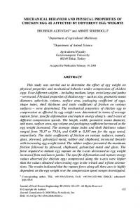
soil deposits of a high northern latitude site on Mars. The soil physical properties component involved the analysis of force data determined from motor currents from the Robotic Arm (RA)’s trenching activity. Using this information and images of the landing site, soil cohesion and angle of internal friction were determined. Dump pile slopes were used to determine the angle of internal friction of the soil: 38° ± 5°. Additionally, an excavation model that treated walls and edges of the scoop as retaining walls was used to calculate mean soil cohesions for several trenches in the Phoenix landing site workspace. These cohesions were found to be consistent with the stability of steep trench slopes. Cohesions varied from 0.2 ± 0.4kPa to 1.2 ± 1.8 kPa, with the exception of a subsurface platy horizon unique to a shallow trough for which cohesion will have to be determined using other methods. Soil on polygon mounds had the greatest cohesion (1.2 ± 1.8 kPa). This was most likely due to the presence of adsorbed water or pore ice above the shallow icy soil surface. Further evidence for enhanced cohesion above the ice table includes lateral increase in excavation force, by over 30 N, as the RA approached ice. Citation: Shaw, A., R. E. Arvidson, R. Bonitz, J. Carsten, H. U. Keller, M. T. Lemmon, M. T. Mellon, M. Robinson, and A. Trebi-Ollennu (2009), Phoenix soil physical properties investigation, J. Geophys. Res., 114, E00E05, doi:10.1029/2009JE003455.

1. Introduction [2] The Phoenix Mars Lander (Scout Mission) landed at 68.22°N, 234.25°E (Areocentric) on May 25th 2008 and operated until 2 November 2008 [Smith et al., 2008]. Phoenix was equipped with a 2.4 m Robotic Arm (RA) that was designed to excavate down to a buried ice table and to acquire and deliver samples of Martian soil to deckmounted instruments [Arvidson et al., 2009]. There are three main types of materials at the site: 1) soil, 2) relatively pure ice, and 3) icy soil. For the first type of material, the term ‘‘soil’’ is used to describe unconsolidated surface material that has undergone various soil formation processes, such as cryoturbation (this practice follows nomenclature developed by Moore et al. [1987]). During the mission, most of the excavation was conducted in this type of material. See Figure 1 for a workspace digital elevation map which includes the trenches and dump piles resulting from RA 1 Department of Earth and Planetary Sciences, Washington University in St. Louis, St. Louis, Missouri, USA. 2 Jet Propulsion Laboratory, California Institute of Technology, Pasadena, California, USA. 3 Max-Planck-Institut fu¨r Sonnensystemforschung, Katlenburg-Lindau, Germany. 4 Department of Atmospheric Science, Texas A&M University, College Station, Texas, USA. 5 Laboratory for Atmospheric and Space Physics, Department of Astrophysical and Planetary Sciences, University of Colorado at Boulder, Boulder, Colorado, USA.

Copyright 2009 by the American Geophysical Union. 0148-0227/09/2009JE003455

activity. Bonitz et al. [2008] gives a review of the RA design and operation. In our paper we use RA trajectory information, retrieval of forces from RA excavations, and images from spacecraft cameras to investigate the physical properties of the soil at the Phoenix landing site. [3] First, background is provided for the landing site, the data sets used, and RA operations. Then we discuss the determination of the first of two Mohr-Coulomb parameters, the angle of internal friction and how it relates to trench slopes. We next review the method of determining the second Mohr-Coulomb parameter: cohesion. This is followed by a description of an example excavation from a laboratory test in a known material, for which the method of Balovnev [1983] yields a reasonable cohesion. We then analyze forces associated with RA excavations in the polygonal landforms at the Phoenix site and retrieve values for soil cohesion. Slope stability calculations are used to demonstrate that retrieved cohesions and angles of internal friction are consistent with trench wall slopes and the absence of wall failures. We then end with a discussion of platy soil that forms a morphologically unique texture relative to the other soil exposures at the landing site.

2. Background [4] The Phoenix lander operated from approximately Ls 77° to 151°. It is the northernmost landed Mars mission to date. The northern plains landing site was chosen because of the prediction of buried water ice based on hydrogen detected in neutron data from the Gamma Ray Spectrometer

E00E05

1 of 19

E00E05

SHAW ET AL.: PHOENIX SOIL PROPERTIES INVESTIGATION

E00E05

Figure 1. Phoenix landing site workspace elevation map after modification by RA. Trenches and dump piles were named after characters and objects in fairy tales and other stories. Trenches discussed in this paper have been outlined in red. The curve in the outline of Stone Soup trench is due to part of the lander blocking the view of the surface. Note the lander footpad toward the lower center. DEM is courtesy of Hanna Sizemore. (GRS) Suite on the Mars Odyssey spacecraft [Boynton et al., 2002] and based on thermal inertia data [Mellon et al., 2008]. Ice table depth (5 cm) observations measured during the Phoenix mission are consistent with current diffusive equilibrium with atmospheric water vapor [Sizemore et al., 2009; Mellon et al., 2008]. Orbital observations also indicate the presence of adsorbed water on surface soil grains [Poulet et al., 2009]. [5] Thermal cracking of the buried icy soil is thought to have led to the formation of meter-scale polygonal trough networks in the overlying soil [Mellon et al., 2009], whose properties are examined in this paper. Throughout this paper, the term ‘‘icy soil’’ is used to indicate the impenetrable (for the scoop blade) ice-cemented soil located underneath a cover of penetrable soil (although, as addressed later, there may be limited pore ice or adsorbed water in this layer as well). Figure 2 shows the RA workspace with approximate polygon outlines drawn in. The RA had access to a shallow polygon trough, a deep trough, the sides of two polygons, and one polygon center, as delineated by Arvidson et al. [2009]. Arrows in Figure 2 indicate where, in relation to these features, ice or icy soil was uncovered. [6] The parent material of the soil was ejecta from Heimdal crater (which is 11.5 km in diameter and located 20 km to the east of the landing site) mixed in with aeolian material [Heet et al., 2009]. The site is in a valley underlain by the Scandia region unit (see Tanaka et al. [2008] for possible formation mechanisms), near the northern boundary of the Alba Patera unit [Heet et al., 2009]. Of

the sites visited by landed missions, the Viking Lander 2 site (at 48° N latitude) is most geologically similar to the Phoenix site, as it is also in the northern lowlands, has a polygonal network, is quite flat [Mutch et al., 1977], and is presumed to have underlying ice. Compared to the other landing sites, the Phoenix site has the lowest rock abundances and least evidence of aeolian processes. [7] Wet chemistry and Thermal and Evolved Gas Analyzer (TEGA) results indicate the Phoenix soil includes carbonate and perchlorate salts and is somewhat alkaline in pH [Smith et al., 2009; Boynton et al., 2009; Hecht et al., 2009; Kounaves et al., 2009]. The soil exhibits the particle size distribution of loamy sand (T. Pike, personal communication, 2009). Particle size distribution can affect apparent cohesion, but the effect is minimal compared to that of interparticle cohesion (loamy sands do not have high apparent cohesion because there is a minimal clay size fraction). Tests where soil clods that were sprinkled onto instrument covers broke apart on contact show that the soil is weakly cohesive, and so there must be an additional contributing factor to cohesion beyond that from particle size [Arvidson et al., 2009]. [8] In this paper, we give numerical estimates of the cohesion and angle of internal friction of the soil. Thus it is useful to look at the magnitude of these parameters at other locations on Mars. The Viking landers encountered soil that was classified into three types: drift, blocky, and crusty to cloddy [Moore and Jakosky, 1989]. Values for cohesion and angle of internal friction for these soil types as well as soils encountered by the Pathfinder and MER rovers

2 of 19


E00E05

E00E05

Figure 2. Phoenix landing site workspace elevation map before modification by RA. Dashed red lines show approximate polygon outlines. Here all trenches excavated during the mission are outlined. Trenches and dump piles were named after characters and objects in fairy tales and other stories. The curve in the outline of Stone Soup trench is due to part of the lander blocking the view of the surface, and the outline of Lower Cupboard is blocked by tailings from Stone Soup. Note the lander footpad toward the lower center of the figure. White arrows point to trenches in which relatively pure ice was found. Purple arrows point to trenches in which icy soil was found. DEM is courtesy of Hanna Sizemore. are given in Table 1. Phoenix soils appear similar to crusty to cloddy soils from the Viking Lander 2 site, as explained in detail by Arvidson et al. [2009].

3. Primary Data Sets [9] There are two primary data sets on which much of the analysis in this paper is based: 1) images of the trenches by cameras onboard the Phoenix spacecraft [Lemmon et al., 2008; Keller et al., 2008] and 2) data acquired by the RA while trenching. The RA is a four degree-of-freedom arm. The degrees of freedom correspond to the four joints, two of which are located in the shoulder and provide motion in azimuth and elevation, and the other two provide motion in elevation for the elbow and wrist. Only the three joints providing motion in elevation were in operation during excavation. Excavation was conducted in a backhoe-style, scooping material toward the lander and lifting it up to be transported to the appropriate dump location. Data from the RA include force values experienced by the RA, time at which those forces were experienced, Cartesian position values for where the RA was located at any point in time, and scoop blade angle values. See Figure 3 for an image of the scoop. Coordinates are in Payload Frame (Zamani et al., Phoenix Software Interface Specification, NASA, Washington, D. C., available at http://an.rsl.wustl.edu/phx/ solbrowser/browserFr.aspx?tab = res, 2008) and refer to the position of the scoop tip. The Payload Frame has its origin

at the RA shoulder (which is at deck level), the x axis points north, the y axis points east, and the z axis points downward (the lander touched down with an orientation such that the side with the RA faced north; this kept icy soil in shadows once exposed). Scoop position was computed based on reported joint angles and the lengths of segments of the arm. The force data were calculated from motor currents, which were measured frequently throughout arm operation. Motor currents were converted to torques via a relation determined by testing and curve fitting. The torque values were then converted to force values via the manipulator Jacobian (the manipulator Jacobian is a matrix obtained by taking the Jacobian of the forward kinematic equations. See Spong

Table 1. Cohesion and Angle of Internal Friction Found for Various Landed Missionsa Mission

c (kPa)

Viking (drift) 0 – 3.7; avg: 1.6 ± 1.2 Viking (blocky) 2.2 – 10.6; avg: 5.1 ± 2.7 Viking (crusty to cloddy) 0 – 3.2; avg: 1.1 ± 0.8 Pathfinder 0.12 – 0.356; avg: 0.238 MER A 5.2 MER B 4.7 – 5.6; avg: 5.13

8(°) avg: 18 ± 2.4 avg: 30.8 ± 2.4 avg: 34.5 ± 4.7 31 – 41; avg: 36.6 30 – 37; avg: 33.5 30 – 37; avg: 33.5

a Note that while the ranges given here are those typical of soils at each site, there were outliers that are not considered in this table. For more information, see Moore and Jakosky [1989], The Rover Team [1997], and Sullivan et al. [2007].

3 of 19

E00E05


E00E05

Figure 3. False color image of Robotic Arm (RA) scoop in Snow White trench. Red arrow indicates direction of lander as well as direction of scoop motion along the bottom of the trench. This convention will be followed to indicate the direction of the lander. Surface Stereo Imager (SSI) image SS051IOF900751600_15C60L21TB. and Vidyasagar [1989] for information on derivation and use). A temperature correction was also applied using a relation based on testing and curve fitting. Resulting force values were broken up into components, of which radial force (Fr) and vertical force (Fz) are used in this paper. Radial force is the lateral force in the direction of excavation. Many of the force values given in this paper are resultant forces (F = sqrt(Fr2 + Fz2)) in the plane that contains the vertical vector as well as the vector pointing in the direction of excavation (Figure 4). Usable force values are sparser than the trajectory values. [10] The data are affected by two sources of oscillation that are systematic effects independent of any soil property. Oscillations in the trajectory data were caused by the algorithm used to determine the intermediate trajectory points in between commanded trajectory points. Oscillations can also appear in the force data; these were caused by the accommodation algorithm. Accommodation occurred when the RA experienced a high level of force; it retreated backward from the ground until the force returned to a value that was considered safe for operation. This accommodation sometimes caused RA trajectory to follow the topography of

the interface between the soil and the underlying icy soil instead of following commanded trajectory. [11] When the RA was in contact with the soil, positions returned in the data were less exact than for moves in free air. When the arm was loaded against the surface, it flexed, resulting in errors in the calculated position. In extreme cases, the error was 2 – 4 cm at the end of the 2.4 m long arm. Relative positioning was generally more accurate than absolute positioning, and positions were repeatable to within 2 mm. [12] Each time a trenching operation was scheduled during the mission, the following parameters were commanded: starting position, trench depth, trench length, trench width, and trench slope, as well as several other parameters. In this paper, each traverse across the bottom of a trench is called a pass. Each trenching command generally resulted in a number of passes (anywhere from one to greater than thirty passes depending on trenching objectives), and each pass attempted to proceed deeper than the previous pass until the commanded depth was achieved. The depth interval between passes was commanded to be different for different trenches. This was done because the trenches are of various lengths and the intent was to ensure

4 of 19

E00E05


E00E05

Figure 4. Schematic of the scoop with superposed vectors showing the direction of forces during excavation. Fx, Fy, and Fz are aligned with the coordinate axes. Fr is the vector sum of Fx and Fy. F is the vector sum of Fr and Fz. Also shown are F1, F2, and F4, the three contributions to horizontal force described in the section on calculating cohesion. F1, F2, and F4 have been lengthened for purposes of illustration, but in reality their magnitudes would add up to that of Fr.

that the scoop did not fill before it reached the end of the trench. Depth intervals between passes ranged from about a third of a centimeter (as was the case for Snow White Trench – most features at the landing site were named after fairy-tale characters) up to one centimeter (DodoGoldilocks Trench). In this paper, each section of a trench that is one scoop width across is called a swath. Many trenches were excavated using multiple trenching commands, and each of these commands often resulted in the creation of multiple swaths (to accomplish this, the RA scoop would generally

pass over one swath, then over the next, and then alternate between the two until the trench was complete). This allowed better viewing of a greater expanse of the trench floor. [13] Another important item to note is that, in general, the angle at which the scoop blade was inclined with respect to the horizontal varied as the RA scoop traveled across the bottom of the trench. For example, sol 76 trenching in Stone Soup had a minimum angle of 116.3°, a maximum of 162.7°, and a mean of 146.1°. Figure 5 illustrates the range

Figure 5. (top left) A 3D schematic of the scoop. (bottom left) A 2D schematic side view. The orange arrows point to the same location on the scoop in each schematic. (right) A diagram of possible blade angle values with the green arrow indicating the orientation of the blade in the 2D schematic (blade level and pointed toward the lander). 5 of 19


E00E05 Table 2. Dump Pile Slopesa Dump Pile

Slope(°)

Transect

Croquet Ground sol 108 north pile Croquet Ground sol 108 middle pile Bee Treeb sol 129 #1 Bee Treeb sol 129 #2 Caterpillar sol 149 Caterpillar sol 117

36.4 29.8 36.8 40.0 47.6 38.8

1 2 3 4 5 6

a See Figure 1 for dump pile locations in the workspace and Figures 6 and 7 for accompanying transects and profiles. These values allow for estimation of the angle of internal friction. b Bee Tree was measured before the platy slabs were dumped on it.

of blade angle values. Although the scoop blade angle varied along each pass (becoming shallower as the pass progressed), in general it did not change from pass to pass.

4. Dump Pile and Trench Wall Slopes and Angle of Internal Friction [14] Table 2 gives slope measurements for various dump piles in the workspace. Figures 6 and 7 show transects and profiles corresponding to each of these slopes. Dump piles have an average slope of 38° ± 5° (same mean is obtained whether or not a von Mises distribution [Jones, 2006] is assumed). The 95% confidence interval assuming a von Mises distribution is used for the estimate of error. The mean dump pile slope is taken to represent the angle of internal friction of the soil because cohesive bonds were broken during the dumping action (clods broke up during

E00E05

sprinkle tests) [Arvidson et al., 2009], however we do not believe that particle shapes were changed. In addition to dump pile slopes, we measured trench wall slopes. Well-lit trench slopes are used to determine an average trench slope value of 71° ± 10° (the 95% confidence interval assuming a von Mises distribution is again used for the error estimate). Furthermore, only sidewalls are used because they were the least affected by compression from the scoop since these walls were parallel to the direction of scoop motion. Table 3 gives slope measurements for various trench walls in the work space, and Figure 8 shows transects and profiles for the walls. Trench wall slopes are much larger than the angle of internal friction, and slope failure was not observed on these walls. This result indicates the presence of cohesive forces in undisturbed soils.

5. Method for Calculating Cohesion [15] In addition to the internal friction, cohesion affects the soil’s resistance to excavation. The analysis in this section follows the methods of Balovnev [1983] to estimate soil cohesion, or shear strength. This technique has been investigated by workers concerned with lunar soils [Wilkinson and DeGennaro, 2007]. Balovnev applied the theory of retaining walls to the walls of a scoop [Balovnev, 1983; Blouin et al., 2001]. He considered draft, or horizontal force, to be made up of four parts: 1) resistance (to cutting) experienced by the blade, 2) additional resistance due to a beveled edge on the blade, 3) resistance (to cutting) experienced by the sides of the scoop, and 4) resistance (from friction) experienced by scoop sides. We neglect part three because scoop passes were not deep enough for this to be a

Figure 6. Profiles used to calculate slopes (given in Table 2) for Croquet Ground and Bee Tree dump piles. The average of the dump pile slopes is then used as an estimate for angle of internal friction. Note that far sides of dump piles were not used since the SSI could not view them. SSI images SS108RAL905790842_0117EL1M1 and SS129RAL907652106_1EC26L1M1. 6 of 19


E00E05

E00E05

Figure 7. Profiles used to calculate slopes (given in Table 2) for Caterpillar dump pile. SSI images SS149RAL909445554_207F6L1M1 and SS117RAL906588190_1D856L1M1. factor. The equations for the remaining parts of the horizontal force are as follows: F1 ¼ wzð1 þ tan d cot bÞA1

F2 ¼ web ð1 þ tan d cot ab ÞA2

zgr þ c cot f ^r 2

eb gr 1 sin f ^r þ c cot f þ zgr 2 1 þ sin f

zgr F4 ¼ 4 tan dA4 ls z þ c cot f ^r 2

where A1 = A(b), A2 = A(ab), and A4 = A(p/2). pffiffiffiffiffiffiffiffiffiffiffiffiffiffiffiffiffiffiffiffiffiffiffiffiffiffiffiffi cos d cos d þ sin2 f sin2 d AðbÞ ¼

1 sin f

1 sin d exp 2b p þ d þ sin tan f sin f

ð1Þ

where w is blade width, z is depth between passes (i.e., excavation depth), d is the soil scoop friction angle, b is the rake angle, 8 is the soil friction angle, g is Mars gravity, r is bulk density, c is cohesion, eb is the height of the blunt (beveled) edge, ab is the angle of the blunt edge, ls is the length of a scoop side, and ^r indicates that the listed contributions to the force are all in the horizontal, radial direction. [16] Here we compare horizontal force values resulting from the above equations to the horizontal force returned in the RA telemetry in order to obtain soil cohesion values. The first excavation in Snow White is used to illustrate the procedure for determining cohesion.

[17] Some assumptions are made in order to attain cohesion values. 1) The scoop blade angle varied along the length of each trench as it was being excavated. For example, for the first excavation into Snow White, the angle varied from 123.2° to 169°, with an average of 147.3° (to obtain rake angle, this value as well as values given for other trenches must be subtracted from 180°). This average value is used in calculations, and the angle of the beveled end of the scoop blade is also taken into account (see Figure 5). The scoop blade is at an angle relative to the rest of the scoop, but its angle is used in calculations of cohesion because the thickness of each tract of soil being excavated in a single pass is generally less than the scoop blade length (some sample acquires are exceptions). 2) The angle of external friction (soil scoop friction) is assumed to equal the angle of internal friction as it is assumed that after the first excavation the scoop was no longer clean. 3) Density is assumed to be 1.235 g/cc from Thermal and Electrical Conductivity Probe observations [Zent et al., 2009] (uncertainty in this value is due to instrument error as well as to the following assumptions: basaltic mineralogy, no soil disturbance from needle placement). This density

Table 3. Trench Wall Slopesa Trench Wall

Slope(°)

Shadowed

Transect

Snow White sol 108 north wall Snow White sol 108 south wall La Mancha sol 148 left wall La Mancha sol 148 right wall Upper Cupboard sol 147 left wall Upper Cupboard sol 147 right wall DodoGoldilocks sol 149 right wall DodoGoldilocks sol 116 left wall

65.6 61.7 66.7 71.6 58.3 79.4 57.1 83.4

no yes yes no yes no no no

7 7 8 9 10 10 N/A N/A

a See Figure 1 for trench locations in the workspace; Figure 8 shows accompanying transects and profiles for a sampling of the trenches.

7 of 19

E00E05


E00E05

Figure 8. Profiles used to calculate slopes (given in Table 3) for trench walls. SSI images SS108RAL905790842_0117EL1M1, SS148RAL909363043_20566L1M1, and SS147RAL909270572_ 20456L1M1.

value is consistent with the density Moore and Jakosky [1989] found for similar crusty to cloddy soil at the Viking landing sites [Arvidson et al., 2009]. Deviations from this value are taken into account in the calculation of the uncertainties. 4) The depth between passes is taken from the parameter set used in commanding the RA. Other values used include: gravity (3.76 m/s2), blade width (8.6 cm), beveled edge thickness (0.093 cm for a horizontal blade), beveled edge angle to rest of blade (34.8°), and side length (11.4 cm). Balovnev’s [1983] equations give horizontal force required to excavate through soil of a given cohesion. We solve his equations for cohesion so that we can work backward and use the horizontal force values (Fr – force in the direction of excavation) returned by the RA to obtain the soil cohesion. Only negative forces are used in the Fr distributions because the negative direction in the RA coordinate system is toward the RA shoulder (i.e., toward the lander) and the backhoe motion of the RA is toward the lander as well. Positive values are most likely rebound values due to the fact that the RA is a mechanical system; so positive values are ignored since they do not reflect soil

properties. If excavation activity involved significant accommodation, data points from the section of the trench where this happened are removed before horizontal force is averaged. Table 4 gives cohesions for various trenches in the workspace, uncertainties in cohesion, values of the various contributions to force described earlier, and values of certain other parameters used to calculate cohesion. Uncertainty in horizontal force, density, rake angle, angle of internal friction, depth between passes, and gravity estimate are taken into account in the error propagation calculations. The uncertainty in horizontal force results in the largest contribution to the uncertainty in cohesion; uncertainty in angle of internal friction gives the second largest contribution. Note that the uncertainties in cohesion are larger than the calculated values. While this means that there is no reliable lower bound (other than 0 kPa) for those values, it still gives the most likely value as well as an upper bound. Furthermore, the relative error in cohesion values is less than the absolute error given here. In general, higher uncertainty values are obtained when using excavation models to determine cohesion, as opposed to using a direct

8 of 19

E00E05


E00E05

Table 4. Average Cohesions From Various Trenchesa Excavation

SW22d1 Soil

SW22d2 Soil

ISd1 Soil Portion

UC67 Soil

UC67 Ice-Affected Soil

Fr (horizontal force; N) z (depth between passes; m) th (blade angle; °) F1 (N) F2 (N) F4 (N) 2sigma uncertainty in Fr (N) Resulting cohesion (kPa) Error estimate for c (kPa)

8.96 0.0030 147.25 0.86 0.41 7.69 10.66 0.6 0.8

12.07 0.0020 149.44 1.13 0.79 10.15 16.17 1.2 1.8

12.11 0.0060 151.00 1.18 0.27 10.67 16.59 0.4 0.7

3.22 0.0029 161.57 0.32 0.12 2.78 4.69 0.2 0.4

9.58 0.0029 141.95 0.95 0.48 8.14 17.15 0.6 1.2

Excavation

LM132d2 East

SS74

SS76

SS85

SS88

Fr (horizontal force; N) z (depth between passes; m) th (blade angle; °) F1 (N) F2 (N) F4 (N) 2sigma uncertainty in Fr (N) Resulting cohesion (kPa) Error estimate for c (kPa)

4.78 0.0050 162.18 0.48 0.11 4.19 10.28 0.2 0.5

3.89 0.0029 146.10 0.38 0.19 3.33 6.79 0.3 0.5

3.39 0.0029 146.10 0.33 0.16 2.90 6.45 0.2 0.5

4.60 0.0029 143.81 0.45 0.23 3.92 5.69 0.3 0.5

5.12 0.0029 139.80 0.52 0.27 4.34 9.05 0.3 0.7

a Italicized rows indicate average cohesions from various trenches. Parameters used to calculate cohesion are also listed. The above use 1235 kg/m3 density, 8.6 cm blade width, 3.76 m/s2 gravity. Note that the error given corresponds to the average cohesion and there are gradients within the populations. SW, Snow White; IS, Icy Soil; PIT, Payload Interoperability Test bed Test; UC, Upper Cupboard; LM, La Mancha; SS, Stone Soup. Numbers after each of these abbreviations stand for the sol of the activity. d1 = dig1. d2 = dig2. See the text for descriptions of parts F1, F2, and F4 of the force. Part 3 is not used because the passes were not deep enough for sidewall cutting action to be a factor.

shear test, which is relatively impractical for a planetary mission; for an example of uncertainties resulting from modeling a similar process, see Moore and Jakosky [1989].

6. Payload Interoperability Test Bed Experiments [18] Before discussing the cohesion of the landing site soil, we present results from laboratory testing in a loose soil over a hard icy soil simulant. Figure 9 shows the RA trajectory for the first excavation in the University of Arizona Payload Interoperability Test bed (PIT) icy soil simulant trenching test conducted with an engineering model of the spacecraft. During each pass of the trenching activity, the scoop moved from the far edge of the trench toward the depth axis or z axis (which intersects with the RA shoulder at depth = 0 m). This means that, in Figure 9, as well as in all of the trajectories that will be shown in this paper, the RA scoop comes down on the right side, travels through the soil, and then turns upward and is elevated out of the trench when it gets to the left side. Most of this first excavation was through the soil simulant used to cover the hard icy soil simulant. The Mars soil simulant used was poorly sorted basaltic soil (silt-sized up to 150 mm diameter particles with sand being the predominant fraction) that retained its shape after compression; this was due to the fine grain fraction which fills in the pore space giving the soil an apparent cohesion. The method of Balovnev yields a cohesion of 0.4 ± 0.7 kPa (Table 4) for this soil. This soil is shown in Figure 10 as the darker soil in the upper layer, above the lighter-toned material representing the hard icy soil simulant. The lineations, or chatter marks, are due to interaction of the soil with the RA during excavation. Note that lineations such as this have also been seen on the floors of trenches at the landing site [Arvidson et al., 2009]. When the RA reached the lighter-

toned icy soil simulant, it could not penetrate into the simulant with the scoop blade and instead underwent stick slip motion where it skittered across the surface. Figure 10 shows that higher forces resulted when this happens. This same stick slip motion occurred when the RA scoop blade passed over the surface of icy soil at the landing site, so an icy soil rasp was used to penetrate and acquire icy soil [Arvidson et al., 2009].

7. Excavation at the Side of a Polygon [19] Both the first touch, which consisted of pressing the bottom of the RA scoop into the soil, and the first excavation into the soil at the landing site were conducted on the side of a polygon at the site of what is now a trench named DodoGoldilocks (Figures 1 –2). For analysis of soil on the side of a polygon, we used a trench named Upper Cupboard (which was excavated immediately to the east of the DodoGoldilocks trench) because its excavation was conducted at more frequent depth intervals and more data points were obtained than for DodoGoldilocks; therefore, it gives a better indication as to the strength of the soil. Figure 11 shows the trajectory with force values for the first excavation of Upper Cupboard trench, conducted on sol 67. Forces grade from high to low as the location of the scoop progresses away from the deeper section of the far end of the trench. The RA went into safe mode in that area of the trench, and was covering most of the exposed ice when the trench was imaged. However, in an image from a later sol, the location of the ice was found to correspond to the location of many of the highest force values (Figure 12). Therefore, the relatively pure ice found in Upper Cupboard (and in DodoGoldilocks) has a significant effect on the strength of the soil located in the same section of the trench. This soil has a cohesion of 0.6 ± 1.2kPa (Table 4). Any

9 of 19

E00E05


Figure 9. Excavation one of the Icy Soil PIT Test. The cement icy soil simulant is not actually encountered until excavation two (see Figure 10). Red arrow gives direction of lander. Vertical lines represent free space moves where the scoop is entering or leaving the trench. The color-coded stars represent locations along the trajectory for which force data (in the direction of the lander) was returned. Note that force does not increase with depth or with proximity to underlying hard cement layer.

Figure 10. Laboratory testing which involved using the Robotic Arm to dig through Mars soil simulant and then buried cement icy soil simulant. The red line represents an approximate division between the two. Also shown is a close overlay of force values from part 2 of the excavation (part 1 is shown in Figure 9). As can be seen from the color-coded data points, forces are much higher over the icy soil simulant; this indicates the relative hardness of the material. Red arrow gives direction of lander. Note that additional tests were performed on this trench between when the force data was collected and when the image was taken, this includes activities that formed the deeper striations in the middle of the trench. 10 of 19

E00E05

E00E05


E00E05

granular material has a similar cohesion to the values listed in Table 4 [Scholtes et al., 2009].

8. Excavation at the Center of a Polygon

Figure 11. Trajectory color coded by force for trenching in Upper Cupboard on sol 67. Red arrow gives direction of lander. Note the increase in force toward the lower far side of the trench (to the right) and compare with the location of ice in Figure 12. chunks of ice that may have been excavated would have affected this value. Soil on the opposite side of the trench has a cohesion of 0.2 ± 0.4 kPa. See Table 4 for parameters used in the calculation. For rough comparison, loose,

[20] On the first sol that we trenched in the center of a polygon (Wonderland polygon mound), icy soil was revealed and verified spectroscopically [Blaney et al., 2009]. The icy soil (seen in Snow White trench, Figure 13) is believed to correlate with accommodation seen in the RA trajectory, and this is used to differentiate between icy and relatively non icy soils in the RA force data. Two excavations were conducted in Snow White on Sol 22 (the first sol of RA activity in this region). For the cohesion calculations, force values taken from the first excavation (maximum depth below surface: 3 cm) are used to represent shallow soil; calculations using these values result in a cohesion of 0.6 ± 0.8kPa. The deep soil force data are taken from the second excavation (3 –5 cm depth below surface) and result in a cohesion of 1.2 ± 1.8kPa. However, even before the RA began its second excavation, there was a change in soil cohesion; this can be seen through a decrease in scoop velocity as the excavation progressed (See Table 5). Velocity is calculated from position and time data returned by the RA. Of the net 2 cm/s velocity decrease over the ten passes analyzed, 1.7 cm/s velocity change occurred over the course of only three passes (passes 5 – 7). This corresponds to the depth at which we start seeing higher forces [Arvidson et al., 2009, Figure 19] that are not associated with accommodation. This change is abrupt and velocity does not change appreciably from pass to pass in the second

Figure 12. Upper Cupboard trench. Ice is evident in the upper right section of the trench. Red arrow gives direction of lander. SSI image SS084IOF903660997_19CA0L21TB. 11 of 19

E00E05


E00E05

Figure 13. Snow White trench. (left) Contrast has been sacrificed in preference for approximate true color. (right) A false color image (SSI filters 10, 11, and 12) (available at http://an.rsl.wustl.edu/phx/ solbrowser/browserFr.aspx?tab = res) gives a clearer view of darker areas of the trench floor that mark the presence of icy soil. A morphological expression of surface cohesion can be seen in the red circle. Red arrow gives direction of lander. SSI image SS022IOF898161657_12CAERCBA1TB.

excavation into Snow White (on the same sol). The previous example of Upper Cupboard trench indicates that we would expect a more gradual gradient if this were due to proximity to the ice table. As will be discussed in a subsequent section of this paper, we do also see a gradual gradient that appears to be related to proximity to ice at Snow White; this change appears in the form of an angled gradient in force. [21] Both the first and second trenching activities conducted on Sol 22 in Snow White exhibit accommodation and therefore both encountered icy soil corresponding to the ice table. We can see this from the higher forces experienced by the RA in an area toward the foot of the trench where the trajectory measurements also show the arm moving higher in elevation, i.e., experiencing accommodation (Figure 14). Force values show that the ice table is uneven, despite trenching on relatively flat land at the top of a polygon. The posttrenching image also shows this pattern (Figure 13). For regions where the RA encountered icy soil that it cannot penetrate, spectra indicate 30% ice and 70% soil [Cull et al., 2008]. We do not present cohesion values for this icy soil (beneath the ice table) because the RA was not able to excavate into that material with the scoop blade. If data points for which the arm accommodated to this icy soil are excluded, we can still see that the overlying soil at Snow White has relatively high cohesion, i.e., the material in Snow White is generally more difficult to trench than material at the sides (Upper Cupboard trench) and troughs (Stone Soup and La Mancha trenches) of polygons. This may be partially due to a higher level of soil processing on polygon mounds, but appears to be closely related to the proximity of the ice table. This effect can be seen in Figure 14, where there are higher

forces in the foot of the trench (the area where the icy soil causes arm accommodation at the floor). These forces are evident right up to the surface in this section of the trench. This effect may be due to the RA encountering more pore ice or more adsorbed water as it progresses closer to the impenetrable icy soil.

9. Excavation in a Deep Trough [22] On the opposite side of the terrain elevation spectrum from Snow White trench, the Stone Soup trench is located in a polygon trough. During the first four sols of trenching activity in Stone Soup, the RA scoop alternated, first trenching along the right, then trenching along the left of

Table 5. Velocity Change With Deptha Depth Level

Scoop Velocity (cm/s)

D v (cm/s)

1 2 3 4 5 6 7 8 9 10

3.48 3.43 3.35 3.35 2.91 2.27 1.65 1.61 1.53 1.42

0.05 0.08 0.00 0.44 0.64 0.63 0.04 0.08 0.10

a Depth levels corresponding to a lower pass than the previous one by 0.3 cm. This information is for the first of two sol 22 excavations conducted in Snow White. The rows in bold represent large amounts of velocity change. This occurs roughly 1.5 – 2 cm below the surface.

12 of 19

E00E05


E00E05

Figure 14. Trajectory followed by the RA in the first excavation in Snow White trench. The stars represent locations along the trajectory for which force data (in the direction of the lander) was returned. Red arrow gives direction of lander. Note the higher forces on the landerward side of the trench, near the icy soil. the trench. Each sol’s activity consisted of 12 passes along each side of the bottom of the trench. In order of depth below the surface (also sol order), calculated cohesions for Stone Soup are: 0.3 ± 0.5kPa, 0.2 ± 0.5kPa, 0.3 ± 0.5kPa,

0.3 ± 0.7kPa (Table 4). Taken together, the cohesions, and especially the force distributions (Figure 15), from the latter two sols show that force increased with depth. However, there is no spectral confirmation that the scoop ever reached

Figure 15. Trajectory color coded by force for Stone Soup trench from sols 74, 76, 85, and 88. Force is the total force in the plane of excavation. Vertical lines represent free space moves where the scoop is entering or leaving the trench. Red arrow gives direction of lander. Note the higher forces near the bottom of the headwall. 13 of 19


E00E05

E00E05

Figure 16. (left) The DodoGoldilocks trench before its western wall was stressed by pushing the bottom of the scoop into the soil. (Right) An image taken after. (middle) A close-up of the affected section of the wall. The imprint of the scraper blade and of the load plate around the rasp can also be seen. Also note the cracks in the upper left of the close-up image. SSI images SS116IOF906529195_1D720RCBA1TB and SS116IOF906500372_1D650RCBA1TB. RAC image RS116RAL906506990_1D77EMBM1. the ice table since the floor of the trench was in shadow (also note that the RA did not experience accommodation). Figure 15 shows the variations in the force profile of the trench (from first four sols of excavation). The scoop may have hit part of the ice table or a hard soil clod at the bottom of the trench’s head wall, where Figure 15 shows exceptionally high forces, exceeding 100 N.

10. Slope Stability [23] A slope stability experiment was conducted near Stone Soup, at the southern portion of the western wall of DodoGoldilocks. This was the only location where a wall was stressed with the intent to initiate slope failure (Figure 16). Despite the application of 75 N vertical force with the bottom of the RA scoop, slope failure was not observed on the wall. We can therefore use this experiment to estimate the minimum amount of cohesion the soil must have in order to withstand the applied stress. This is the cohesion at which the stressed wall would have a Factor of Safety (FoS) of unity. GALENA [Clover Technology, 2006] slope stability modeling software was used to model stresses and slope failures using limit equilibrium analysis on a 2D slope with a Mohr-Coulomb soil description. Properties and bounds defined in the model include: cohesion (varied), angle of internal friction (38°), unit weight (1235 kg/m3 3.76 m/s2 = 5.264 kN/m3), slope failure type (circular or noncircular), failure surface bounds and radius, stress value, extent of stressed area, and analysis type (Spencer or Bishop analysis) [Spencer, 1968; Bishop, 1955]. Varying analysis type did not change the results significantly. Neither did taking into account the presence of a harder subsurface layer. Multiple forward analyses were conducted on the model until the surface with a FoS just above 1 (the critical failure

surface) was found, however this surface is a trivial case (Figure 17, bottom); if failure occurred at this surface, it would not be identifiable in digital elevation map data. A spectrum of failure surfaces from one that would not be noticed to one that involves the whole area of material under the scoop were investigated (Figure 17) and yield a range for minimum cohesion from