Phylospaces: Reconstructing Evolutionary Trees in Tuple Space

Phylospaces: Reconstructing Evolutionary Trees in Tuple Space Marc L. Smith1 and Tiffani L. Williams2 1 Colby

College Department of Computer Science Waterville, ME 04901-8858 USA [email protected]

Abstract Phylospaces is a novel framework for reconstructing evolutionary trees in tuple space, a distributed shared memory that permits processes to communicate and coordinate with each other. Our choice of tuple space as a concurrency model is somewhat unusual, given the prominence and success of pure message passing models, such as MPI. We use Phylospaces to devise Cooperative Rec-I-DCM3, a population-based strategy for navigating tree space. Cooperative Rec-I-DCM3 is based on Rec-I-DCM3, the fastest sequential algorithm under maximum parsimony. We compare the performance of the algorithms on two datasets consisting of 2,000 and 7,769 taxa, respectively. Our results demonstrate that Cooperative Rec-I-DCM3 outperforms its sequential counterpart by at least an order of magnitude.

1

Introduction

Phylospaces is a novel framework that significantly improves the performance of existing phylogenetic methods by employing the power of cooperation. A phylogeny is an evolutionary tree that attempts to relate the common ancestry of a set of organisms, or taxa. In such a tree, the taxa occupy the leaf nodes, and the branches and interior nodes represent the relationships between the taxa. It is impossible to know the true evolutionary history for a given set of taxa. Moreover, for n taxa, there are (2n − 5)!! hypotheses (i.e., unrooted binary trees) that could explain the evolutionary history of these organisms. The most popular approaches for inferring phylogenies use NP-hard optimization criteria such as maximum likelihood (ML) and maximum parsimony (MP). Phylogenetic heuristics try to find the best trees, based on an optimization criterion, and and a strategy for exploring the search space. Most implementations of phylogenetic heuristics

1-4244-0054-6/06/$20.00 ©2006 IEEE

2 Texas

A&M University Department of Computer Science College Station, TX 77843-3112 USA [email protected]

are sequential; most parallel phylogenetic methods focus on ML techniques. Within Phylospaces, we designed Cooperative Rec-I-DCM3 [17], a parallelized version of RecI-DCM3 [13], the best-performing MP heuristic for phylogeny reconstruction. Maximum parsimony is an optimization criterion based on Occam’s Razor, so named for William of Occam. Applied to scientific theories, Occam’s Razor is also called the principle of parsimony. This principle advises us to choose the simplest explanation for a phenomenon. Applied to phylogenies, for a given set of taxa, the evolutionary tree(s) with the least number of changes (mutations) among the taxa are considered to be the most accurate. We compared the performance of Rec-I-DCM3 and Cooperative Rec-I-DCM3 on two datasets consisting of 2,000 and 7,769 taxa. In our experiments, Cooperative Rec-IDCM3 demonstrated a consistent and dramatic improvement in performance over its sequential counterpart, RecI-DCM3. We chose Rec-I-DCM3 as a basis for comparison because we were curious if it would be possible to improve upon the best established MP heuristic. Our experiments with Cooperative Rec-I-DCM3 showed improvement by at least an order of magnitude to best-known MP scores. The reason for Cooperative Rec-I-DCM3’s success is the cooperation supported by the Phylospaces framework. Cooperative Rec-I-DCM3 is a population-based strategy that emerged from the authors’ respective visions regarding cooperation, and after considering different approaches to parallelism. One goal was to leverage the power of cluster computing with existing phylogenetic heuristics by maintaining a diverse population of trees (i.e., a tree pool) that could be refined over successive iterations by multiple instances of some existing sequential heuristic. The nature of the task and the tree pool caused us to consider several possible parallel and distributed computing approaches. In the remainder of this section, we describe what led us to choose Tuple Space, a distributed shared memory model.

Tuple space is part of a very different model of concurrency, named Linda [6] . The Linda model is not precisely shared memory, nor is it exactly a message passing model. Linda is a hybrid model of concurrency, dubbed by its creator, David Gelernter, as generative communication. The role tuple space plays in the Linda model is that of a distributed, shared memory. It turns out that tuple space is a very natural and convenient environment for implementing Phylospaces. The thought of implementing a tree pool among processes through message passing was distracting, while the possibility of running our experiments on a shared memory multiprocessor was cost prohibitive. The distributed shared memory model supported by Linda and tuple space was the ideal compromise, and permitted us to build and run our experiments on low-cost commodity clusters. We take a cooperative approach to developing parallel algorithms for phylogenetics. Although most of the attention has been given to ML [3, 5, 9, 10, 15], there are a few parallel algorithms for MP [2, 4]. Without the help of parallelization, ML approaches are extremely slow, limiting their use to small problems. The ML estimate of a phylogeny is the tree for which the observed data are most probable. Many biologists prefer ML since it is statistically well-founded, possibly producing the most accurate phylogenetic trees. However, many biologists prefer MP approaches and believe in the accuracy of the resulting trees.

2

Linda and Tuple Space

The Linda model [6] is a model of concurrency based on a distributed shared memory, known as tuple space, and the process coordination language Linda. Models of concurrency—including parallel and distributed—typically fall into one of two main categories: shared memory and message passing. Linda’s unusual properties, however, don’t permit such ready classification. According to Gelernter, the Linda model is an example of a new category of concurrency that he dubbed generative communication.

2.1

Generative Communication

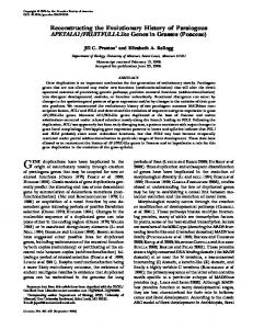
Generative communication exhibits what Gelernter called communication orthogonality—communications that are decoupled in three dimensions: destination, space, and time. Destination decoupling refers to communications with anonymous senders and receivers. Senders don’t know who will receive their messages, and receivers don’t know who produced the information they receive. Space decoupling refers to communication heterogeneity, or architecture independence among communicating processes. Because tuple space is an associative memory, tuples have no notion of an address in memory—they are matched based on the

P1

P4

rd( "maxprimes", ?val )

out( "array", "primes", "nextindex", 5 )

( "array", "primes", "nextindex", 5 ) ( "maxprimes", 100 )

( "array", "primes", 3, prime(3) )

("array", "primes", 0, 2) ( "array", "primes", 4, prime(4) ) ("array", "primes", 1, 3) ("array", "primes", 2, 5)

in( "array", "primes", ?int, ?int)

P2

eval( "array", "primes", 4, prime(4) )

P3

Figure 1. Linda processes interacting in Tuple Space.

sequence and types of the data they contain. Thus, there are no pointers, which tend not to be portable across computer architectures. Time decoupling refers to the ability of processes to communicate with one another, even if they do not execute at the same time. A process generates data (hence, generative communication) and places it in tuple space with one of the Linda primitives. The process that eventually consumes this data need not yet exist at the time the data is produced. A process that wishes to consume data does so by matching a tuple in tuple space with one of the Linda primitives. The process that produced the tuple it matches may long since have ceased to exist! Collectively, communication orthogonality means that processes unknown to each other, running at different times on different computer architectures, may communicate with one another. Designing a concurrent system using the Linda model leads to loosely coupled systems, which tend to be maintainable and extensible over time. For example, Lindabased programs are largely shielded from changes in hardware, operating systems, network topology, and even programming languages.

2.2

Linda Primitives

Linda is an elegant process coordination language consisting of four primitive operations on tuple space: rd(), in(), out(), and eval(). As a coordination language, Linda is intended to augment existing sequential computational languages, such as C, Fortran, and Java. For example, CLinda is the C language augmented with the Linda primitives. Using C-Linda, a programmer can compose pro-

grams consisting of multiple concurrent processes. These processes communicate and coordinate with one another through the medium of tuple space, using nothing more than the four Linda primitives. We refer to Figure 1 in the following description of Linda primitives and tuple space. Figure 1 depicts tuple space as a cloud. Four processes (P1, P2, P3, and P4) surround the cloud, which in turn envelopes a number of tuples. As the naming suggests, tuples are the natural elements of tuple space. A tuple is an ordered sequence of typed values, or value-yielding computations. Tuples in Figure 1 are represented by parenthesized lists of values, delimited by commas. It is sometimes convenient to refer to the values of a tuple by the field in which it resides. For example, (”maxprimes”, 100) is a tuple consisting of two fields, the first of which contains a string of characters (a variable name), the second contains an integer (the variable’s corresponding value). A valueyielding computation is represented by a function call, indicating a value still being computed. For example, the tuple (”array”, ”primes”, 3, prime(3)) is a tuple consisting of four fields; the first two fields contain strings (indicating an array type, and name of array), the third field contains an integer value (array index), and the fourth will contain the result of computing prime(3) (the value to be stored in index location 3). The tuples in Figure 1 represent an example of a distributed data structure, an array. Tuples that contain one or more value-yielding computations are considered active; tuples whose values have all been computed are considered passive. Only passive tuples are visible in tuple space—eligible for matching by other Linda processes. Active tuples become passive once the last value-yielding computation in one of its fields has been computed. The primitives eval() and out() are asynchronous (non-blocking) and permit processes to place active and passive tuples, respectively, in tuple space. Thus, eval() is used to create new Linda processes, since Linda processes are value-yielding computations. The primitives rd() and in() are synchronous (blocking) and attempt to match, then copy or remove passive tuples, respectively, from tuple space. If no match is found in tuple space, the Linda process issuing rd() or in() blocks until a match exists. Sources of nondeterminism should be mentioned. Nondeterminism is a natural consequence of parallel and distributed computation. The careful reader may notice that P2’s in() operation might match one of a number of possible tuples in tuple space. In fact, the tuple that is matched is nondeterministic. In this example, the operation could have matched any of the three tuples with ”array” as the first field, ”primes” as the second field, and an integer in the third and fourth fields (e.g., (”array”, ”primes”, 1, 3)). One additional source of nondeterminism not depicted in Figure 1 involves two or more Linda processes attempting to match the same

tuple at the same time. In this case, it would be nondeterministic which one succeeds.

3 Evolutionary Trees and Tuple Space Phylospaces is a new infrastructure for reconstructing phylogenetic trees quickly and accurately. It’s novelty lies in using tuple space as a vehicle for phylogenetic methods to share their results with each other. The remainder of this section describes Phylospaces along with a description of Cooperative Rec-I-DCM3 [17], our first cooperative algorithm implemented within the Phylospaces framework.

3.1

Phylospaces

An algorithm within Phylospaces consists of the following steps. 1. Create a population of µ initial tree solutions. 2. For each of the µ trees, run a phylogenetic heuristic of choice. 3. Create a new tree population by performing selection and recombination on the trees from step 2. 4. Repeat steps 2 and 3 for the desired number of iterations. Figure 2 provides an illustration of an iteration in Phylospaces. Here, the size of the population (or µ) is four. Each solution is represented by a tuple with three fields: a tag name, tree identifier, and tree score. Hence, the starting tree pool consists of the trees t 1 ,t2 ,t3 , and t4 and their corresponding scores of 39, 35, 40, and 42. The iteration begins by applying a phylogenetic local search heuristic to each solution in the starting tree pool. Since Phylospaces is written for a parallel and distributed environment, the µ local searches can be performed concurrently. Hence, each local search is executed by an lsearch worker, who retrieves a tree from the starting tree pool using the in() operation. Afterwards, the resulting tree from the local search is placed into tuple space with an out() operation. The local search heuristic may not improve the score of the tree it receives. In Figure 2 the scores for t 1 ,t2 , and t2 , are not improved during the local search phase. In the case of t 4 , the score is actually worse. The merger phase begins by collecting all of the results obtained from the local search phase. Here, a merger worker employs a selection and recombination scheme to the population of trees in the local search tree pool. In Figure 2, t1 and t2 have been selected to appear in the final tree pool without any further modifications, whereas trees t 3 and t4 will be replaced by new trees formed by recombining subtrees into a single tree. In our example, t 3 will be replaced by the recombination of trees t 2 and t4 (i.e., t2 ◦t4 ), and t2 ◦t4

("tree", t1, 39) ("tree", t2, 35) ("tree", t3, 40)

("lsearch", t3, 39)

1

lsearch[i]: in("tree", ...) local search out("tree", ...)

("tree", t4, 42)

Tuple Space (starting tree pool)

1

("tree", t2!t4, 50)

4

("lsearch", t4, 47) ("lsearch", t1, 39) ("lsearch", t2, 35)

merger: selection and recombination

4

("tree", t1!t3, 48) ("tree", t1, 39) ("tree", t2, 35)

Tuple Space (local search tree pool)

Tuple Space (merged tree pool)

Figure 2. One iteration of the cooperative algorithm used by Phylospaces. The number of solutions (or µ) in tuple space is four. We also assume that the number of lsearch workers is four. Hence, each phylogenetic heuristic is responsible for processing one tree. The merger worker performs selection and recombination on the population of trees from the local search phase, which results in the merged tree pool. The recombination of two trees is represented by the composition operator (◦). Thus, in the final population one tree is the result of the recombination of t 1 and t4 . The other tree results from the recombination of t1 and t3 .

replaces t4 . Once the merging phase is finished, an iteration in Phylospaces is complete. Although Figure 2 shows that each lsearch worker is responsible for only one tree, it can handle situations where the number of trees (µ) is greater than the number of lsearch processes (p). In such cases, each lsearch worker will receive µp trees from the tree pool. However, there is only one merger worker in Phylospaces who is responsible for selection and recombination. Future modifications will accommodate the parallelization of the merging phase. Implementation: Besides one merger and p lsearch workers, there is also one startup and p seed workers. Each seed worker is responsible for creating µp initial trees using any method of choice. For those familiar with the master-worker paradigm, startup acts as the master process. It is responsible for overseeing computation within Phylospaces. Hence, startup initiates the execution of the other workers (i.e., seed, lsearch, merger) by using the eval() operation.

3.2

Cooperative Rec-I-DCM3

Phylospaces presents a general model for expressing cooperative phylogenetic heuristics. We explore the performance of Rec-I-DCM3 [12]—the best-performing MP heuristic to-date—within our cooperative framework. We call our new algorithm Cooperative Rec-I-DCM3 [17]. Experimental results show that Rec-I-DCM3 outperforms PAUP [16] and TNT [7] by at least an order of magnitude.

Rec-I-DCM3 comes from a family of Disk-Covering Methods (DCMs) [8, 11, 13] that have been successfully applied to reconstructing phylogenetic trees quickly and accurately. Collectively, DCMs are an example of divide-andconquer algorithms that consist of four main stages: (i) decomposing the original dataset into subproblems, (ii) solving each of the subproblems with a base method of choice, (iii) merging the subproblems into a single solution on the original dataset, and (iv) refining the merged tree into a binary tree. Rec-I-DCM3 combines both recursion and iteration to provide a powerful technique for searching tree space. The recursive application of the decomposition step produces smaller and smaller subproblems until every subproblem is small enough to be solved directly. Once the dataset is decomposed into overlapping subsets, subtrees are constructed for each subset and combined using the Strict Consensus Merger [8] to produce a tree on the combined dataset. In Cooperative Rec-I-DCM3, each lsearch worker uses the Rec-I-DCM3 algorithm as its local search algorithm. The selection and recombination algorithm employed by the merger worker is as follows. For selection, the µ trees from step 2 are ranked based on their MP scores, with the best scoring MP tree having the best rank. Next, the trees are placed into sets (A, B, and C) based on their rank. The algorithm also keeps a list of elite solutions (i.e, the best trees found so far). These elite trees are placed into set A; top-ranking trees from step 2 are placed into set B. The remaining lower-ranking trees are put into set C. These trees comprise the new population that is subjected to recombination.

Trees in set C may be recombined with trees in A ∪ B to create new (and more diverse) solutions. If t ∈ C is chosen for recombination, it will be replaced by the resulting tree from the recombination phase. For each tree t ∈ C, there is a p% chance that it will undergo recombination with a random tree t % ∈ A ∪ B. (In our experiments, p = 20%.) t and t % are recombined by computing their strict consensus tree, which contains all of the bipartitions that are common between the trees. Since the strict consensus tree typically results in a multifurcating tree, it is refined into a binary tree and subjected to a global search using Tree-Bisection and Reconnection (TBR).

3.3

Non-cooperative algorithms

Phylospaces can also accommodate a population of heuristics that operate independently. For example, in an experimental setting, it is typically necessary to execute multiple runs of a heuristic. Since each run of the heuristic operates independently, there is no need for a merger worker. We used this approach for our experiments with Rec-I-DCM3 as we were able to execute five independent runs of the algorithm concurrently in the Phylospaces environment.

4

Experimental Methodology

Datasets: Our experiments compared the performance of the algorithms on two biological datasets. Below, we provide the details of both datasets, along with their bestknown score under maximum parsimony, since the optimal score is not known. 1. A set of 2,000 aligned Eukaryotic sRNA sequences (1251 sites) obtained from the Gutell Lab at the Institute for Cellular and Molecular Biology, The University of Texas at Austin. Our runs of both Rec-I-DCM3 and Cooperative Rec-I-DCM3 established a best score of 74,534. 2. A set of 7,769 aligned ribosomal RNA sequences (851 sites) from three phylogenetic domains, plus organelles (mitochondria and chloroplast), obtained from the Gutell Lab at the Institute for Cellular and Molecular Biology, The University of Texas at Austin. The best score for this dataset is 99,794, which was established by Cooperative Rec-I-DCM3. Experiments: All experiments consisted of five runs of the Rec-I-DCM3 and Cooperative Rec-I-DCM3 algorithms. We ran Rec-I-DCM3 with the recommended default settings. Hence, the maximum subproblem sizes were set to 50% of the original problem size on Dataset #1 and 25%

on Dataset #2. Both Rec-I-DCM3 and Cooperative RecI-DCM3 were given sufficient time to find the best-known score. Hence, Rec-I-DCM3 ran for 500 iterations, and its cooperative counterpart ran for 100 iterations with population sizes of 2, 4, 6, and 8 individuals. The recombination rate of Cooperative Rec-I-DCM3 was set to 20%. Performance measures: Heuristics are typically evaluated by how fast good solutions can be obtained and by how far such solutions are from optimal. However, the optimal solution is unknown for each of the biological datasets used in this study. Since Rec-I-DCM3 and Cooperative RecI-DCM3 are iterative algorithms, we first plot algorithmic performance in terms of the number of steps, s, a solution is from the best-known score, b, found for the dataset. If b i is the best score found by iteration i, then s = b i − b. Implementation: We used TCP Linda [14], an implementation of Gelernter’s Linda [6] model of concurrency, to implement our cooperative algorithm. Our TCP Linda programs were written in the C-Linda language, which augments the C language with four primitive operations that permit process creation and access to tuple space — an associative, distributed shared memory. Rec-I-DCM3 is opensource software provided by Usman Roshan. TNT [7] was used as the base method for Rec-I-DCM3, and we used TNT’s implementation of TBR. We used PAUP*’s implementation of strict consensus. Platforms: Our experiments were performed on two high-performance computing clusters: an Apple Workgroup Cluster for Bioinformatics and a Linux Beowulf cluster. Both clusters are similarly configured, each consisting of four, 64-bit, dual-processor nodes (eight total CPUs) with gigabit-switched interconnects. However, the underlying hardware of the clusters is quite different. The Apple Workgroup Cluster consists of Xserve G5 nodes, each of which contains two, 2 GHz PowerPC G5 processors. Each processor contains 512 KB of L2 cache and a 1 GHz frontside bus; the two processors on each node share 4 GB of DDR 400 MHz SDRAM (16 GB total RAM across the cluster). The Linux Beowulf cluster consists of four nodes; each node contains two, 2 GHz Intel Xeon processors. Each processor contains 512 KB of L2 cache, but only a 400 MHz front-side bus; the two processors on each node share 2 GB of DDR 266 MHz SDRAM (8 GB total RAM across the cluster).

5 Experimental Results We use both iterative and wall-clock performance to compare the Rec-I-DCM3 and Cooperative Rec-I-DCM3

µ 1 2 4 6 8

Dataset #1 16.44 4.49 5.15 6.19 9.39

Dataset #2 151.46 34.31 40.66 40.11 56.93

Table 1. The average running times (in hours) required to complete 500 iterations of Rec-IDCM3 (µ = 1) and 100 iterations of Cooperative Rec-I-DCM3 (µ = 2, 4, 6, and 8).

After 100 iterations, Cooperative Rec-I-DCM3 and Rec-IDCM3 are within 6 and 45 steps of the best-known score. After 500 iterations, Rec-I-DCM3 is within 20 steps of the best-known score. However, it is still far behind the performance of Cooperative Rec-I-DCM3. For wall-clock performance, we plot the performance of the algorithms in 12 hour intervals. intervals of 14 hours. After 56 hours, Cooperative Rec-I-DCM3 is 7 steps from the best-known score. Rec-IDCM3 is unable to match Cooperative Rec-I-DCM3’s performance. After 120 hours, Rec-I-DCM3’s average performance is within 20 steps of best-known score.

6 Discussion algorithms. Iterative performance comparisons give us an architecture-independent way of studying the behavior of the algorithms. Of course, this only works if the amount of work done per iteration is the same for the algorithms of interest. Since our cooperative algorithm relies on RecI-DCM3 as its base algorithm, the amount of work per iteration is similar. Moreover, iterative performance reflects ideal performance since it ignores any overhead associated with our algorithm implementations. For Cooperative RecI-DCM3, this essentially means that we get cooperation for free. Wall-clock performance, on the other hand, captures any overhead that is present in the underlying implementations of the algorithms. Therefore, we also show the performance of the algorithms in terms of the number of hours required to complete 100 and 500 iteration analyses of Cooperative Rec-I-DCM3 and Rec-I-DCM3, respectively. Table 1 presents a summary of the running times over five runs on the datasets studied here. Dataset #1 (2,000 sequences): Figure 3 shows the performance of Rec-I-DCM3 and Cooperative Rec-I-DCM3 on Dataset #1. The iterative performance plot clearly shows Cooperative Rec-I-DCM3 outperforms Rec-I-DCM3 at every data point. Under Cooperative Rec-I-DCM3, performance improves with larger population sizes with µ = 8 resulting in the best overall performance. In fact, the µ = 8 curve shows that Cooperative Rec-I-DCM3 requires about 60 iterations to converge on the best-known score. Next, we compare the running times of the algorithms according to their wall-clock times. Here, we plot performance in 2 hour intervals. Within 6 hours, Cooperative RecI-DCM3 with a population of eight solutions converges to the best-known score. After 16 hours, Rec-I-DCM3 is approximately 5 steps away from the best-known score. However, Rec-I-DCM3 is able to surpass the performance of Cooperative Rec-I-DCM3 using a population of size two. Dataset #2 (7,769 sequences): Figure 4 plots the performance of the algorithms on the largest dataset in our study.

Our experimental results clearly show the improvement that results from placing Rec-I-DCM3 within a cooperative framework. The plots in Section 5 demonstrate that Cooperative Rec-I-DCM3 consistently outperforms Rec-I-DCM3 on each of the datasets studied here. A one-month analysis of Dataset #2 (7,769 sequences) was performed by Roshan on a 3GHz Xeon processor with 4GB of memory, which is comparable in CPU speed to the nodes on our computational platform [12]. Even after a month’s computation, Rec-I-DCM3 is still 21 steps away from the best score found by Cooperative Rec-I-DCM3 in 2.3 days! Hence, providing a search with more time doesn’t necessarily result in being able to escape local optima. One of the hallmarks of the Cooperative Rec-I-DCM3 algorithm is that it uses a population of diverse trees to guide its way through tree space resulting in better overall performance. Moreover, our iterative plots—especially Figures 3 and 4—show that parallelizing Rec-I-DCM3 in a traditional manner will not result necessarily in better performance. It is true that parallelization will lead to shorter iteration times, which results in faster running times. Hence, the number of iterations executed by parallelized version of Rec-I-DCM3 within a given time period would increase. However, after 500 iterations, the average performance of parallel Rec-I-DCM3 would be the same as that of sequential Rec-I-DCM3. Our results suggest that cooperative parallelization—as implemented in Phylospaces—provides a more powerful approach than a traditional parallelization of Rec-I-DCM3. A parallel version of Rec-I-DCM3 called PRec-I-DCM3 [4] has been developed, and we plan to test our hypothesis concerning iterative performance by investigating the behavior of Cooperative Rec-I-DCM3 and PRecI-DCM3 in future work. Lastly, we have chosen to not show our results in terms of speedup. The traditional definition of speedup relates the execution time of the best sequential algorithm T1 to the execution time of the parallel version of the algorithm being evaluated on p processors, T p . That is, S p = TT1p . Computing the speedup of a parallel algorithm is a well-accepted way

steps from best score (log)

recidcm3 µ=2

100

µ=4 µ=6

µ=8

50

50

10

10

5

5

1

µ=4 µ=6

recidcm3 µ=2

100

µ=8

1 1

5

10

50

100

500

1

2

3

4

5

6

7

8

9

10

11

12

iterations (log)

time (hours)

(a) Iterative performance

(b) Wall-clock performance

13

14

15

16

steps from best score (log)

Figure 3. Performance on Dataset #1 (2,000 sequences). µ represents the population size of the Cooperative Rec-I-DCM3 algorithms. Since wall-clock performance is plotted every hour, the last time point plotted for Rec-I-DCM3 results in 487 iterations. When µ = 2, 4, 6, and 8, the last time point plotted corresponds to 88, 97, 97, and 52 iterations, respectively. Note that the µ = 8 curve converges to the best-known score within 6 hours.

recidcm3 µ=2

100

µ=4 µ=6

µ=8

50

50

10

10

5

5

1

µ=4 µ=6

recidcm3 µ=2

100

µ=8

1 1

5

10

50

100

500

1

12

24

36

48

60

72

84

96

108

iterations (log)

time (hours)

(a) Iterative performance

(b) Wall-clock performance

120

132

144

Figure 4. Performance on Dataset #2 (7,769 sequences). µ represents the population size of the Cooperative Rec-I-DCM3 algorithms. Since wall-clock performance is plotted every 12 hours, the last time point plotted for Rec-I-DCM3 results in 477 iterations. When µ = 2, 4, 6, and 8, the last time point plotted corresponds to 68, 88, 84, and 84 iterations, respectively.

of measuring its efficiency. Although speedup is very common in deterministic parallel algorithms, it is unclear how to define speedup for stochastic parallel algorithms [1]. The biggest difficulty with measuring speedup on stochastic algorithms is that the two algorithms being compared will not necessarily return the same solution. The speedup measure assumes that the algorithms under comparison are solving the same problem with the same precision. So, in the case

of Cooperative Rec-I-DCM3 and Rec-I-DCM3, which find very different tree scores, how does one develop a fair assessment of speedup? For now, we have decided to show our experimental results in terms of iterative and wall-clock performance.

7

Conclusions and Future Work

Phylospaces is a new infrastructure for reconstructing phylogenetic trees quickly and accurately. It’s novelty lies in using tuple space as a vehicle for phylogenetic methods to share their results with each other. Here, we used Rec-I-DCM3 as the basis for Cooperative Rec-I-DCM3, a population-based algorithm implemented within the Phylospaces framework. Extensive experimentation with RecI-DCM3 [13] has shown that it outperforms other MP heuristics such as those implemented in PAUP* [16] and TNT [7]. Since Rec-I-DCM3 is the best-performing algorithm, it is the hardest to improve upon in terms of performance. Our results with Cooperative Rec-I-DCM3 demonstrate that a cooperative approach to phylogeny reconstruction consistently outperforms Rec-I-DCM3 by at least an order of magnitude on the datasets studied here. Cooperative Rec-I-DCM3 performance on the largest dataset (7,769 sequences) was quite impressive. Whereas a previous onemonth long run of Rec-I-DCM3 resulted in a best-score of 99,815 [12], Cooperative Rec-I-DCM3 established a new best-score of 99,794 in 2.3 days! Of course, there is much future work still to be done. Since population size is an important factor in improving the performance of Cooperative Rec-I-DCM3, larger population sizes should be investigated. We also plan to investigate the use of our cooperative approach to other MP algorithms. Moreover, we would like to explore the use of cooperation in the context of ML algorithms. Given that a parallel implementation of Rec-I-DCM3 exists [4], we plan to compare its performance with that of our Cooperative Rec-I-DCM3 algorithm.

8

Acknowledgments

This work was initiated while Smith was on sabbatical leave from Colby College and Williams was a fellow at the Radcliffe Institute of Advanced Study. The authors would also like to thank Usman Roshan for providing the code for Rec-I-DCM3 and the datasets to use for this study.

[4]

[5]

[6]

[7]

[8]

[9]

[10]

[11]

[12]

[13]

[14]

[15]

References [16] [1] E. Alba and M. Tomassini. Parallelism and evolutionary algorithms. IEEE Transactions on Evolutionary Computing, 6(5):443–462, 2002. [2] D. A. Bader, W. E. Hart, and C. A. Phillips. Parallel algorithm design for branch and bound. In H. Greenberg, editor, Tutorials on Methodologies and Applications in Operation Research, chapter 5, pages 1–44. Academic Press, 2004. [3] M. J. Brauer, M. T. Holder, L. A. Pries, D. J. Zwickl, P. O. Lewis, and D. M. Hillis. Genetic algorithms and paral-

[17]

lel processing in maximum-likelihood phylogeny inference. Mol. Biol. Evol., 19(10):1717–1726, 2002. Y. Dotsenko, C. Coarfa, L. Nakhleh, J. Mellor-Crummey, and U. Roshan. PRec-I-DCM3: a parallel framework for fast and accurate large scale phylogeny reconstruction. International Journal on Bioinformatics Research and Applications (IJBRA), 2006. in press. Z. Du, A. Stamatakis, F. Lin, U. Roshan, and L. Nakhleh. Parallel divide-and-conquer phylogeny reconstruction by maximum likelihood. In Proc. 2005 International Conference on High-Performance Computing and Communications (HPCC’05), pages 346–350, 2005. D. Gelernter. Generative communication in Linda. ACM Transactions on Programming Languages and Systems, 7(1), Jan. 1985. P. Goloboff. Analyzing large data sets in reasonable times: solutions for composite optima. Cladistics, 15:415–428, 1999. D. Huson, S. Nettles, and T. Warnow. Disk-covering, a fast-converging method for phylogenetic tree reconstruction. Journal of Computational Biology, 6:369–386, 1999. T. M. Keane, T. J. Naughton, S. A. A. Travers, J. O. McInerney, and G. P. McCormack. DPRml: distributed phylogeny reconstruction by maximum likelihood. Bioinformatics, 21(7):969–974, 2005. B. Q. Minh, L. S. Vinh, A. von Haeseler, and H. A. Schmidt. pIQPNNI: parallel reconstruction of large maximum likelihood phylogenies. Bioinformatics, 21(19):3794–3796, 2005. L. Nakhleh, U. Roshan, K. St. John, J. Sun, and T. Warnow. Designing fast converging phylogenetic methods. In Proc. 9th Int’l Conf. on Intelligent Systems for Molecular Biology (ISMB’01), volume 17 of Bioinformatics, pages S190–S198. Oxford Univeristy Press, 2001. U. Roshan. Detailed experimental results on the performance of Rec-I-DCM3 as presented in CSB’04. Internet Website, last accessed, Nov 2005. http://www.cs.njit.edu/usman/dcm3/recidcm3 csb04 data.html. U. Roshan, B. M. E. Moret, T. L. Williams, and T. Warnow. Rec-I-DCM3: a fast algorithmic techniques for reconstructing large phylogenetic trees. In Proc. IEEE Computer Society Bioinformatics Conference (CSB 2004), pages 98–109. IEEE Press, 2004. Scientific Computing Associates, Inc. TCP Linda. Internet Website, last accessed, July 2005. SCAI’s TCP Linda URL: http://www.lindaspaces.com/products/linda.html. A. Stamatakis, T. Ludwig, and H. Meier. RAxML: A fast program for maximum likelihood-based inference of large phylogenetic trees. Bioinformatics, 1(1):1–8, 2004. D. L. Swofford. PAUP*: Phylogenetic analysis using parsimony (and other methods), 2002. Sinauer Associates, Underland, Massachusetts, Version 4.0. T. L. Williams and M. L. Smith. Cooperative-Rec-I-DCM3: A population-based approach for reconstructing phylogenies. In Proc. Third IEEE Symp. on Computational Intelligence in Bioinformatics and Computational Biology (CIBCB’05), pages 127–134, 2005.