PHYSICAL MODELING OF FLOW AND SEDIMENT ... - CiteSeerX

PHYSICAL MODELING OF FLOW AND SEDIMENT TRANSPORT USING DISTORTED SCALE MODELING

A Thesis Submitted to the Graduate Faculty of the Louisiana State University and Agricultural and Mechanical College in partial fulfillment of the requirements for the degree of Master of Science in Civil Engineering in The Department of Civil and Environmental Engineering

by Ryan Waldron B.S., Tulane University, 2005 May 2008

Acknowledgments This thesis would not be possible without several contributions. It is a pleasure to thank Dr. Clint Willson for bearing with me through this process. This work was motivated by the work described in Maynord (2006). It is a pleasure also to thank Kevin Hanegan for ample multitudes of help in collecting data and working with me at the SSPM. I would also like to thank Nathan Dill and Erol Karadogan, without whom I would have been completely lost as a graduate student. I would also like to acknowlege the funding support I have received from the Louisiana Department of Natural Resources.

ii

Table of Contents Acknowledgments . . . . . . . . . . . . . . . . . . . . . . . . . . . . . . . . . . . . . . . . . . . . . . . . . . . . . . . .

ii

List of Tables . . . . . . . . . . . . . . . . . . . . . . . . . . . . . . . . . . . . . . . . . . . . . . . . . . . . . . . . . . . . .

v

List of Figures . . . . . . . . . . . . . . . . . . . . . . . . . . . . . . . . . . . . . . . . . . . . . . . . . . . . . . . . . . . .

vi

Abstract . . . . . . . . . . . . . . . . . . . . . . . . . . . . . . . . . . . . . . . . . . . . . . . . . . . . . . . . . . . . . . . . . . viii Chapter 1: Introduction . . . . . . . . . . . . . . . . . . . . . . . . . . . . . . . . . . . . . . . . . . . . . . . . . 1.1 Background . . . . . . . . . . . . . . . . . . . . . . . . . . . . . . . . . . . . 1.2 Physical Model . . . . . . . . . . . . . . . . . . . . . . . . . . . . . . . . . . 1.3 Movable Bed Modeling . . . . . . . . . . . . . . . . . . . . . . . . . . . . . . 1.4 Thesis Objectives . . . . . . . . . . . . . . . . . . . . . . . . . . . . . . . . .

1 1 4 6 8

Chapter 2: Scaling and Similitude . . . . . . . . . . . . . . . . . . . . . . . . . . . . . . . . . . . . . . . . 10 2.1 Introduction . . . . . . . . . . . . . . . . . . . . . . . . . . . . . . . . . . . . 10 2.2 Similitude . . . . . . . . . . . . . . . . . . . . . . . . . . . . . . . . . . . . . 10 2.3 Scaling . . . . . . . . . . . . . . . . . . . . . . . . . . . . . . . . . . . . . . . 12 2.3.1 Dynamic Scale . . . . . . . . . . . . . . . . . . . . . . . . . . . . . . 13 2.3.2 Sediment Material Scale . . . . . . . . . . . . . . . . . . . . . . . . . 14 2.3.3 Sediment Time Scale . . . . . . . . . . . . . . . . . . . . . . . . . . . 16 2.3.4 LSU’s Small Scale Physical Model Scales . . . . . . . . . . . . . . . . 17 Chapter 3: Methods and Instrumentation 3.1 Why and How? . . . . . . . . . . . . . 3.2 Resurveying the SSPM . . . . . . . . . 3.2.1 First Resurvey . . . . . . . . . 3.2.2 Second Resurvey . . . . . . . . 3.3 Modeling the Hydrograph . . . . . . .

................................. . . . . . . . . . . . . . . . . . . . . . . . . . . . . . . . . . . . . . . . . . . . . . . . . . . . . . . . . . . . . . . . . . . . . . . . . . . . . . . . . . . . . . . . . . . . . . . . . . . . . . . . . .

18 18 21 21 23 27

Chapter 4: Gradients and Rating Curves . . . . . . . . . . . . . . . . . . . . . . . . . . . . . . . . . 28 4.1 Water Surface Elevation . . . . . . . . . . . . . . . . . . . . . . . . . . . . . 28 4.2 Measurement of Water Surface Elevation . . . . . . . . . . . . . . . . . . . . 28 4.3 Gradients . . . . . . . . . . . . . . . . . . . . . . . . . . . . . . . . . . . . . 29 4.3.1 Gradient Plots . . . . . . . . . . . . . . . . . . . . . . . . . . . . . . 29 4.3.2 Gradient Analysis . . . . . . . . . . . . . . . . . . . . . . . . . . . . . 29 4.4 Rating Curves . . . . . . . . . . . . . . . . . . . . . . . . . . . . . . . . . . . 38 4.4.1 Rating Curve Plots . . . . . . . . . . . . . . . . . . . . . . . . . . . . 39 4.4.2 Rating Data Analysis . . . . . . . . . . . . . . . . . . . . . . . . . . . 42 Chapter 5: Hydraulic Time Scale Analysis . . . . . . . . . . . . . . . . . . . . . . . . . . . . . . . . 52 5.1 Dynamic Time Scale . . . . . . . . . . . . . . . . . . . . . . . . . . . . . . . 52

iii

5.2

5.3

5.4

Procedure and Measurements . . . . . 5.2.1 Diffusion/Dispersion of The Dye 5.2.2 Measurement Locations . . . . Measurements . . . . . . . . . . . . . . 5.3.1 Surface V. Subsurface Velocities 5.3.2 Model Froude Number . . . . . Sediment Time Scale . . . . . . . . . .

Chapter 6: Computer Model of SSPM 6.1 1-D Computer Model . . . . . . . . 6.2 Geometry and Input Parameters . . 6.3 Calibration . . . . . . . . . . . . .

. . . . . . .

area . . . . . . . . .

. . . . . . .

. . . . . . .

. . . . . . .

. . . . . . .

. . . . . . .

. . . . . . .

. . . . . . .

. . . . . . .

. . . . . . .

. . . . . . .

. . . . . . .

. . . . . . .

. . . . . . .

. . . . . . .

. . . . . . .

. . . . . . .

. . . . . . .

. . . . . . .

. . . . . . .

. . . . . . .

............................... . . . . . . . . . . . . . . . . . . . . . . . . . . . . . . . . . . . . . . . . . . . . . . . . . . . . . . . . . . . .

52 53 53 55 58 58 59 61 61 61 62

Chapter 7: Summary and Recommendations . . . . . . . . . . . . . . . . . . . . . . . . . . . . . . 71 7.1 Summary . . . . . . . . . . . . . . . . . . . . . . . . . . . . . . . . . . . . . 71 7.2 Recommendations . . . . . . . . . . . . . . . . . . . . . . . . . . . . . . . . . 73 References . . . . . . . . . . . . . . . . . . . . . . . . . . . . . . . . . . . . . . . . . . . . . . . . . . . . . . . . . . . . . . . . 75 Vita . . . . . . . . . . . . . . . . . . . . . . . . . . . . . . . . . . . . . . . . . . . . . . . . . . . . . . . . . . . . . . . . . . . . . . 77

iv

List of Tables 3.1

Gage Locations . . . . . . . . . . . . . . . . . . . . . . . . . . . . . . . . . .

19

3.2

Original and 1st Resurvey BMEL values . . . . . . . . . . . . . . . . . . . .

23

3.3

Complete Resurvey results . . . . . . . . . . . . . . . . . . . . . . . . . . . .

25

3.4

Discretized Modeling Hydrograph . . . . . . . . . . . . . . . . . . . . . . . .

27

4.1

Comparison of Model and Prototype Gradients . . . . . . . . . . . . . . . .

37

4.2

Fit Data For h = aQb . . . . . . . . . . . . . . . . . . . . . . . . . . . . . . .

40

5.1

Gage 1 - Gage 2 (Fluorescent Dye) . . . . . . . . . . . . . . . . . . . . . . .

55

5.2

Gage 1 - Gage 2 (Confetti) . . . . . . . . . . . . . . . . . . . . . . . . . . . .

56

5.3

Gage 5 - Gage 6 (Fluorescent Dye) . . . . . . . . . . . . . . . . . . . . . . .

56

5.4

Gage 5 - Gage 6 (Confetti) . . . . . . . . . . . . . . . . . . . . . . . . . . . .

57

5.5

Summary of Velocities (mph) . . . . . . . . . . . . . . . . . . . . . . . . . .

57

5.6

Prototype Values . . . . . . . . . . . . . . . . . . . . . . . . . . . . . . . . .

57

5.7

Model Froude Number . . . . . . . . . . . . . . . . . . . . . . . . . . . . . .

59

5.8

Prototype Froude Number (at Carrollton Gage) . . . . . . . . . . . . . . . .

60

6.1

Comparison of Prototype, SSPM, and 1D Computer Model Gradients . . . .

66

6.2

Comparison of RAS and SSPM Velocities (mph) . . . . . . . . . . . . . . . .

66

v

List of Figures 3.1

The Location of Each of the Gages on LSU’S SSPM . . . . . . . . . . . . . .

19

3.2

Gaging and Elevation Values . . . . . . . . . . . . . . . . . . . . . . . . . . .

20

3.3

Calipers and Gage . . . . . . . . . . . . . . . . . . . . . . . . . . . . . . . .

20

3.4

Change in BMEL Values (prototype meters) . . . . . . . . . . . . . . . . . .

24

3.5

Change in BMEL Values (prototype meters) . . . . . . . . . . . . . . . . . .

26

3.6

Change in BMEL Values between 1st and 2nd Resurveys (prototype meters)

26

4.1

Gradient at 32 % . . . . . . . . . . . . . . . . . . . . . . . . . . . . . . . . .

30

4.2

Gradient at 35 % . . . . . . . . . . . . . . . . . . . . . . . . . . . . . . . . .

31

4.3

Gradient at 42 % . . . . . . . . . . . . . . . . . . . . . . . . . . . . . . . . .

32

4.4

Gradient at 52 % . . . . . . . . . . . . . . . . . . . . . . . . . . . . . . . . .

33

4.5

Gradient at 60 % . . . . . . . . . . . . . . . . . . . . . . . . . . . . . . . . .

34

4.6

Gradient at 71 % . . . . . . . . . . . . . . . . . . . . . . . . . . . . . . . . .

35

4.7

Gradient at 100 % . . . . . . . . . . . . . . . . . . . . . . . . . . . . . . . .

36

4.8

A General Rating Curve . . . . . . . . . . . . . . . . . . . . . . . . . . . . .

39

4.9

An Un-physical River Gradient from before the resurvey . . . . . . . . . . .

40

4.10 Rating Curve at Gage 1 . . . . . . . . . . . . . . . . . . . . . . . . . . . . .

41


42


43


44


45


46


47


48


49

vi

4.19 Example of Hysteresis Present in Rating Data (at Gage 1) . . . . . . . . . .

51

5.1

Stretches over which travel times were measured (yellow) . . . . . . . . . . .

54

6.1

Gradient as computed by HEC-RAS at 384,000 cfs . . . . . . . . . . . . . .

64

6.2

Gradient as computed by HEC-RAS at 1,200,000 cfs . . . . . . . . . . . . .

65

6.3

Rating Curve as computed by HEC-RAS at Head of Passes . . . . . . . . . .

67

6.4

Rating Curve as computed by HEC-RAS at Pt. A La Hache . . . . . . . . .

68

6.5

Froude Numbers as computed by HEC-RAS along the channel . . . . . . . .

69

vii

Abstract As coastal Louisiana’s land loss problem continues to grow unabated, many different solutions have been proposed. One such solution is the concept of diverting fresh water and sediment from the river into the coastal wetlands. Louisiana State University has a Small Scale Physical Model (SSPM) for the study of the potential of such diversions; it is deisgned to study the bulk movement of sediment in the river and diversions. The model is a distorted scale model with a horizontal scale of 1:12,000 and a vertical scale of 1:500; this extreme distortion has brought into question the applicability of the model. The purpose of this study is to help determine to what extent SSPM experimental results can be considered quantitative, and what can be done with said results. This was done by testing the scaling and similarity laws by ensuring the model elevation data was correct, and by measuring and comparing river gradients, gaging station rating curves, and velocities at and below the surface. The measured gradients and Froude numbers show hat the SSPM adheres to the similarity criteria necessary for its intended purpose; i.e. to investigate the bulk 1D sediment transport over long time scales. Also, a 1D HEC-RAS model has been developed and calibrated for the study area. This model will be useful for studying the impacts of large-scale diversions on the river hydraulics and potential shoaling.

viii

Chapter 1 Introduction 1.1

Background

Over the past 50 years, Coastal Louisiana has lost approximately 34 square miles of coastal wetlands on average per year. A leading cause is the total absence of sediment replenishment from the Mississippi River. Sediment, which used to be deposited in the coastal wetlands, is now being transported into the Gulf of Mexico (Brown Cunningham Gannuch, 2004). The lost sediment totals 200 million tons of annually, which is almost half of the estimated load from the period of 1850 to 1963 (CREST, 2006). The current Mississippi River delta has been formed over the past 7,000 years. In addition to preventing land loss, sediment deposition also provides soil with valuable nutrients, which leads to increased agricultural productivity in the Mississippi River valley (Brown Cunningham Gannuch, 2004). Over the past 200 years, the delta has been deprived of most of the sediments vital for its regeneration due to such organized human interventions as construction of the levee system for flood protection and navigation improvements (SOGREAH, 2003). These levees impede the natural channel shift and bank overflow necessary for replenishment of sediment into the delta area. Also, the construction of many storage dams and reservoirs on rivers in the watersheds of the upper tributaries has greatly reduced the sediment load of the Mississippi River. These dams trap the bulk of the sediment load. The reduction in sediment load in combination with the inability of the sediment to reach the deteriorating coastal wetlands is a major factor in the land loss (Brown Cunningham Gannuch, 2004; Mossa, 1996). In addition to the lack of replenishment of sediment, the land is actually subsiding. As the land continues to subside through such processes as consolidation, the sea level continues to rise. The combination of these two effects is known as Relative Sea

1

Level Rises (RLSR). The effect of RLSR could be occuring as fast as 1.2 cm/yr (Reed, 1989). Until recently RSLR along the Louisian Gulf Coast has been largely due to subsidence, but eustatic sea level rise due to climate change may become a larger factor in the near future (Day, Pont, Hensel, and Ibanez, 1995). Because coastal wetlands are very important to Louisiana’s culture and economy (particularly, the petrochemical and fisheries industries), state authorities have recognized the necessity to reverse or, at very least, stop the land loss processes. While it will be impossible to save and restore all of the lost wetlands, reversing some of the more dramatic land loss may be possible by reinstituting the natural flow patterns that allow the river to interact with the swamps (CREST, 2006). One proposed method of reestablishing these flow and sediment patterns is through the use of river diversions (Mossa, 1996). While river diversions specifically designed to transport sediment into coastal wetlands systems have not yet been successfully implemented, the combination of freshwater siphons and crevasses for delta splay creation have already been used successfully; this can be seen at the Caernarvon structure(Miller, 2004). This suggests that river diversions have potential to restore wetlands. A properly designed river and sediment diversion would provide a conduit into the coastal wetlands instead of into the Gulf of Mexico and off of the continental shelf. It has been shown that diversions could also reduce the need for dredging in the river if designed properly (Willson, Dill, Bartlett, Danchuk, and Waldron, 2007). There is one river flow and sediment diversion currently operating in the lower Mississippi River delta—the West Bay Diversion. It is a sediment diversion built to directly connect the Mississippi River to the West Bay estuary to allow for the reformation of a historic subdelta and associated vegetated wetlands and aquatic habitats. If the diversion is successful in its current configuration, there is a possibility that it could be enlarged (Miller 2004). The success of this diversion has not been demonstrated, and in fact West Bay may actually be

2

worsening. Being as the construction of a sub-delta is a multiple stage process, it may be decades before positive progress is noticable (Andrus, 2007). Large river and sediment diversions are very complicated systems involving many design components and large amounts of data (e.g., hydrologic) uncertainty (Brown Cunningham Gannuch, 2004). This makes the study and conceptual design of diversions very complicated. Options to study the potential success of diversions include field tests, numerical modeling, and/or physical modeling. Field tests are a very common practice used in science and engineering to develop an understanding of a process. If a similar process can be monitored in one place over a period of time, the data analysis might provide some insight into what might occur at a different, but similar location. Field studies, and the accompanying data collection effort, are also very important in the development and use of numerical and physical models. One popular alternative for designing and modeling a hydraulic system is a numerical model. Advantages of numerical modeling include: a numerical model is typically inexpensive compared to field studies; it is easy to change system parameters; it has the ability to simulate realistic and/or ideal conditions; it also provides for the exploration of unnatural events. Among the drawbacks of computational modeling are discretization error (intrinsic to all), input data error, initial and boundary condition error, and modeling error (Kundu and Cohen, 2004). As the system being modeled becomes more complex, the approach to modeling must be reconsidered. “A 100,000 cfs diversion at Empire, LA will likely affect the flow in the river and also circulation throughout Barataria Bay. Considering this and the fact that multiple diversions may interact with each other, future work should include building a high-resolution model which encompasses a larger portion of the Mississippi River delta and surrounding estuaries.” (Dill, 2007). When systems become complex in such a manner, physical modeling is often used for modeling and design of hydraulic systems. A major advantage of physical modeling is the

3

capacity to replicate complex flow situation[s]. The modeling of complex flow situations often presents the modeler very few other alternatives than using physical modeling (Ettema, Arndt, Roberts, and Wahl, 2000). One of the major limitations of physical modeling is due to scale effects. Scale effects are the incomplete satisfaction of a full set of similitude criteria associated with a particular situation and typically increase in severity as the ratio of prototype to model size increases or the number of physical properties to be replicated simultaneously increases. Oftentimes, physical and numerical models are used in a combination that accesses the strengths of each type of model. (Ettema et al., 2000).

1.2

Physical Model

In 2002, the Louisiana Department of Natural Resources (LA DNR), Office of the Coastal Restoration and Management, initiated a project to use a small scale physical hydraulic model to explore the potential for using large-scale river diversions in their coastal restoration effort. The type of model commissioned by DNR has been used by others (e.g., U.S. Army Corps of Engineers (USACOE), Sogreah, Inc.) to qualitatively reproduce water and sediment processes. DNR funded the construction and initial testing program (SOGREAH, 2003; Brown Cunningham Gannuch, 2004). A new building was funded by the LSU College of Engineering and was named the Vincent A. Forte Coastal and River Hydraulics Laboratory (VAFCRHL). The small scale physical model (SSPM) of the lower Mississippi river delta is a distorted scale movable bed physical model with 1:12,000 horizontal and 1:5,000 vertical scales. The SSPM originally covered 77 river miles and an area of about 3,526 square miles. Originally, the SSPM replicated the river from River Mile (RM) 59 to RM -18 (end of Southwest Pass). In 2005, the SSPM was extended to replicate the river cross-sections up to RM 77.5 plus an additional seven miles at the same cross-section as RM 77.5. This extension was built to create a greater distance from the headbox to the Myrtle Grove diversion.

4

The bathymetry and topography of the SSPM study region was collected by C&C Technologies of Lafayette, LA. Each river cross-section is 600 m to the mean axis of the Mississippi River (prototype). Additional cross sections at 1200 m apart were used for Southwest Pass. The model was designed and built according to the Froude similarity law. For free surface flow, gravitational effects dominate and hydraulic similitude can be established by equating the ratio of gravitational forces to that of inertial forces. While the hydraulics are scaled based upon Froude number similarity, sufficient turbulent flow in the model will produce the minimum Reynolds number required for transporting sediment particles in suspension. The SSPM model sediment has a density of 1050 kg/m3 which represents coarse and fine sands. Shields law was satisfied in order to properly scale incipient sediment particle entrainment. For large scale water diversion from the Mississippi River, sand transport and its deposition patterns are simulated directly by model sediment material reproducing sands of particle size between 62 and 300 m which comprise about 20% to 25% of the total sediment load transported by the Mississippi River. The deposition area of the remaining 75% to 80% of the sediment load, consisting of silts (particle size between 62 and 4) and clays (particles less than 4), can be estimated using time-lapse photographs of dye patterns taken at regular intervals (Brown Cunningham Gannuch, 2004). The hydraulic timescale, determined through the Froude similarity criteria is 1:537. However, the sediment time scale, based on the work done by SOGREAH (2003), works out to 1:17,857 or roughly that one year of prototype time equals 30 minutes of model time. After each scenario was finished, the spatial characteristics of the deposited sediment were determined by collecting, weighing, and sieving the material based upon its spatial location. To date, six scenarios have been run along with a couple of replicates. The scenarios differed in the combination of large and small diversions that were used. Although it is a qualitative model, the choice of scale and sediment material has produced an abundance of results from the standpoint of river flow and energy gradients and overall sediment (sand) transport

5

characteristics in the river and to the marshes. The time-lapsed photography showed the dispersal patterns through the diversions beyond the regions where the sandy material deposited. These dispersal patterns will be used, along with the sand deposits for the numerical modeling study.

1.3

Movable Bed Modeling

A moveable bed model (MBM) is one which models loose boundary flow. MSBs have been used to model rivers, streams, coastal zones and estuaries (Ettema et al., 2000). Ettema (Ettema et al., 2000) lists the range of processes that can be studied using MBMs: 1. flow over a loose planar bed 2. flow with bed forms 3. rates of sediment transport(bedload and suspended loads) 4. local patterns of flow and sediment movement in the vicinity of hydraulic structures The degree to which a MBM can be used to simulate the above processes depends upon the ability of the physical model to replicate regular open channel flow and, more importantly, the similarity requirements for forces on bed particles. Three techniques are often used in MBMs in order to create an equivalent or larger model Shields parameter (which defines the sediment mobility): 1. Use of lightweight sediment 2. Vertical scale distortion 3. Increased model slope As will be discussed later in this thesis, the implementation of one or more of these techniques often creates limitations on the ability of the model to quantitatively replicate

6

certain sediment transport processes. Since the first two of these techniques are applied in the SSPM, one of the objectives will be to quantify and analyze the impact of these on the SSPM results. Graf (1971) divides MBMs into two categories: rational models, which are semi-quantatative and empirical models, which are qualitative. Rational models typically have strict adherence to the similarity criteria (those properties which are of particular importance will be discussed in Chapter 2). Maynord (2006) states that rational models have low vertical scale distortion, low Froude number exaggeration, and equality of Shields parameters in model and prototype. Thus, a rational model could be used to study any or all of the four processes listed above. Empirical MBMs are either initially designed to be less rigorous than rational MBMs or due to higher vertical distortion, Fr exaggeration, or inequality of the Shields parameter, are not able to mimic one or more of the sediment transport processes. Obviously, this limits the quantitative capabilities. Empirical MBMs have a Shields parameter that is generally less than the prototype in order to limit model size, vertical scale distortion, and Froude number exaggeration (Maynord, 2006). The USACOE Comittee on Channel Stabilization (CSS) (2004) categorizes MBMs depending upon their intended use as follows: 1. Demonstration, education, and communication. This includes demonstration of river engineering concepts including the generic effects of structures placed in the river. 2. Screening tool for alternatives to reduce maintenance and dredging of the navigation channel. Failure to perform as predicted would not be damaging to the overall project or endanger human life. 3. Screening tool for alternatives of channel and navigation alignments. This category does not include navigable bridge approaches. Failure to perform as predicted would not be damaging to the overall project or endanger human life.

7

4. Screening tool for environmental evaluation of river modifications, side channel modifications, notches in dikes, etc. Failure to perform as predicted would not be damaging to the overall project or endanger human life. 5. Screening tool for major navigation problems, around structures such as lock approaches, bridge approaches, conuences, etc. Failure to perform as predicted could be damaging to the overall project or endanger human life. The SSPM was never intended to be used as a category four or five screening tool. However, it was designed to be used along the lines of categories one, two, and three. Experimental results from some of the previous SSPM experiments along with those conducted as part of this research will be presented to better understand to what extent the SSPM can be used to study flow and sediment transport in the LMRD.

1.4

Thesis Objectives

The SSPM is a distorted vertical scale physical model that was designed to investigate the potential for flow and sediment diversions in the LMRD. Qualitative and semi-quantitative results have been obtained for a number of different diversion scenarios showing the amount of sediment deposited, location/size of deposition areas, change in depth of river bed/wetlands, amounts dredged, etc (Brown Cunningham Gannuch, 2004). While the model has definitely proven to be a valuable education/outreach tool, there are still unanswered questions concerning it’s usefulness as more than a visualization tool. First, the similarity laws are presented and discussed with respect to other MBM results and guidelines. Of particular interest is the ability of this distorted scale model to replicate the prototype sand transport. Second, quantitative WSEL and velocity data is presented and used to test the gradient and Fr scaling, important for accurate hydraulic modeling. The final objective of this thesis is the development and application of a 1D hydraulic model of the SSPM area. This complementary tool can be used to better understand the

8

hydraulics within the river due to diversion structures and as a baseline model for studying sediment transport within the river.

9

Chapter 2 Scaling and Similitude 2.1

Introduction

In the study of the SSPM, an appropriate place to begin is with a review of the scaling and similitude laws used in building a small scale distorted movable bed model. The hydraulic and sediment transport scaling theory will be developed using the concepts detailed in Hydraulic Modeling, Concepts and Practice (Ettema et al., 2000). The next step is to re-derive the SSPM scaling analysis outlined in by SOGREAH (2003). The SSPM scaling will then be critically compared to the fundamental concepts for distorted, movable bed modeling developed from the ASCE manual. The topics that need to be covered include: geometric scaling and distortion, hydraulic scaling (hydraulic time scales), sediment material and size scaling, and sediment time scaling. Understanding of the scaling and similitude of the hydraulics and sediment transport is paramount in properly modeling such processes and systems as the sediment transport through large diversions.

2.2

Similitude

Flow in an open channel can generally be represented as a functional relationship of several variables (Ettema et al., 2000). This relationship can be expressed as A = fA (ρ, ν, σ, k, H, S0 , U, g)

(2.1)

If the flow is uniform and steady, with a wide channel (RH ≈ H), the relationship may be stated alternately (in a form that would be suitable for movable bed modeling): A = fA (ρ, ν, d, ρs , H, S0 , U, g)

(2.2)

A = fA (ρ, ν, d, ρs , H, u∗ , g∆ρ)

(2.3)

or alternately as,

10

Where: d = particle size ρS = sediment density ρ = density of water ν = kinematic viscosity of water σ = surface tension k = roughness height H = depth of flow S0 = channel slope U = velocity g = gravitational acceleration ∆ρ = (ρs − ρ) 1

u∗ = (gHS0) 2

Eq. 2.3, with seven independent variables (n = 7) and three fundamental dimensions can be regrouped through Buckingham-Pi theory into a set of dimensionless parameters, ΠA = fA

u∗ d ρu2∗ H ρs , , , ν g∆ρd d ρ

(2.4)

where the dependent variable A in ΠA could be any of flow resistance, sediment transport, etc. (Maynord, 2006). Each of these dimensionless numbers is important in establishing similitude. The first parameter in Eq. (2.4), u∗ d/ν, known as the Particle Reynolds Number, is the ratio of the viscous forces and inertial forces acting on an individual grain of sediment. The second term is one of the most important parameters in sediment transport, and is used in the design of virtually all movable-bed models. This parameter is known as the Shields Number (or also as the Shields Parameter, the Shields Dimensionless Shear Stress, or even the Particle Mobility

11

Number), Θ, and is defined as: ρu2∗ Θ= g∆ρd

(2.5)

The Shields Number represents the ratio of shear stress on the bed, τ = ρu2∗ , to the submerged weight of the particle, and is useful in characterizing insipient motion of particles on the bed. The third term is the ratio of the depth to grain size; this term is important in consideration of surface tension effects, which are generally not considered to be important when modeling the bed. Such properties as this were excluded from the design of the SSPM as they are not considered to be important to scale (Maynord, 2006; Ettema et al., 2000). The last term is the ratio of the density of sediment density to water density and it represents the buoyant force on the sediment.

2.3

Scaling

The SSPM is a distorted scale model. This means that the horizontal scale (1:12,000) is not equal to the vertical scale (1:500). As a result, special care must be taken to ensure that the important physics impacting the processes in the prototype are being properly replicated in the model.The important processes are determined from analysis of the problem being studied and then similitude theory is used to derive the appropriate non-dimensional parameters. Once the important parameters are determined, the modeler uses the scale function, E(S) defined as E(S) =

SM SP

(2.6)

where S is any quantity or measurement that describes the river (either model or prototype). It is used to equalize the important parameters in the model and the prototype. Thus, if a parameter, S, is equal in the model and the prototype, the scale function of that parameter, E(S), is equal to one. Those parameters that are important to scale in a movable bed model are those that correspond to the physical process of the flow of water, of the sediment material, and of the movement of the sediment.

12

Of the CSS techniques listed in the previous chapter, the first two are applied in the LSU’s SSPM. Maynord notes a lower limit of 1.05 for the density of model sediment. This is the density which LSU uses, and as Maynord recommends, it must be handled specially (it is kept fully saturated for use in the model) due to its lightness. Maynord notes that vertical distortion should be used with exteme caution when measuring bed morphology (such as scour). He provides several upper limits of the ratio of horizontal scale to vertical scale. These values range from three to five. With these scales, this ratio for LSU’s SSPM in twenty four. He notes that Froude number exageration begins to become unacceptable between 2.2 and 2.5. The next section will demonstrate how LSU’s model does not have a distorted bed slope, via the Froude number exageration being equal to one.

2.3.1

Dynamic Scale

For open channels, the flow is gverned by the balance between inertial and gravitational 1

forces. The ratio of these forces, U/(gLC ) 2 = F r, where LC = characteristic length, is called the Froude Number. For practically every physical model, Froude Number similarity must be maintained. This is accomplished by letting E(F r) = 1 when scaling the flow dynamics. Using the height for the characteristic Length scale, we begin with, √UM F rM gHM =1 E (F r) = = F rP √UP

(2.7)

gHP

resulting in,

√ U M √ HP U P HM

= 1. Thus the velocities can be found from, E (U) =

UM UP

=

q

HP HM

. This

equates to: 1

E (U) = E (H) 2

(2.8)

If the flowrate, Q, is defined as Q = UA, and the area, A, is defined, A = HL, then 1

E (Q) = E (U) · E (A) = E (H) 2 · E (H) · E (L) . Thus,

3

E (Q) = E (H) 2 E (L)

13

(2.9)

To determine the proper dynamic time scale, use T = L/V , and thus, we obtain E (T ) = E(L) E(U )

, or: E (L)

E (T ) =

(2.10)

1

E (H) 2

Even though LSU’s SSPM has no Froude number exageration and equality of Shields number, it does not have low vertical scale distortion (the scale distortion is in fact very high); thus, it is not a rational model. Though it seems to be closer to rational than empirical by meeting all the other criteria. Although the SSPM has a large scale distortion, it has only scale distortion, and not slope distortion, Shields Number distortion, etc.

2.3.2

Sediment Material Scale

The sediment material is scaled such that the material will move in the same manner for both the prototype and the model. To do this we should assume that insipient motion and resuspension of the sediment occur in the same manner for both. To accomplish this we must assume Shields Number similarity. We must also assume that the ratio of the inertial forces of the sediment movement and the viscous forces in the laminar sub-layer of the water on the sediment, for each the prototype and model, is equal. This is done by equating the Particle Reynolds Number, which is the Reynolds number with the sediment diameter used for the characteristic length scale, for each the model and the prototype. Thus, the equalities E (Θ) = E

ρu2∗ g∆ρd

=1

(2.11)

=1

(2.12)

and E (Re∗ ) = E

u∗ d ν

when both mantained as identitically equal to one produce a relationship between the sediment size and density via:

E (Θ) = E

ρu2∗ g∆ρd

14

=1=

u2∗M δρP u2∗P δρM

(2.13)

E (U∗ )2 =1 E (∆ρ) E (d)

(2.14)

along with,

E (Re∗ ) = 1 = E

U∗ d ν

=

U∗M dM U∗P dP

E (U∗ ) E (d) = 1

(2.15)

(2.16)

When combined equations 2.14 and 2.16 create

E (∆ρ) E (d)3 = 1

(2.17)

E ( ρs − ρ) · E (d)3 = 1

(2.18)

This relates the sediment density and diameter, allowing one to make a choice based upon available prototype sediment possibilities (sawdust, walnut shell fragments, synthetic plastics, etc.) Ettema et al. (2000); SOGREAH (2003). An important note to make is that this sediment material scale makes it practically impossible to simulate fine sediments along with the sand. Also, the cohesive properties of smaller sediments makes them difficult to simulate on the model’s scale, where surface tension effects are much greater. Due to this, the finer sediments are simulated using rhodamine dye. The time scale for this type of modeling is the hydraulic time scale. Ettema notes that, “Modeling of cohesive sediment movement is notably approximate and may be better handled by means of numerical modeling” (2000). Maynord notes that an MBM must meet all of the modeling requirements for regular open channel flow, and also must maintain similarity for forces on bed particles. Our model is clearly one that models the third process enumerated in section 1.3 in the list of proccesses

15

that can be studied with an MBM. Maynord states that the proper evaluation parameter for the micromodel is “comparison of bathymetric and flow features to the prototype”(2006). But, being as LSU’s SSPM is designed on the broader scale of the third type of process (as opposed to the second), it is not designed or intended to reproduce specific bed features.

2.3.3

Sediment Time Scale

The sediment time scale, E (tS ), is not as straightforward a scale to establish. The sediment time scale is essentially the ratio of times in the prototype and model to build the same feature out of sediment, or to fill a certain volume with sediment. Therefore, E ( L)3 E ( Us ) = E ( ts ) = E ( Qs ) E ( Qs )

(2.19)

is the foundation for scaling the sediment time. To determine some of these parameters, though, one might need to use experimentation or empirical laws. LSU’s Model uses one such emprical law developed by SOGREAH (SOGREAH, 2003). SOGREAH originally developed the following empirical law, from calculating the time it took for bedforms to migrate and defined volumes to fill with sediment in the construction of their physical model of the Seine River Estuary. “During the Base Test Case it was observed that the annual dredging volume and the area of the Mississippi River channel from which the sediment was removed on the model were fairly comparable to those in the prototype. For the annual sand load of 20,000,000 tons injected into the Mississippi River the average annual dredging weight over the first 25 years for the Base Case Study was about 9,000,000 tons per year (reference Figure 12). This amount is close to the current sand dredging weight, so the model sedimentation time scale is quite representative.” (Brown Cunningham Gannuch, 2004).

E (ts ) = E (T ) E (ρs − ρ)

16

(2.20)

2.3.4

LSU’s Small Scale Physical Model Scales

The specific scales for LSU’s SSPM are as follows: E(L) = 1 : 12000 = 0.00008 E(H) = 1 : 500 = 0.002 1

E(U) = E(H) 2 = 0.044721 E(L)

= 0.001863 13 1 E(d) = E(∆ρ) = 3.2, based on a model sediment of density 1.05ρ from

E(T ) =

1

E(H) 2

E(ρS ) = 0.4, density of plastic SOGREAH uses for sediment E(ρ) ≡ 1 E(ts ) = E (T ) E (ρs − ρ) = 0.000056, based on a sediment law obtained by SOGREAH Thus one prototype year is modeled in thirty three minutes. The sediment time scale is the time scale used for the general use of the model, because the purpose of these typical model runs is to measure the 1D bulk the sediment transport process.

17

Chapter 3 Methods and Instrumentation 3.1

Why and How?

Knowing the correct Water Surface Elevation (WSE) is crucial in operation of the SSPM. It is necessary for many reasons, including: ensuring that the correct river gradient is achieved, maintaining and properly raising sea level, and recording hydrographs. Strict control of the WSE is vital for proper similarity to be achieved and thus for the system to be accurately modeled. The WSE in the Gulf of Mexico portion of the model is controlled by raising or lowering the height of the overflow edge using plasticine; the WSE is measured at 14 locations on the model as can be seen in Figure 3.1. These locations are known as gages and may correspond to actual gaging stations in the prototype. The WSE is determined by measuring the water level at gages positioned around the model. The gages on the SSPM are stainless steel rods that are affixed into the model. One point to note is that some of the gages have become loose over time and the measurer must ensure that they are pushed as far down as possible. The WSE at a gage is measured by using calipers (1/10 mm graduations) to measure the distance from the top of the gage to the water surface. Once the distance from the top of gage i to the water surface, hi , is carefully measured, this value can then be subtracted from the Benchmark Elevation (for that gage), BMELi , to obtain the depth of water (at the gage), di ; this can be seen in Figure 3.2. Thus BMEL ≡ h + d. The depth can then be converted to the prototype scale by multiplying by 500 (the vertical distortion). One particular gage is of special concern. It is of special concern, because the steel rod that is gage 13 is placed directly on the wood that forms the foundation of the

18

TABLE 3.1. Gage Locations

Gage # Gage 1 Gage 2 Gage 3 Gage 4 Gage 5 Gage 6 Gage 7 Gage 8 Gage 9 Gage 10 Gage 11 Gage 12 Gage 13 Gage 14

Location River Mile Myrtle Grove 59 Pt. A La Hache 48.8 Port Sulphur 39.4 Large Diversion # 2 (Proposed) 34 Empire 29.7 Venice 10.8 Head of Passes 0 Port Eads -11 Barataria Marsh N/A Mile 9.2 of South West Pass -9.2 East Jetty -17.5 SW Barataria Bay N/A Gulf of Mexico/SE Breton Sound N/A N Breton Sound N/A

FIGURE 3.1. The Location of Each of the Gages on LSU’S SSPM

19

FIGURE 3.2. Gaging and Elevation Values

FIGURE 3.3. Calipers and Gage

20

model. If one considers the wood to be the datum, gage 13 can be used as the gage to which all other BMEL value are relative.

3.2

Resurveying the SSPM

These BMEL values are very important in calculating the WSE. Each gage’s BMEL value relates the distance from the top of the gage to a common datum. These values must be known to measure the WSE, but it is possible that the original BMEL values for the model are insufficient. This may be due to: 1. The precision of the orignal values was not particularly high for the range of values being measured. 2. Also, energy gradients have been obtained in experiments that appear to have such un-physical effects as stage readings in the middle of the channel being higher than both upstream and downstream measurements. 3. It is a distinct possibility that the model has settled since it was installed. For these reasons it was desirable that we resurvey the model.

3.2.1

First Resurvey

In the spring of 2006 it was determined that the SSPM should be resurveyed. Nathan Dill with the assistance of this author began the steps to do so. An initial attempt to resurvey the model using a rotating laser level was made, but this was determined to be an in effective method. The laser was barely visible across the model, and it appeared that the “level surface” was not truly level. It was also difficult to find a flat surface onto which to place the level in the center of the model. We also found it difficult to measure the distance from the top of the gage to the laser. The leading factor in deciding to choose a different method was the inability to exactly level the device.

21

Upon obtaining a device called an auto-level we continued the resurvey. This device has the ability to automatic level itself; it also contains a scope with a cross-hair. Affixed to each gage, as we measured it, was a metal ruler with 1/32” graduations, which were perfectly visible through the scope even completely across the model (as far as 35 feet away). The ruler had a groove cut along the length of it into which the metal rod of the gages made a snug fit. The ruler also has a small block of wood glued to it to prevent vertical sliding along the rod. The ruler was always pushed down so that the small block of wood rested on the top of the gage. Furthermore the ruler and the rod were held together using a large paperclip. After ensuring that the device had properly leveled itself, one would look through the scope at each gage. When viewing the gage, the point on the ruler which the cross-hairs indicated was recorded. For gage i, the cross-hair elevation indicated on the ruler the height zi . From Figure 3.2 one can see that zi + BMELi should be a constant value for each set of measurements. Since gage 13 is fixed into the model at a point with known bathymetry, we assume the BMEL value is correct. The distance from the bottom of the model and the top of gage 13 is 128.5 mm (model) or 64.25 m (prototype), therefore BMEL13 is 14.25 m. Once the elevation above the datum of the auto-level (cross-hair) surface is determined (at gage 13). Then the height of the top of each gage i above the datum (BMELi ) can be determined by subtracting the previously measured distance from the top of the gage to the auto-level (cross-hair) surface. Four different surveys were conducted. Two at the Southwest corner and one each at the Southeast corner and the Northeast corner. Also the (x, y) coordinates of each gage were measured using a tape measure with origin at the Southwest corner. The corrected values obtained by each of the resurveys can then be averaged to obtain a single new BMEL value

22

TABLE 3.2. Original and 1st Resurvey BMEL values

# Original 1st Resurvey Gage 1 19.75 20.5 Gage 2 18 18.37 Gage 3 16 16.09 Gage 4 15.25 15.79 Gage 5 17.75 18.12 Gage 6 18 18.42 Gage 7 20 19.71 Gage 8 18.5 18.32 Gage 9 19 19.36 Gage 10 17.75 17.67 Gage 11 25.25 24.77 Gage 12 15.5 16.53 Gage 13 14 14.25 Gage 14 20.5 21.1

One can then plot the change in elevation at each gage’s location to determine patterns in the settling of the model. Figure 3.4 suggests settling has occurred in the Southern central portion of the model. It also suggests that the Northern and Eastern portions of the model have risen, but this is merely relative to the base of the model below gage 13, which may have itself settled. Furthermore, Dill notes, “It is necessary to mention that 1/64 in (model) is equivalent to about 0.2 m (prototype). Even for gages that were relatively close to the auto level, this is the limit for precision that could be measured. Therefore the values given for the new BMEL show more precision than can be justified for this survey. For comparison, the “old” BMEL values appear to have precision of about 0.25 m. Considering precision in terms of repeated measurements, Gage 10 had the largest range of values for (Z +BMEL)−mean(Z +BMEL), this was about 0.8 m.”

3.2.2

Second Resurvey

Approximately a year after the initial resurvey, it seemed that further settling might have occurred. River Gradients which had been corrected after the initial resurvey were beginning

23

1

Distance North of the SW corner (in.)

Difference in BMEL Between Original Values and Values of the 1st Resurvey

250

0.8

0.6

200 0.4 150 0.2 100 0 50 −0.2 0

50 100 150 200 250 300 Distance East of the SW corner (in.) −0.4

FIGURE 3.4. Change in BMEL Values (prototype meters)

to “sag” in the same places. Many gages were giving reading that seemed strange for the hydraulic scenario in which they were measured. The possibility that the model had continued to settle after the initial resurvey occured was a possbility. Moreover, using a constant water level as a datum against which BMEL values could be measured offered an alternative method to the use of various quirky and difficult to use leveling devices. Also, this distance would be easier to measure than the distance from the top of each gage to the height of a level surface above it. The flowrate into the head of the river in the SSPM was effectively set to zero by turning the pump off. The WSE was then allowed to reach an equilibrium level. A hose was inserted in the southern portion to maintain a small amount of water entering the model to compensate for any leaving via evaporation, etc. Any excess would flow over the overflow edge, maintaining a constant water level at the height of the overflow edge along the gulf portion of the model.

24

TABLE 3.3. Complete Resurvey results

# Gage 1 Gage 2 Gage 3 Gage 4 Gage 5 Gage 6 Gage 7 Gage 8 Gage 9 Gage 10 Gage 11 Gage 12 Gage 13 Gage 14

Original 1st Resurvey SLRS 1 SLRS 2 SLRS average 19.75 20.5 20.275 20.3 20.2875 18 18.37 18.3 18.3 18.3 16 16.09 16.5 16.525 16.5125 15.25 15.79 15.95 15.925 15.9375 17.75 18.12 18 18.7 18.35 18 18.42 18.9 18.5 18.7 20 19.71 19.475 19.425 19.45 18.5 18.32 18.45 18.5 18.475 19 19.36 19.2 19.15 19.175 17.75 17.67 17.6 17.75 17.675 25.25 24.77 24.75 24.65 24.7 15.5 16.53 16.35 16.225 16.2875 14 14.25 14.55 14.475 14.5125 20.5 21.1 21 21.1 21.05

The distance from the top of each gage to the water surface was measured using calipers (1/10 mm graduations). This provided the exact distance from the top of each gage to a constant datum, the WSE, which was being maintained at the height of the lowest point on the overflow edge of the SSPM. Next, the measurements were then converted into Prototype scale. Based off of these new measurements and the assumption that all of the water in the model was at the same elevation, new BMEL values could be obtained for each gage. This was done by decreasing the distance from the datum to the water level, di , to zero by making the water level the datum. The distance from the top of each gage to the water level, hi , is the measurement taken for that gage. The distance, d13 , was then measured for gage 13. This d13 measurement was added to each hi to compute the new BMELi . This was done twice and the values were then averaged to achieve BMEL values for use in modeling. Figure 3.5 suggests that the trend of settling in the Southern central portion of the model has continued, along with the rising (relative to gage 13) of the Northern and Western edges of the model. This seems plausible as the Southern central and Southeastern portions of the

25


Difference in BMEL Between Original Values and Values of the 2nd Resurvey

250

0.6

0.4

200 0.2 150 0 100

50

−0.2

0

100 200 300 Distance East of the SW corner (in.)

−0.4

FIGURE 3.5. Change in BMEL Values (prototype meters)

0.4

Difference in BMEL Between Values of the 1st Resurvey and Values of the 2nd Resurvey


0.3 250 0.2 200 0.1 150

0

100

50

−0.1 0

50 100 150 200 250 300 Distance East of the SW corner (in.)

−0.2

FIGURE 3.6. Change in BMEL Values between 1st and 2nd Resurveys (prototype meters)

26

TABLE 3.4. Discretized Modeling Hydrograph

Step # %Qmax QP (cfs) ∆tM (min) ∆tP (hr.) 1 35 420000 3 892.9 2 42 504000 3 892.9 3 52 624000 3 892.9 4 60 720000 3 892.9 5 71 852000 8 2381.0 6 100 1200000 1 297.6 7 60 720000 3 892.9 8 52 624000 3 892.9 9 42 504000 3 892.9 10 35 420000 3 892.9 – 32 384000 ≈ 27 – model are the parts that bear the bulk of the weight of the relatively heavy water (relative to the weight of the materials the model is constructed out of, namely foam and fiberglass).

3.3

Modeling the Hydrograph

For the purposes of the physical model (and the computer model that will be discussed later) a discretized version of the Mississippi River’s annual hydrograph was needed. Based off of the 10-year average annual hydrograph, it is divided into ten discrete steps each represented by a percentage of the maximum flow, Qmax , which is 1200000 cfs; this is maintained as the maximum possible flowrate to reach New Orleans or below due to such control structures as the Old River control Structure, the Morganza Floodway, and the Bonne-Carre Spillway. Also the model is allowed to run at 32% of the maximum flow during periods between hydrographs; this flowrate is low enough that sediment will not be transported, but high enough to keep freshwater circulating through the system. The Sediment graph is divided into 10 discrete steps also, each of which correspond to a specific step of the hydrograph. The discretized hydrograph’s and corresponding sediment graph’s “steps” are enumerated in table 3.4

27

Chapter 4 Gradients and Rating Curves 4.1

Water Surface Elevation

Maynord claims that one particular problem with distorted scale physical modeling is the inability of the model to accurately replicate the stage, the water surface elevation at a particular location in the channel, corresponding to a particular flowrate. This is possibly due to the lack of similarity of friction. The objective if this section is to quantify the ability of the SSPM to replicate the prototype water levels and gradients.

4.2

Measurement of Water Surface Elevation

The water surface elevation was measured at each gage on the model (see table 3.1 and figure 3.1) for each flowrate used in modeling a hydrograph. This was done using the aforementioned calipers to determine the distance between the top of the gage being measured and the water surface at that location. This length was then subtracted from the BMEL value for that gage resulting in the elevation of the water surface at that gage. The new values from the most recent resurvey were used. Two measurements were taken at each discrete flowrate “on the way up” the hydrograph and two were taken at each flowrate “step” “on the way back down” the hydrograph. This provided two sets of data, each of which has a stage, a flowrate, and a geographic location (which will be stated in River Miles for our purposes). As would be expected, when the flowrate increased, the model’s sediment began to be transported. At 71% of the maximum flowrate the bulk of the sediment was in motion; after turning to a full 100% of the maximum flowrate all of the sediment was in suspension; and when the measurements at 100% had been completed, the vast majority of the sediment had been flushed from the river channel. This provides the values “going up” the hydrograph corresponding to a channel cross section where the channel contains a “base amount of

28

sediment” and the values “coming down” correspond to a mostly sediment-free channel cross section.

4.3

Gradients

The water surface profile, also known as the Hydraulic Gradient Line (HGL) of flow in an open channel, or simply “Gradient” is the elevation of the water’s free surface plotted against the length of the channel. It is particularly important in distorted scale modeling for the gradient to be accurate (Ettema et al., 2000). Since the scale is not the same for both the horizontal and vertical directions, this “ratio” of a hydraulic vertical measurement to a hydraulic horizontal measurement can be an indicator if the distortion is not disrupting the mechanics of the system. In some physical models though, this gradient distortion is done intentionally to model situations that otherwise might not be easily simulated. One reason this might be done is to encourage the movement of sediment. Unfortunately, this produces a dissimilar Froude number (Maynord, 2006). The model was designed using the 1996-97 flood as an average annual hydrograph. The 1994 flood was used for stage data that was high for the flow rate. Variablity ranges were determine from all data from 1972-1997. The prototype data used for comparison in the following graphs is the stage data collected during the 1994 flood (SOGREAH, 2003).

4.3.1

Gradient Plots

Plots of the water surface elevation data at each of the flowrates enumerated in table 3.4 is shown in figures, 4.1 - 4.7.

4.3.2

Gradient Analysis

To calculate the model gradients for each flowrate, the difference of the average of the stage measurements made at Pt. a La Hache and the average of the measurements made at Head of Passes was divided by the length between the two; these are the uppermost gage for which

29

Model Gradient at Q =384000 cfs 12 Model (up) Prototype at 364000 cfs Prototype at 398000 cfs 10

Stage (ft.)

8

6

4

2

0 −20

−10

0

10

20 River Mile

30

FIGURE 4.1. Gradient at 32 %

30

40

50

60

Model Gradient at Q =420000 cfs 12 Model (up) Model (down) Prototype at 407000 cfs Prototype at 444000 cfs 10

Stage (ft.)

8

6

4

2

0 −20

−10

0

10

20 River Mile

30


31

40

50

60


Stage (ft.)

8

6

4

2

0 −20

−10

0

10

20 River Mile

30


32

40

50

60


Stage (ft.)

8

6

4

2

0 −20

−10

0

10

20 River Mile

30


33

40

50

60


Stage (ft.)

8

6

4

2

0 −20

−10

0

10

20 River Mile

30


34

40

50

60


Stage (ft.)

8

6

4

2

0 −20

−10

0

10

20 River Mile

30


35

40

50

60


Stage (ft.)

8

6

4

2

0 −20

−10

0

10

20 River Mile

30


36

40

50

60

TABLE 4.1. Comparison of Model and Prototype Gradients

Q (1000 cfs) ∇P (10−6 ) ∇M (10−6 ) 364 3.9 384 -0.16 398 6.17 407 6.52 420 2.1 444 7.14 504 5.25 580 13.0 624 4.30 720 10.3 827 15.1 852 9.55 911 15.1 1120 17.7 1150 18.3 1200 19.25

prototype data was available for the 1994 flood and the last gage in the main river channel, respectively). The calculated gradients are listed in table 4.3.2. Whereas the model gradients are not with the corresponding range for the prototype flowrate range each exists in none are drastically different. Though one can see from table 4.3.2 that model gradient does not vary with change in flow as much as prototype gradient does, but again values are still well within limits of the discrete flow gradient relationships seen in 4.3.2. The stage measured for each gage in the SSPM was higher than in the prototype; this is much more drastic at and below head of passes. This is likely due to a build up of water along the southern wall and an exagerated head loss at head of passes due to the bifurcation. The stage in the physical model is measured exactly where the water bifurcates. These lower gages being slightly incorrect should not affect the modeling efforts greatly though, as the area of concern when performing simulations is above head of passes. The SSPM water surface elevation values measured in this study are very consistent (the stage is higher than

37

the prototype by approximately 1-2 ft. with the larger difference existing downstream) with those shown in Brown Cunningham and Gannuch (2004).

4.4

Rating Curves

A rating curve, for a particular point along the length of a channel (a gaging station), is a relationship or correlation between discharge, Q, and stage, H. Rating curves are the primary tool used in measuring discharge in rivers. For the purposes of this study, what Singh refers to as a simple rating curve will be used. Singh states, “The simple rating curve is generally satisfactory for a majority of streams where rapid fluctuations of stage are not experienced at the gaging section.” (Singh, 1991). The simple rating curve follows a power law rule as in

H = a(Q − c)b

(4.1)

Where H is the stage, Q is the flowrate and a, b, and c are coeffcients for each particular gageing location. When converted to the logarithmic domain becomes log H = log a + log b (Q − c)

(4.2)

where, as Singh notes, one can use the Method of Least Squares to determine the values of constants a and c, but not b. He continues with several methods of estimating b, the point on the ordinate axis (stage) where the discharge goes to zero. The situation where b would not be zero occurs when the bottom of the channel is above zero in the datum in which the stage is measured. This is not the case in either the prototype or the model. The model’s datum is set so that sea level is maintained at zero. Thus, in the model, when Q = 0, H is also equal to 0; therefore, in the SSPM c = 0. Also, because log(0) is undefined, for conversion to the logarithmic domain, zeros were replaced by a value that is approximately equal to zero in the ranges of precision in which we are measuring (Q=1cfs, HP = .025 ft.(1/10mm in the model scale)). A power law fit was obtained for each plot in the form of equation 4.1 and 4.2; this was done by plotting the data in the log-log domain and using Method of Least Squares

38

$"

!" !"

#"

FIGURE 4.8. A General Rating Curve

to obtain the best fit line. The prototype data for the 1994 flood was also fitted and plotted in this manner. Also, SOGREAH provides ranges of variability in stage which any flood would typically occur within (SOGREAH, 2003). For the gages which data was not available, it was interpolated from the other gages. The ranges were determined by making a comparison of the 1996 flood rating curve, which is approximately average, to all rating data from 1992-1997. The gradient data, previous to the re-surveys had produced unphysical results. An example of such would be the extremely high stage surrounding Head of Passes when compared to the surrounding gages. This can be seen in figure 4.9.

4.4.1

Rating Curve Plots

In figures 4.10, 4.11, 4.12, 4.13, 4.14, 4.15, 4.16, 4.17, 4.18, the vertical blue bars represent ranges of variabiliy.

39

TABLE 4.2. Fit Data For h = aQb

Gage 1 2 3 4 5 6 7 8 10 11

aM 0.0226 0.0234 0.0243 0.0238 0.0237 0.0261 0.0259 0.0262 0.0249 0.0247

bM aP bP 0.4112 0.4101 0.00009 0.818 0.4155 0.0001 07966 0.4054 0.3997 0.0003 0.7051 0.3898 0.0027 0.5339 0.3762 0.0011 0.5822 0.3803 0.2714 0.1903 0.37 0.2427 0.1733 0.3787 0.3463 0.1483

7

ws el at 0 years (ft) ws el at 10 years (ft) ws el at 20 years (ft) ws el at 30 years (ft) ws el at 40 years (ft) ws el at 50 years (ft)

6

5

4

3

2

1

0 0

2

4

6

8

10

12

14

-1

-2

FIGURE 4.9. An Un-physical River Gradient from before the resurvey

40

16

Rating Curve at Myrtle Grove (Gage #1) 12 Model (up) Model (down) Model Up Average Model Down Average Average of All Data Power Law Fit

10

Stage (ft.)

8

6

4

2

0

0

5

10 Flowrate (cfs)

FIGURE 4.10. Rating Curve at Gage 1

41

15 5

x 10

Rating Curve at Pt. A La Hache (Gage #2) 12 Model (up) Model (down) Model Up Average Model Down Average Average of All Data Power Law Fit Prototype Prototype Fit

10

Stage (ft.)

8

6

4

2

0

0

5

10 Flowrate (cfs)

15


4.4.2

Rating Data Analysis

Most gaging stations measured stages that were higher than the stages observed in the 1994 flood. Several gaging stations even produced rating curves [fit lines] that were largely outside of the range of variability provided. This may be due to a suspected, “build-up” of water at head of passes, or possibly along the southern wall and overflow edge of the model. Typically, the model’s rating indicated hysteretic behavior, where the stages observed when the flow rates were increasing were higher than the stages measure “on the way down”

42

5

x 10

Rating Curve at Port Sulphur (Gage #3) 12 Model (up) Model (down) Model Up Average Model Down Average Average of All Data Power Law Fit Prototype Prototype Fit

10

Stage (ft.)

8

6

4

2

0

0

5

10 Flowrate (cfs)


43

15 5

x 10

Rating Curve at Empire (Gage #5) 12 Model (up) Model (down) Model Up Average Model Down Average Average of All Data Power Law Fit Prototype Prototype Fit

10

Stage (ft.)

8

6

4

2

0

0

5

10 Flowrate (cfs)


44

15 5

x 10

Rating Curve at Venice (Gage #6) 12 Model (up) Model (down) Model Up Average Model Down Average Average of All Data Power Law Fit Prototype Prototype Fit

10

Stage (ft.)

8

6

4

2

0

0

5

10 Flowrate (cfs)


45

15 5

x 10

Rating Curve at Head of Passes (Gage #7) 12 Model (up) Model (down) Model Up Average Model Down Average Average of All Data Power Law Fit Prototype Prototype Fit

10

Stage (ft.)

8

6

4

2

0

0

5

10 Flowrate (cfs)


46

15 5

x 10

Rating Curve at Port Eads (Gage #8) 12 Model (up) Model (down) Model Up Average Model Down Average Average of All Data Power Law Fit Prototype Prototype Fit

10

Stage (ft.)

8

6

4

2

0

0

5

10 Flowrate (cfs)


47

15 5

x 10

Rating Curve at Mile 9.2 of SWP (Gage #10) 12 Model (up) Model (down) Model Up Average Model Down Average Average of All Data Power Law Fit Prototype Prototype Fit

10

Stage (ft.)

8

6

4

2

0

0

5

10 Flowrate (cfs)


48

15 5

x 10

Rating Curve at East Jetty (Gage #11) 12 Model (up) Model (down) Model Up Average Model Down Average Average of All Data Power Law Fit Prototype Prototype Fit

10

Stage (ft.)

8

6

4

2

0

0

5

10 Flowrate (cfs)


49

15 5

x 10

the hydrograph. The hyseretic behavior was seen, at least for the larger flow section of the rating curve, at all gages. This implies that stage in the model is governed by the headwaters. This hysteresis can be seen at Myrtle Grove in figure 4.19 Generally, the model produced rating curves with stages that were very high when compared to those of the prototype. This is evident in figures 4.12, 4.14, 4.15, 4.16, and 4.18. This maybe due to inaccurate BMEL values, but is more likely due to the model’s scale being distored too much. It may also be due to the build up of water in certain locations mentioned in the discussion of the gradients. This build up could be caused by such things as the southern model wall which does not exist in the prototype.

50

FIGURE 4.19. Example of Hysteresis Present in Rating Data (at Gage 1)

51

Chapter 5 Hydraulic Time Scale Analysis 5.1

Dynamic Time Scale

As demonstrated in section 2.3.1, the hydraulic time scale is given by:

E(T ) =

E(L) 1

E(H) 2

= 0.001863

(5.1)

This comes from using Froude Number scaling with the SSPM’s length and height scales. The consequence of this means that the time it takes for water to flow a length in the model is much smaller than that of the prototype. For example, the scaled length a particle in the prototype travels in 24 hours can be covered in the SSPM in 161 seconds. One can measure the time it takes a particle to travel a certain length in the model and multiply that time by 536.8 to determine the length of time it would take a particle to travel the corresponding stretch in the prototype.

5.2

Procedure and Measurements

Travel Time experiments were conducted to compare the model and prototype velocities. This comparison allows for quantification of the Froude Number scaling. The amount of time it takes fluorescent dye and confetti to flow from one point in the SSPM to another was used to measure the average and surface velocities of the water. This “Travel Time” of these substances was measured along different stretches of the river. Three measurements were made at each flowrate for each stretch measured. For the average velocity measurements, one half of a 10 cc syringe of rhodamine dye was injected into the center (centered both horizontally and vertically) of the flow. The dye was introduced into the channel of the model at a distance shortly before the gage where the timing began. As the slug of dye was crossing the first gage, the timer was started. The dye

52

was injected far enough up stream that it had time enough to diffuse latterally to the point whence it filled the cross section of the channel. Then, dye plume moved as a single “slug” of dye. For the surface velocity measurements, individual confetti flecks were dropped onto the surface of the water equidistant from either bank. The time of only those flecks which flowed along the center line of the channel were measured. The substances were introduced into the channel of the model at a distance shortly before the gage where the timing began. As the individual confetti flecks crossed the first gage, the timer was started. The timer was stopped when the dye slug/individual confetti flecks passed the following gage.

5.2.1

Diffusion/Dispersion of The Dye

Diffusive/Dispersive effects are of concern when using the dye to measure velocity. If we assume that the dye has the same density as the water then, the velocity of the concentration peak is the same as the velocity of the water, but the leading edge moves faster and the trailing edge moves slower (Fischer, List, Koh, Imberger, and Brooks, 1979). The plume is allowed to become fully dispersed longitudanlly in the channel. We will then assume that the velocity of the plume is the velocity of the water in the river.

5.2.2

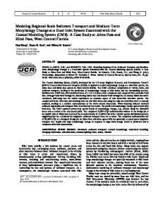
Measurement Locations

The first stretch measured, shown in figure 5.1, was from gage 1 at Myrtle Grove (River Mile 59) to Gage 2 at Pt. A La Hache (RM 48.8). The length of this stretch is 10.2 miles. The second stretch measured spanned from Gage 5 at Empire (RM 29.7) to Gage 6 at Venice (RM 10.8). Thus, the length of this stretch is 18.9 miles. From Gage 1 to Gage 2 is a shorter length than from Gage 5 to Gage 6. It is also considerably straighter than the stretch from gage 5 to Gage 6 which has two near 900 bends. The cross sectional area along the first stretch is fairly constant. The cross section remains roughly triangular with a depth of between 110 ft. and 120 ft. and a surface width of ap-

53

Stretch 1

Stretch 2

FIGURE 5.1. Stretches over which travel times were measured (yellow)

54

TABLE 5.1. Gage 1 - Gage 2 (Fluorescent Dye)

Q (cfs) tmeasured (s) tscaled 384000 30.2 420000 28 504000 21.68 624000 19.22 720000 16.25 852000 14.16 1200000 10.19 720000 16.1 624000 17.28 504000 23.32 420000 28.21 384000 29.9

(hr) U (mph) 4.50 2.27 4.17 2.44 3.23 3.16 2.87 3.56 2.42 4.21 2.11 4.83 1.52 6.71 2.40 4.25 2.58 3.96 3.48 2.93 4.21 2.43 4.46 2.29

proximately 2000 ft. at low flow. The cross section of the second section does not remain as constant. The cross sectional area at the the upper portion of the reach is very similar to the cross sectional area of the first stretch, but it changes drastically as it proceeds down river. By the end of the second stretch the river is approximately 80 ft. deep and has a roughly rectangular cross section.

5.3

Measurements

The velocity data can be seen in tables 5.1 - 5.6. Prototype data can be seen in table 5.6. These model velocites higher than those measured in the prototype coincide with the previously mentioned possibility of higher velocities causing the gradients to vary less in the model than they do in the prototype. Velocities were computed from data collected after a chemical spill in the prototype above Baton Rouge, LA on 30 May 2000. The peak concentration was measured between Baton Rouge, LA and New Orleans,LA. These data can be seen in table 5.6. Although the velocities occur at a a lower flowrate than those measured in this study, they do provide for an approximate lower bound for measured velocities. The model did produce velocities lower

55

TABLE 5.2. Gage 1 - Gage 2 (Confetti)

Q (cfs) tmeasured (s) tscaled 384000 44 420000 19 504000 28.3 624000 15.5 720000 17 852000 15 1200000 11 720000 16.5 624000 19.3 504000 25.5 420000 27.5 384000 44

(hr) U (mph) 6.56 1.55 2.83 3.60 4.22 2.41 2.31 4.41 2.53 4.02 2.24 4.56 1.64 6.22 2.46 4.15 2.88 3.954 3.80 2.68 4.10 2.49 6.56 1.55

TABLE 5.3. Gage 5 - Gage 6 (Fluorescent Dye)

Q (cfs) tmeasured (s) tscaled 384000 85 420000 79 504000 71 624000 60 720000 50 852000 41 1200000 38 720000 51 624000 58 504000 73 420000 78 384000 82

56

(hr) U (mph) 12.7 1.5 11.8 1.6 10.6 1.8 8.9 2.1 7.5 2.5 6.1 3.1 5.7 3.3 7.6 2.5 8.6 2.2 10.9 1.7 11.6 1.6 12.2 1.5

TABLE 5.4. Gage 5 - Gage 6 (Confetti)

Q (cfs) tmeasured (s) tscaled 384000 68 420000 50 504000 43 624000 39 720000 33 852000 32 1200000 23 720000 28 624000 31 504000 37 420000 40 384000 50

(hr) U (mph) 10.1 1.9 7.5 2.5 6.4 2.9 5.8 3.3 4.9 3.8 4.8 4.0 3.4 5.5 4.2 4.5 4.6 4.1 5.5 3.4 6.0 3.2 7.5 2.5

TABLE 5.5. Summary of Velocities (mph)

Q (cfs) 384000 420000 504000 624000 720000 852000 1200000 720000 624000 504000 420000 384000

Gage 1 - Gage 2 Dye Confetti 2.27 1.55 2.44 3.60 3.16 2.41 3.56 4.41 4.21 4.02 4.83 4.56 6.71 6.22 4.25 4.15 3.96 3.54 2.93 2.68 2.43 2.49 2.29 1.55

Gage 5 - Gage 6 Dye Confetti 1.49 1.86 1.60 2.54 1.79 2.95 2.11 3.25 2.54 3.84 3.09 3.96 3.34 5.51 2.49 4.53 2.19 4.09 1.74 3.43 1.63 3.17 1.55 2.54

TABLE 5.6. Prototype Values

River Mile t(Cpeak ) (hr.) U (mph) Q (1000 cfs) 232.2 7 261 175.5 31 2.4 278 154.2 40 2.4 313 104.7 63 2.2 347

57

than these, but only at the lowest flowrate. This could be a function of the values being compared being from different locations.

5.3.1

Surface V. Subsurface Velocities

The measured maximum velocity in ordinary channels usually occurs below the free surface at a distance of 0.05 to 0.25 of the depth, though the maximum velocity may often be found at the free surface (Chow 1959). Thus, the average velocity and the velocity at 0.6d are likely to be lower than the surface velocity. Moreover, for every flowrate in the prototype the velocity on the surface is greater than the velocity at 0.6d, as Chow suggested. In the second stretch, the velocities were just as Chow (1959) suggest, with the highest velocity at or near the surface. The first stretch produced more erratic results, with most surface velocities being lower, but with a few being high, and one even being the same in comparison to the dye velocities. The velocities in this stretch at the surface and below the surface are not drastically different for any of the flowrates though, suggesting that for this stretch the surface and sub-surface velocities might be approximately equal to each other. This may have to do with the shape of the channel. The shape is indicative of a scour along the north eastern bank of the river. This forces the majority of the flow to that side. Here, especially at the surface, the channel boundary appears to cause a drag effect, thus slowing down the surface velocity.

5.3.2

Model Froude Number

The SSPM’s Froude Number was calculated for each stretch at each flowrate. These values are shown in table 5.7. The number was calculated with the velocities computed in section 5.3 and average depth for the stretch. Numbers range from aproximately 0.04 at low flowrates to above 0.15 at high flowrates. these can be compared to values calculated from the average velocities for several different stages at the Carrollton gage in the prototype. This is shown in Table 5.8. The values stretch from 0.01 to 0.11, a range which contains all but the very

58

TABLE 5.7. Model Froude Number

Q (cfs) Fr (Stretch 1) Fr (Stretch 2) 384000 0.053 0.038 420000 0.057 0.028 504000 0.074 0.031 624000 0.083 0.036 720000 0.099 0.043 852000 0.113 0.052 1200000 0.157 0.056 720000 0.100 0.042 624000 0.093 0.038 504000 0.069 0.030 420000 0.057 0.028 384000 0.054 0.027

higest of the SSPM values of the Froude Number. The proximity of these values suggests Froude Number Similarity.

5.4

Sediment Time Scale

It is important to note that this applies to the hydraulic time scale, which is not the only time scale. The Sediment Time Scale is just, if not more important in our modeling. The sediment time scale, ts , it the ratio of the time it would take for sediment to pass through a certain control volume in the model to the time it would take for such an event to occur in the prototype. Our Model is based off of an empirically derived law for this developed by SOGREAH, for the Seine River estuary model as discussed in section 2.3.3. For comparison, the two rates are: E(tS ) = 0.000056

(5.2)

E(T ) = 0.001863

(5.3)

by comparing the two time scales above, one can see that the sediment movement occurs at a faster rate than the purely hydraulic properties propogate. The model was designed in this

59

TABLE 5.8. Prototype Froude Number (at Carrollton Gage)

Stage (ft.) 1 2 3 4 5 6 7 8 9 10 11 12 13 14 15 16 17 18

Fr 0.012 0.023 0.030 0.036 0.042 0.047 0.051 0.055 0.060 0.064 0.070 0.075 0.079 0.085 0.090 0.097 0.106 0.113

way to allow for sediment to accumulate at a very fast pace, as compared to the hydraulic time scale (and for that matter the prototype).

60

Chapter 6 Computer Model of SSPM area 6.1

1-D Computer Model

A computer model was developed as a complement to the physical model; many of the same features that are modeled physically in the SSPM can be modeled numerically in the computer model. Hydraulic features such as the gradients and rating curves can be computed in the computer model, along with such sediment features as bedforms and erosion/deposition. The U.S. Army Corps of Engineer’s HEC-RAS suite has the ability to model all of the quantities (Brunner, 2006). HEC-RAS stands for Hydraulic Engineering Center - River Analysis System. The HEC-RAS system contains four one-dimensional river analysis components for: 1. steady flow water surface profile computations 2. unsteady flow simulation 3. movable boundary sediment transport computations 4. water quality analysis For steady flow and quasi-unsteady (used in the sediment transport simulations), it solves one dimensional energy equation for steady and quasi-unsteady flows. The momentum equation may be used in situations where the water surface profile is rapidly varied. For unsteady flow, it solves the Saint-Venant equation using an implicit, finite difference method (Brunner, 2006). This study uses only the steady state simulations.

6.2

Geometry and Input Parameters

The geometry data that was used to construct the computer model is the same set of cartesian points that were used in the construction of the physical model. It is a combination of the

61

1992 Mississippi River Hydrographic Survey data, along with the aforementioned data from C&C Technologies. The flows are those specified for operation of the SSPM in SOGREAH and listed in table 3.4. This is also where the sediment size distribution are from. The mannings n was determined by first using values suggested by Remo and Pinter (2007) and confirmed with values suggested by Chow (1959). The expansion/contraction losses used are the HEC-RAS defaults of 0.3 and 0.1; computed WSEL did not noticably vary with an increase or decease of .05 with either of these parameters. The cross sections used for the model were on average one per mile modeled. A higher density of cross sections was placed in stretch of the river with bends and irregular or rapidly changing geometry. A lower density of cross sections was placed in the stretches that have geometry that doesnt vary greatly along the length and do not have frequent or drastic bends. The same discrete flow steps that are used in the physical model were used to model the quasi-unsteady flow for the sediment transport analysis. Levees were added on the west bank of the river down to Venice and on the east bank to the Bohemia Relief. The upsream (at Myrtle Grove) boundary condition used is a flow boundary condition for each of the flowrates listed in hydrograph described in figure 3.4. The downstream bondary condition was the rating curve listed by SOGREAH for Head of Passes. To simulate overflow into the Bohemia Relief, three diversion rating curves, that divert water based on river flowrate were added over its length. In total at maximum flowrate the model removes 200,000 cfs. The rating curve is linear from the point where no water is diverted through Bohemia Relief at a flowrate of 800,000 cfs or less.

6.3

Calibration

A steady flow analysis was conducted. Each flowrate was calibrated to the prototype by varying the mannings n value to match the Rating Curves at the gaging stations and water surface gradient of the prototype as closely as possible. The final mannings n values were

62

obtained by iterating n values within the limits provided by Chow (1959) and Remo (2006) until the the value that allowed the water surface in the model to match that of the prototype for each flowrrate as closely as possible was obtained. The initial n value tested was 0.025 and this was decreased by increments of 0.001 until the water surface of the computer model matched that of the prototype. Further reduction would have resulted in WSEL values that were drastically lower.The values for the main channel and values for the overbanks were calibrated to fine tune the WSE for different fowrates. The manning’s n for the channel was found to be n = 0.017, and for the overbanks it was found to be n = 0.018. These two values are not as different as they would normally be in when performing such modeling, but the overbank area in this model only extends accross the relatively small batture to the levee. In the area of the delta there is very little vegetation, and the river keeps the area relatively smooth. Computed gradients are shown in figures 6.1 and 6.2 at low flow and max flow respectively. The one notable problem is that stages for the gages in the upper reaches of the river are too high. The Rating curves which were used to calibrate the flowrates can be seen in figures 6.3, 6.4. Being as the downstream water surface is described by a rating curve from the prototype, it is the same in the computer model as it is in the prototype. Thus the gradient is dependent on the rating curve upstream. The rating curve at Point a La Hache can be seen in figure 6.4. The gradients produced can be seen in figure 6.1. In table 6.2 one can see a comparison of SSPM velocities to those calculated by HEC-RAS. The values for the upper stretch computed by HEC-RAS are similar to the values obtained for that stretch in the SSPM, but not to any good extent. The values for the second stretch do have a good match though. The velocities computed by HEC-RAS for this stretch are very similar to the results from the dye tests for this stretch. This is the same stretch that consistantly had confetti velocites higher than dye velocities.

63

FIGURE 6.1. Gradient as computed by HEC-RAS at 384,000 cfs

64

FIGURE 6.2. Gradient as computed by HEC-RAS at 1,200,000 cfs

65

TABLE 6.1. Comparison of Prototype, SSPM, and 1D Computer Model Gradients

Q (1000 cfs) ∇P (10−6 ) 364 3.9 384 398 6.17 407 6.52 420 444 7.14 504 580 13.0 624 720 827 15.1 852 911 15.1 1120 17.7 1150 18.3 1200

∇SSP M (10−6 )

∇RAS (10−6 )

-0.16

4.17

2.1

4.94

5.25

7.01

4.30 10.3

10.4 13.4

9.55

17.9

19.25

22.9

TABLE 6.2. Comparison of RAS and SSPM Velocities (mph)

Q (cfs) 384000 420000 504000 624000 720000 852000 1200000

Gage 1 - Gage 2 Dye RAS 2.28 1.57 2.435 1.71 3.045 2.03 2.92 2.45 4.085 2.79 4.54 3.21 6.71 4.37

66

Gage 5 - Gage 6 Dye RAS 1.52 1.47 1.62 1.60 1.77 1.91 1.82 2.32 2.37 2.65 2.79 3.07 3.34 3.49

FIGURE 6.3. Rating Curve as computed by HEC-RAS at Head of Passes

67

FIGURE 6.4. Rating Curve as computed by HEC-RAS at Pt. A La Hache

68

FIGURE 6.5. Froude Numbers as computed by HEC-RAS along the channel

69

Figure 6.5 shows Fr values for the river as computed by HEC-RAS. All values are between 0.02 and 0.10 which indicates that the HEC-RAS model has computer similar values as those obtained from the SSPM.

70

Chapter 7 Summary and Recommendations 7.1

Summary

LSU’s SSPM is a distorted vertical scale MBM intended to be used as a tool to qualitatively study the potential use of large-scale river and sediment diversions for rehabilitating and restoring some of the degraded wetlands in the Lower Mississippi River delta. The model was not designed and built for quantitative studies of the river bed morphology or detailed investigation of actual diversion structures—the model was designed to reproduce, qualitatively, the lower river sediment transport patterns under existing conditions and to evaluate various alternatives for flow and sediment diversions and new navigation channels (SOGREAH, 2003). A majority of MBMs are designed based on the relaxation of several physically-based criteria and similarity laws and through the use of lightweight sediment, a distorted vertical scale, and an increased vertical gradient in the model that results in a Fr exaggeration. Proper analysis and implementation of model results requires an understanding of these approximations and the limitations that they impose. The use of a lightweight sediment allows for the modeling of small- to medium-size sand without having to deal with cohesive forces. The SSPM utlizes a model sediment that has a specific gravity of 1.05 thus allowing for the modeling of river sands from 0.08 up to 0.25 mm. Experimental protocols have been developed to reduce the problems associated with the use of a model sediment that has a density close to that of water. The SSPM has a distorted scale of 24 which is much higher than the values recommended for detailed study of channel- or river-bed morphological processes. It should be pointed out, however, that the SSPM was not designed for this purpose. SSPM experimental re-

71

sults have demonstrated that the model is capable of qualitatively reproducing the flow and bulk sediment transport in the river and through the diversions (SOGREAH, 2003; Brown Cunningham Gannuch, 2004). The SSPM was designed using Fr similarity. One of the objectives of this thesis work was to quantitatively examine the model hydraulic gradients and to examine the ability of the model to replicate prototype water velocities. The gradients are not exactly constant along the length of the channel. As one can see in the plots in section 4.3, the gradients are generally steeper above River Mile 20 than they are below. Although the differences may be small, it is important that they are accurate as insipient motion of sediment occurs at a specific velocity, the Critical Shear Velocity. Because the sediment was scaled using the Particle Reynolds Number and the Shields Number, which are based on the Shear Velocity, it is very important that the velocities in the model scale correctly. Based on a critical analysis of the model similarity laws and scaling, a quantitative study of the model gradients and hydraulic time scales, and evaluation of model experiments, it can be concluded that the SSPM is an empirical MBM (Graf, 1971). This is primarily a result of its large vertical scale distortion and the resultant inability to quantitatively model the bed morphodynamics. However, the SSPM has been shown to be able to reproduce the prototype gradients and velocities along with the general trends in sediment transport and deposition in the river. Thus, within the context of the CCS categories, the model serves as a valuable tool as a demonstration, education and communication tool (category 1); as a screening tool to investigate the impacts of diversions on dredging within the river (category 2); a screening tool for channel and navigation alignments alternatives (category 3); and as a screening tool for environmental evaluation of modifications to the river such as side channels and notches (category 4). It is important to note that model results for studies such as these are meant to guide additional studies and are not meant to study conditions or scenarios that have the potential for endangering human life.

72

Because 1 mm in the model corresponds to 1.7 prototype feet, even small changes in the model can create results that appear to be un-physical. The resurvey work that was done as part of this thesis should serve as a guideline for monitoring the changes in base model elevations and for future re-surveys. Finally, a one-dimensional steady-state hydraulic model has been developed for the SSPM study area. The model was calibrated to actual river conditions by varying the channel and overbank Manning’s n. Proper calibration of the model at higher flowrates required the incorporation of a lateral control structure to account for the river water that exits the main river channel through the Bohemia spillway. The HEC-RAS model produced rating curves, gradients, velocities, and Froude Numbers consistent with both the prototype and the SSPM.

7.2

Recommendations

The SSPM has proven to be a very useful tool to study the potential for large-scale river flow and sediment diversions. The following recommendations are suggested in an effort to increase the usefulness of the model: 1. Re-surveying of the BMELs should be made on a regular basis. 2. Carefully conducted gradient and velocity measurements should be made on a regular basis as they are vital to re-validate the similarity laws. 3. Recently acquired high precision pressure transducers should be installed in the model. One can be used to provide more proactive monitoring and adjustment of sea level while the second can be used to measure the WSEL above Myrtle Grove. These can provide very accurate water surface gradients 4. Recently acquired micro-Acoustic Doppler Velocimeters (micro-ADVs) should be used for high precision velocity measurements. This can be used to ensure Froude Numbers stay within proper ranges

73

5. The HEC-RAS model should be extended to study the transient response to each of the river flow diversion scenarios that have been tested. This could provide valuable information for navigation interests. 6. The HEC-RAS model should also be extended to study sediment transport in the SSPM area. Of particular interest would be: (1) a comparison to the SSPM results concerning depositional areas which impact dredging; and (2) potential shoaling in regions around the diversion structures. 7. The HEC-RAS model should be calibrated to the SSPM WSEL data to determine the manning’s n in the SSPM.

74

References Andrus, T. M. (2007). “Sediment flux and fate in the mississippi river diversion at west bay: Observation study. Master’s thesis, Louisiana State University and Agricultural and Mechanical College. Brown Cunningham Gannuch, C. R. C. (2004). “Report on the feasibility of a small-scale physical model of the lower mississippi river delta for testing water and sediment diversion projects.” Report no., Louisiana State University. Brunner, G. W. (November 2006). HEC-RAS, River Analysis System User’s Manual. 609 Second Street, Davis, CA 95616-4687. Chow, V. T. (1959). Open Channel Hydraulics. McGraw-Hill, New York, NY. CREST (2006). “On Reintroducing Riverine Processes in the Mississippi Delta Region. http://www.gulfcrest.org/docs/Diversions Day, John W., J., Pont, D., Hensel, P. F., and Ibanez, C. (1995). “Impacts of Sea-Level Rise on Deltas in the Gulf of Mexico and the Mediterranean: The Importance of Pulsing Events to Sustainability.” Estuaries, 18, 636–647. Dill, N. L. (2007). “Hydrodynamic Modeling of a Hypothetical River Diversion Near Empire, Louisiana. Master’s thesis, Louisiana State University and Agricultural and Mechanical College. Ettema, R., Arndt, R., Roberts, P., and Wahl, T. (2000). Hydraulic Modeling: Concepts and Practice. ASCE. Fischer, H. B., List, J. E., Koh, C. R., Imberger, J., and Brooks, N. H. (1979). Mixing in Inland and Coastal Waters. Academic Press. Graf, W. H. (1971). Hydraulics of sediment transport. McGraw-Hill, New York, NY. Kundu, P. K. and Cohen, I. M. (2004). Fluid Mechanics. Academic Press, New York, NY. Maynord, S. (2006). “Evaluation of the micromodel: An extremely small-scale movable bed model.” Journal of Hydraulic Engineering, 132(4), 343–353. Miller, G. (2004). “Mississippi River – West Bay Sediment Diversion.” Critical Transitions in Water and Environmental Resources Management - proceedings from he 2004 World Water and Environmental Resources Congress: June 27 – July 1, 2004, Salt Lake City, UT, ASCE, Reston, VA. Mossa, J. (1996). “Sediment dynamics of the lowermost mississippi river.” Engineering Geology, 45, 457–479.

75

Reed, D. J. (1989). “Patterns of sediment deposition is subsiding coastal salt marshes, terrebonne bay, louisiana: the role of winter storms.” Estuaries, 12, 222–227. Remo, J. and Pinter, N. (2007). “Retro modeling the Middle Mississippi River.” Journal of Hydrology, 421–435. Singh, V. (1991). Elementary Hydrology. Prentice Hall, Upper Saddle River, NJ. SOGREAH (2003). “Small-scale physical model of the mississippi delta. U.S. Army Corps of Engineers (2004). “Rep. on the 68th Meeting, Micromodeling. Willson, C., Dill, N., Bartlett, W., Danchuk, S., and Waldron, R. (2007). “Physical and Numerical Modeling of River and Sediment Diversions in the Lower Mississippi River Delta.” ASCE Coastal Sediments, New Orleans, Louisiana, USA. 749–761.

76

Vita Ryan L. Waldron was born in September of 1983, in New Orleans, LA. He finished his Bachelors of Science at Tulane University in December 2005. In January 2006, after having already spent one semester at Louisiana State University due to Hurricane Katrina, he began to pursue graduate studies in civil engineering. He is currently a candidate for the degree of Master of Science in Civil Engineering, which will be awarded in May 2008.

77