Physical Realization of Generic-Element Parameters in ... - CiteSeerX

H. Ahmadian Department of Mechanical Engineering, Iran University of Science and Technology, Tehran 16844, Iran e-mail:[email protected]

J. E. Mottershead Department of Engineering, Mechanical Engineering Division, The University of Liverpool, Liverpool L69 3GH, UK e-mail:[email protected]

M. I. Friswell Department of Mechanical Engineering, University of Wales Swansea, Swansea SA2 8PP, UK e-mail:[email protected]

1

Physical Realization of Generic-Element Parameters in Model Updating The selection of parameters is most important to successful updating of finite element models. When the parameters are chosen on the basis of engineering understanding the model predictions are brought into agreement with experimental observations, and the behavior of the structure, even when differently configured, can be determined with confidence. Physical phenomena may be misrepresented in the original model, or may be absent altogether. In any case the updated model should represent an improved physical understanding of the structure and not simply consist of unrepresentative numbers which happen to cause the results of the model to agree with particular test data. The present paper introduces a systematic approach for the selection and physical realization of updated terms. In the realization process, the discrete equilibrium equation formed by mass, and stiffness matrices is converted to a continuous form at each node. By comparing the resulting differential equation with governing equations known to represent physical phenomena, the updated terms and their physical effects can be recognized. The approach is demonstrated by an experimental example. 关DOI: 10.1115/1.1505028兴

Introduction

Finite element model updating 关1,2兴 is employed to bring the predictions of the model into agreement with experimental observations from a physical structure. This can be achieved provided that the measured data represent the actual behavior of the structure and are not contaminated to an unacceptable level with random or systematic errors. In the presence of good quality test data updating procedures should be focused on the sources of discrepancies between the test and the finite element model. They should locate the areas that are mismodelled and provide a more accurate model for them. The accuracy of the updated model depends upon the parameters chosen for updating. The predictions should be sensitive to the chosen parameters, but the parameters themselves must be able to define the phenomena that was either mismodelled or not present in the initial model. There are basically two parameter selection strategies in the literature. A discussion that includes the performance of the different approaches can be found in 关3兴. One approach is to select the geometric or material input data of the finite element model and by modifying them improve the correlation between the model predictions and the experiment. The modification can be performed on individual or selected groups of elements. The method is very popular due to the fact that it can be implemented in existing finite element codes and more importantly, because there is a readily available physical explanation for each modified term. However the method is incapable of changing the mathematical ‘‘structure’’ of the model, so that structural mismodelling and omitted effects cannot be corrected. Errors of this type include the omission of shear effects, stress stiffening and coupling of bending and torsion in beams. The second strategy, in a contrast to the first, allows changes in all entries of the system matrices 共or a subset of them兲. The method allows the updated model to reproduce observed behavior exactly, but there is no guarantee that it represents a physical system and not a meaningless numerical expression that reproduces the test data. A common problem is the loss of positivity of system matrices. The updated matrices may be indefinite and not 共semi-兲positive definite as required, whereas in the first approach Contributed by the Technical Committee on Vibration and Sound for publication in the JOURNAL OF VIBRATION AND ACOUSTICS. Manuscript received December 2000; revised February 2002. Associate Editor: C. R. Farrar.

628 Õ Vol. 124, OCTOBER 2002

the definiteness properties remain unchanged when the parameters are varied over a wide range 共for example all positive values of Young’s modulus兲. The definiteness of the model can be preserved by introducing the rigid body modes of the structure into the updating process. This idea was applied at the element level by assuming the initial model had the correct connectivity pattern and led to the concept of generic elements 关4,5兴. A genericelement model is a parametric form of the element matrices that provides for a family of all allowable models of that element. Despite many advances, the second strategy cannot always be used with complete confidence. In many cases a physical explanation of the modified terms is not readily available. The updated model should be able to predict the behavior of the structure in loading and support conditions other than those in the test. A physical explanation of the updated terms ensures that the modifications are not just numerical values that match the test results but are justified by engineering understanding of the system and the test carried out on it. In this article we begin by defining what we mean by generic elements. In the original work 关4,5兴 parameters were defined in the modal domain using eigenvalues and eigenvectors of the initial model at the element level. But, a physical explanation of updated terms in the modal domain of an element is not always available. Here a systematic approach is introduced to explain the physical meaning of changes occurring in updated generic elements when they are defined in the spatial domain. The approach is to reduce the number of parameters to be identified by the application of constraints including matrix symmetry, invariance of the element matrices to rotation 共where applicable兲, and the application of the rigid-body modes to define the null-space of element stiffness matrices and the principal mass and inertia properties of element mass matrices. A further constraint, that the internal forces at the nodes should zero, is introduced for the first time in the definition of generic elements. A finite element model defines the dynamic equilibrium condition of the physical structure in a discrete form. The updated model also defines the same equilibrium conditions taking into account mismodelled and neglected effects. The discrete updated equations can be converted to continuous form. In this paper the conversion is achieved using Taylor series expansion of displacements at different finite element nodes in terms of the displacement of a reference node. Having determined the continuous gov-

Copyright © 2002 by ASME

Transactions of the ASME

erning equations from an updated model, one may realize the physical significance of added terms in the updating procedure. A case study is performed to demonstrate the physical realization of an updated model.

2

1 关 ⫺k j k j ⫹k j⫹1 ⫺k j⫹1 兴 L

冋

⫹L m j ␤ 共 m j ⫹m j⫹1 兲

The Generic-Element Model

The updating of a finite element model is performed with a limited amount of experimental data from the structure. Inevitably an analyst must make some assumptions about the nature of mismodelled or neglected effects in order to improve the chance of tracing them successfully in updating. The basic assumption in every updating procedure is that the order and the structure of the finite element model is correct. In other words, the structure of the initial model is capable of accommodating all the physical effects that are somehow represented in the measured data. We begin with this assumption and define generic parameters for each element of the initial finite element model. This approach is special because it permits neglected effects to be included so that the physical meaning of the model is improved when updated. Modification of a finite element model at the element level implies confidence in the connectivity of initial model. When this is in doubt a generic model of the group of elements that include the doubtful connectivity may be constructed. Reference 关6兴 uses a generic model for a branched joint represented by three beam elements in an initial model. A generic element model is built by imposing all necessary conditions that the element must satisfy: the element mass matrix M is positive definite, and its stiffness matrix K is semi-positive definite. The rigid body modes of element ⌽R span the null space of the stiffness matrix and are related to the mass matrix as, K⌽R ⫽0,

⌽RT M⌽R ⫽

冋 册 m 0

J

K⫽

冋

k L ⫺1

1

册

,

M⫽mL

冋

␤

␤

1 2⫺␤

册

k⬎0, ,

␤ ⬍ 41

(2)

where k is the axial stiffness, m is mass per unit length, and L is the length of the element. The form of the matrices is determined only by Eqs. 共1兲, uniformity and symmetry. The condition ␤ ⬍ 41 arises from the positive definiteness requirement on the mass matrix. It can be seen that ␤ produces different possible mass matrices for the bar element: ␤ ⫽0 produces a lumped mass matrix. ␤ ⫽ 61 corresponds to a consistent mass matrix with linear shape functions, ␤ ⫽ 81 creates a consistent mass matrix with harmonic 1 shape functions and ␤ ⫽ 12 produces a mass matrix with minimum discritization error for a uniform bar. The parameters of each element may vary independently during updating. We may, however, introduce more constraints on the parameters by insisting that inter-element forces are in equilibrium. We develop the equation of motion using generic models and then apply the requirement of equilibrium on the interelement forces. The following example demonstrates the procedure. Consider part of a structure modelled using bar elements. We select a row of the free vibration equation which consists of nodes i⫺1, i, i⫹1 corresponding to bar elements j and j⫹1 with equal length of L and different physical properties, Journal of Vibration and Acoustics

册再

冎

u¨ i⫺1 u¨ i ⫽0. u¨ i⫹1

The displacements at nodes i⫺1, and i⫹1 can be defined in terms of u i and its derivatives using the Taylor series expansion, ⬁

u i⫺1 ⫽u i ⫹

共 ⫺1 兲 n ⳵ n u i n L , n! ⳵xn

兺

n⫽1

⬁

u i⫹1 ⫽u i ⫹

兺

n⫽1

1 ⳵ nu i n L . n! ⳵ x n (4)

By substituting these values into Eq. 共3兲, we obtain a series of continuous differential equations, ⬁

⫺

k j⫹1 ⫹ 共 ⫺1 兲 n k j ⳵ n u i n L 2 L ⫹ 共 m j ⫹m j⫹1 兲 u¨ i n! ⳵xn 2

兺

n⫽1

⬁

⫹␤

兺

n⫽1

m j⫹1 ⫹ 共 ⫺1 兲 n m j ⳵ n u¨ i n⫹2 L ⫽0. n! ⳵xn

(5)

The expression obtained for the equation of motion contains different orders of L. The element length is an independent parameter therefore the right hand side of the equation of motion is zero only if each order is equal to zero independently. The first order terms,

(1)

2.1 Bar Element. The generic element for a uniform bar can be expressed in the form, ⫺1

1 ⫺ ␤ m j⫹1 ␤ 2

L 1 ⇒⫺ 共 k j⫹1 ⫺k j 兲

where in general m is a diagonal 3⫻3 matrix with the total mass of the element as its nonzero entries and J is the 3⫻3 inertia products matrix. A generic element model is developed by imposing the above necessary conditions on the element matrices. The meaning of generic-element parameters is now explained by means of bar and beam examples.

1

冉 冊

(3)

0

1 2⫺␤

再 冎 u i⫺1 ui u i⫹1

⳵ui ⳵x

(6)

define the sum of internal forces at node i and must be zero even when the adjacent element have different properties. It seems, however, that this cannot be achieved without setting ⳵ u i / ⳵ x ⫽0. The difficulty can be removed by assuming a linear relationship between the element parameters and the physical properties of the rod at the element nodes, k j⫹1 ⫽c 1 k i ⫹c 2 k i⫹1 , m j⫹1 ⫽c 3 m i ⫹c 4 m i⫹1 ,

k j ⫽c 1 k i⫺1 ⫹c 2 k i , m j ⫽c 3 m i⫺1 ⫹c 4 m i

(7)

where k i and m i are axial stiffness and mass per unit length of the rod at node i. We substitute Eq. 共7兲 into 共5兲 and expand k i⫾1 ⫽k i ⫾L ⳵ k i / ⳵ x, m i⫾1 ⫽m i ⫾L ⳵ m i / ⳵ x. The result sorted in orders of L is, L 1 ⇒ 共共 c 1 ⫹c 2 兲 ⫺ 共 c 1 ⫹c 2 兲兲 k i L 2 ⇒⫺ 共 c 1 ⫹c 2 兲 L 3⇒

⳵ui ⫽0, ⳵x

冉 冊 冉 冊

⳵ ⳵ui ki ⫹ 共 c 3 ⫹c 4 兲 m i u¨ i ⫽0, ⳵x ⳵x

(8)

⳵ ⳵ki ⳵ui ⳵mi 1 1 ¨u ⫽0. ⫺ 共 c 3 ⫺c 4 兲 共 c 1 ⫺c 2 兲 2 ⳵x ⳵x ⳵x 2 ⳵x i

The first of Eqs. 共8兲 is satisfied automatically. If we consider the uniform bar for which c l ⫽1/2, l⫽1, . . . ,4, then we see that the second and third-order terms go to zero and the fourth order terms appear as, L 4 ⇒⫺

1 ⳵ 4u i 1 ⳵ k i ⳵ 3u i 1 ⳵ 2k i ⳵ 2u i 1 ⳵ 3k i ⳵ u i k ⫺ ⫺ ⫺ 12 i ⳵ x 4 6 ⳵ x ⳵ x 3 4 ⳵ x 2 ⳵ x 2 6 ⳵ x 3 ⳵ x

冉

⫹␤ mi

冊

⳵ 2 u¨ i ⳵ m i ⳵ u¨ i ⳵ 2 m i ⫹ ⫹ ¨u ⫽0. ⳵x2 ⳵x ⳵x ⳵x2 i

(9)

OCTOBER 2002, Vol. 124 Õ 629

Inspection of Eq. 共9兲 showed that fourth order terms in the equation of motion of a bar element cannot be set to zero unless k i , m i 1 are constant and ␤ ⫽ 12 . In that case the fourth order terms lead to the expression,

冉

冊

⳵2 ⳵ 2u i ⫹m i u¨ i ⫽0, 2 ⫺k i ⳵x ⳵x2

(10)

from which we recognize the differential equation governing axial deflection in a uniform rod. The equilibrium constraint on internal forces at each node defines relationships for the generic parameters that may be used in updating. In the case of the beam element the number of parameters is reduced when these constraints are applied. 2.2 Beam Element. A generic beam element with nodes i and i⫹1, and degrees of freedom 关 w i ,L ␪ i ,w i⫹1 ,L ␪ i⫹1 兴 T has the following general form for the stiffness matrix,

K⫽

冋

k ww

k w␪

⫺k ww

k ww ⫺k w ␪

k w␪

k ␪␪

⫺k w ␪

k w ␪ ⫺k ␪␪

⫺k ww

⫺k w ␪

k ww

⫺k ww ⫹k w ␪

k ww ⫺k w ␪

k w ␪ ⫺k ␪␪

⫺k ww ⫹k w ␪

k ww ⫹k ␪␪ ⫺2k w ␪

k ww ⬎0,

k ␪␪ ⬎0,

kwwk␪␪⬎kw2 ␪.

册

冉

冊

(11)

(12)

3 ⳵ k i⫹1 3 ⳵ki L⫺ L, 5 ⳵x 5 ⳵x

1 ⳵ k i⫹1 21 9 2 ⳵ki k w ␪ ⫽ k i ⫹ k i⫹1 ⫹ L⫺ L, 5 5 5 ⳵x 5 ⳵x

(13)

2 ⳵ k i⫹1 16 4 1 ⳵ki k ␪␪ ⫽ k i ⫹ k i⫹1 ⫹ L⫺ L. 5 5 3 ⳵x 15 ⳵ x

2.3 Geometric Symmetry. Further restrictions can be imposed on an element if it has symmetry axes. In that case the invariance of the matrix entries to rotation of the element about one or more of the axes of symmetry is used to further reduce the number of unknown parameters. The constraint can be expressed in the form, M⫽RT MR

630 Õ Vol. 124, OCTOBER 2002

1 L3

冋

k ww

,

R⫽

冋

0

0

1

0

0 1

0

0

⫺1

0

0

0

0

⫺1

0

0

k ww /2

⫺k ww

k ww/2

k ␪␪

⫺k ww /2

k ww /2⫺k ␪␪

k ww

⫺k ww /2

Sym.

M⫽ ␳ AL

冋

k ␪␪

(14)

m 11

m 12 m 22

1 2

⫺m 11

m 14

⫺m 14

m 24

m 11

⫺m 12

Sym.

m 22

册

1 m 11 m 24⫽ ⫺ ⫹m 12⫹m 14⫺m 22 , 6 2

册

册

(15)

,

(16)

,

(17)

where the stiffness matrix has two independent parameters k ww , k ␪␪ and the mass matrix is formed using four independent parameters, m 11 , m 12 , m 14 , m 22 . The generic model constructed for a symmetric beam element is capable of representing all possible effects in a symmetric element: the choice of k ww ⫽12EI, k ␪␪ ⫽4EI and m 11⫽13/35, m 12⫽11/210, m 14⫽13/420, m 22⫽1/105 creates a uniform Euler-Bernoulli beam model with a consistent mass matrix obtained from cubic shape functions. A more accurate model for dynamic analysis of the Euler-Bernoulli beam is formed if we set m 11⫽163/420, m 12⫽51/840, m 14⫽⫺19/840, m 22 ⫽15/840. It may be shown that the latter mass matrix results in discretization errors of the 6th order while the consistent mass matrix has 4th order errors 关7兴. A Timoshenko beam element including shear effects is obtained by selecting, k ww ⫽EI

m 11⫽

It is clear from the above that we may relate the 3 genericelement stiffness parameters to 2 parameters at the nodes, namely k i and ⳵ k i / ⳵ x, and hence reduce the number of parameters. For example if a beam is modeled with N elements, the number of parameters can be reduced from 3⫻N to 2⫻N⫹2. The obtained generic stiffness matrix gives the most accurate form to define an Euler-Bernoulli beam with variable cross section.

K⫽RT KR,

which implies,

K⫽

w2 ⫺L ␪ 2 w1 ⫺L ␪ 1

⫽R

,

and minimizing the error up to the sixth order terms restricts an element with nodes i and i⫹1 to have parameters of the following form, k ww ⫽6k i ⫹6k i⫹1 ⫹

再冎再 冎 w1 L␪1 w2 L␪2

k ␪␪ ⬎k ww /4⬎0,

The above generic stiffness model can accommodate any effect that is defined using the specified degrees of freedom. Restricting the model to Euler-Bernoulli beam theory and applying equilibrium constraints on the internal moments and shear forces one can reduce the number of generic parameters by relating k ww , k w ␪ and k ␪␪ of each element to the nodal bending stiffness k i and its first derivative ⳵ k i / ⳵ x. The result of satisfying the requirement that internal forces are in equilibrium, to the fourth order, is the governing equation of,

⳵2 ⳵ 2w i k ⫹m i w¨ i ⫽0 i ⳵x2 ⳵x2

where the matrix R is a transformation matrix which relates the element coordinates before and after rotation. In the case of a symmetric beam element with nodes 1 and 2, the rotation matrix is developed from the identity,

m 12⫽

冉 冉

k ␪␪ ⫽EI

13 7 1 ⫹ g⫹ g 2 35 10 3

冊冒 冊冒 冊冒 冊冒

4⫹g 1⫹g

共 1⫹g 兲 2

11 11 1 ⫹ g⫹ g 2 210 120 24

共 1⫹g 兲 2

冉

13 3 1 ⫹ g⫹ g 2 420 40 24

共 1⫹g 兲 2

1 1 1 2 ⫹ g⫹ g 105 60 120

共 1⫹g 兲 2

m 14⫽⫺

m 22⫽

冉

12 1⫹g

g⫽

CEI GAL 2

(18)

where C is the cross section shape factor. Also a beam element with a crack at half its length may be formed by assigning, Transactions of the ASME

k ww ⫽ k ␪␪ ⫽

12EI , 1⫹ 共 1⫺ ␯ 2 兲 ␣ 3 F 2

EI 关 4⫹ 共 1⫺ ␯ 2 兲共 18␣ F 1 ⫹2 ␣ 3 F 2 兲兴 关 1⫹6 共 1⫺ ␯ 2 兲 ␣ F 1 兴关 1⫹2 共 1⫺ ␯ 2 兲 ␣ 3 F 2 兴

(19)

where ␣ ⫽h/L is the ratio between the thickness and the length of the element and the functions,

F 1⫽

冕

a/h

0

and, F 2⫽

冕

a/h

0

2 tan

冉 冊冉 冉 冉 冊冊 冉 冊 ␲s 2

0.199 1⫺sin cos2

␲s 2

⫹0.923

␲s 2

冊

2

ds (20)

␲s2 共 3⫺2s 兲 2 共 1.122⫺0.561s⫹0.085s 2 ⫹0.18s 3 兲 2 ds 1⫺s (21)

are products of stress intensity factors for opening type and sliding type cracks respectively 关8兴, and a is the crack depth. We consider the case where the element thickness is small compared to its length and take into account only the first order terms in ␣. Then the formulation of a cracked beam is simplified to, k ww ⫽12EI,

k ␪␪ ⫽EI 共 4⫺6 共 1⫺ ␯ 2 兲 ␣ F 1 兲 .

(22)

This means that in the resulting finite element formulation of the cracked beam the crack is modelled as a lumped bending spring with a negative constant. We have shown that by a generic element approach a small set of parameters may be found for updating by satisfying a variety of constraints including null-space requirements, equilibrium of internal forces and moments, and element symmetry. In the case of plate, shell, solid or other elements satisfying the equilibrium of internal forces at nodes the number of parameters may again be reduced significantly 关9兴. The next section deals with the challenge of determining the physical meaning of an updated model using the parameterization described above.

3

Physical Realization of Parameters

Processing updated models is the most important step in understanding the dynamical behavior of a structure. By realization of the modified terms one finds those characteristics of the test structure that were not included in the initial model. However the task of realization of the physical meaning of each modified term is not straightforward and is mainly based on the engineering judgment of the analyst. For example, we would like to find out if a change is due to the shear effect, stress stiffening, or a local crack, etc. It is shown in the previous section that all these effects can be accounted for by changes in a similar set of parameters. It is demonstrated how physical phenomena attributed to the discrepancies between experimental data and the prediction of an initial model can be extracted from modified terms in an updated model. In modelling a continuous structure using the finite element method a discrete model of a bar, beam, shell, or solid is assigned to each element. When the generic model of each element exhibits its true nature then the updated model represents a discrete version of the equation of motion of the physical structure. At each element the discrete equation can be converted to a continuous form as demonstrated in Eqs. 共3兲–共5兲 and compared with existing continuous models to find the effect it represents. The method is demonstrated using the following updating exercise. The experimentally measured modes of a simply supported uniform steel beam with the length 575 mm and of rectangular cross section 31.75 mm depth and 9.525 mm breadth with a symmetric crack at mid-span are reported by Christides and Bar 关10兴 and Shen and Pierre 关11兴. Christides and Bar presented a onedimensional theory of the cracked Euler-Bernoulli beam and veriJournal of Vibration and Acoustics

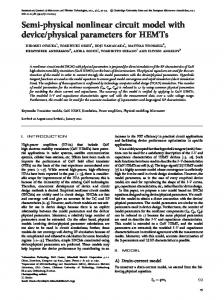
Fig. 1 Changes in lateral stiffness

fied their predictions by the experimentally measured first natural frequency of the beam with different crack sizes. Shen and Pierre presented a solution to obtain the mode shapes and natural frequencies of the cracked beam based on the Christides and Bar theory. They verified their method using the experimentally measured natural frequencies and predictions of finite element models of the cracked beam developed using rectangular and triangular plate elements. We use the first experimentally measured natural frequency and corresponding mode shape to update the initial finite element model which is formed using uniform EulerBernoulli beam elements with no crack effect introduced. The case where the first mode is reduced to 0.76% of its initial value after introducing the crack is used in updating. The aim is to update the model and find a physical justification, i.e. location and the size of the crack, for the updated terms. Parameterizing a crack by using a lumped rotational spring is established in the literature. It was shown earlier that one formulation of a cracked beam element effectively models a crack as a lumped rotational spring with a negative stiffness of k ␪ ⫽⫺6EI(1⫺ ␯ 2 ) ␣ F 1 . However such a lumped model produces accurate results only for one mode and cannot predict the behavior of the structure over a wide frequency range. Moreover the zone affected by a crack in a lumped model has zero length while in reality the stiffness of the beam is affected over a finite region local to the crack. Our purpose is to develop an updated model not limited by the restrictions of the negative lumped spring, and therefore we start with the generic form of the beam element stiffness developed in Eq. 共11兲. There are 3 parameters in each element to be updated, namely k ww , k w ␪ , and k ␪␪ . We may update the beam model using these three parameters in each element. However by using only the first mode of a thin beam in updating we may neglect the shear effects and assume that the Euler-Bernoulli model defines the characteristics of the structure adequately. This reduces the number of parameters to two per node by insisting on the equilibrium of inter-element forces of a beam described in the previous section, i.e., we select k i and ⳵ k i / ⳵ x as updating parameters. An equation error function is formed using the first mode. The equations are weighted based on the strain energy of the related areas to avoid large changes in parameters that do not contribute to the strain energy of the first mode. The updating was performed with different numbers of elements to ensure the stability of the results. The updating results, i.e., the percentage change in parameters k i and ⳵ k i / ⳵ x are shown in Figs. 1 and 2. As expected, a sharp reduction in stiffness at the center of the beam is predicted. We might attempt to further reduce the number of updating parameters, and for the purpose of illustration the updating was OCTOBER 2002, Vol. 124 Õ 631

Fig. 2 First derivative of the lateral stiffness

Fig. 4 Constant element properties

carried out again using two different sets of parameters. In the first it is assumed k i varies linearly along the element, i.e., ⳵ k i⫹1 / ⳵ x ⫽ ⳵ k i / ⳵ x and higher derivatives of k i are zero. Therefore the element parameters can be defined using k i and k i⫹1 as,

the first order in L. The two cases considered demonstrate the need for both of the parameters k i and ⳵ k i / ⳵ x when updating the cracked beam. We have obtained reliable results from updating k i and ⳵ k i / ⳵ x and the remaining task is to find the associated physical meaning of the updated terms. To find the physical meaning we form the governing equation of the beam at each node using the updated model. The governing equation for a generic beam model with variables k i , ⳵ k i / ⳵ x is represented in Eq. 共12兲. The obtained governing equation suggests a beam with variable bending flexibility. Christides and Barr 关10兴 developed a one-dimensional theory of the cracked Euler-Bernoulli beam by defining the governing equation,

k w␪⫽

冉 冉

k ww ⫽6k i ⫹6k i⫹1 ,

冊 冊

21 9 1 ⳵ki ⳵ki k⫹ L ⫹ L⫽4k i ⫹2k i⫹1 , k⫹ 5 i 5 i ⳵x 5 ⳵x

k ␪␪ ⫽

(23)

16 4 1 ⳵ki ⳵ki k i⫹ k i⫹ L ⫹ L⫽3k i ⫹k i⫹1 . 5 5 ⳵x 5 ⳵x

The results of updating assuming a linear variation of beam properties are shown in Fig. 3. In the second case k i is assumed constant within the element i.e. k ww ⫽12k i , k w ␪ ⫽6k i , k ␪␪ ⫽4k i , and the results are shown in Fig. 4. The results of modifying k i from both latter methods are similar to each other but are different from the results when both k i and ⳵ k i / ⳵ x are updated. The observations were verified using different numbers of elements. This can be simply explained by the fact that the selection of ⳵ k i / ⳵ x as a constant or zero along the element results in a zero order estimation of the parameters. In these cases the sum of the internal forces at each node is not zero and the estimate contains errors of

冉

632 Õ Vol. 124, OCTOBER 2002

(24)

where Q(x) is the crack disturbance function defined as,

冋 冉冉 冊 冊 冉 冏 冏 冊 册

Q 共 x 兲 ⫽ 1⫹

h h⫺a

3

⫺1 EX P ⫺2 ␥

x⫺x c h

⫺1

(25)

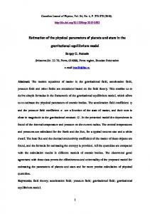
where as before h is the beam thickness, a is size of the crack and x c is location of the crack. Christides and Barr used the constant ␥ to specify the area affected by the crack and evaluated it from experimental observation. Later Shen and Pierre 关11兴 showed that for symmetric cracks ␥ is independent of the location or size of a symmetric crack and is equal to 1.936. Realization of updated parameters is performed by comparing the governing equation of the updated model at each node with the proposed governing equation of Christides and Barr. The change in k i at each node is equal to the value of 1⫺Q(x) evaluated at that node. We evaluated the crack size by comparing Q i ⫽1⫹⌬k/k 0 at each node with Q(x) and found a/h⬇ 32 which is consistent with the test report 关10兴. Figure 5 shows the identified 2 Q i at each node and the values of Q(x) for a/h⫽ 3 . Constructing the governing equation of the beam from the updated model enabled us to find a physical explanation for the change in each parameter.

4

Fig. 3 Linearly varying element properties

冊

⳵2 ⳵ 2w EIQ x ⫹ ␳ Aw ¨ ⫽0 兲 共 ⳵x2 ⳵x2

Conclusions

Generic element models for updating are developed by constraining the model to have the appropriate null space, positivity properties, total mass and moments of inertia and geometric symmetry 共if appropriate兲. The parameters are also constrained to meet the requirements of internal-force equilibrium at each node. The generic-element models obtained by this approach can be Transactions of the ASME

Acknowledgment The research was supported by grant GR/N16334 from the Engineering and Physical Sciences Research Council.

References

Fig. 5 Disturbance function—exact „solid…, identified „circled…

used in model updating. The physical meaning of the updated terms are not always readily available but may be explained by the governing differential equation produced at each node after updating. The governing equation produced by the method can be compared to existing governing equations in the literature to establish the physical meaning for the updated terms. The procedure of parameterization and physical realization is demonstrated by updating a model using experimental data obtained from a cracked beam.

Journal of Vibration and Acoustics

关1兴 Mottershead, J. E., and Friswell, M. I., 1993, ‘‘Model Updating in Structural Dynamics: A Survey,’’ J. Sound Vib., 162共2兲, pp. 347–375. 关2兴 Friswell, M. I., and Mottershead. J. E., 1995, Finite Element Model Updating in Structural Dynamics, Kluwer Academic Publisher, Dordrecht. 关3兴 Ahmadian, H., Gladwell, G. M. L., and Ismail, F., 1997, ‘‘Parameter Selection Strategies in Finite Element Model Updating,’’ ASME J. Vibr. Acoust., 119共1兲, pp. 37– 45. 关4兴 Ahmadian, H., 1994, ‘‘Finite Element Model Updating Using Modal Testing Data,’’ Ph.D. thesis, University of Waterloo, Canada. 关5兴 Gladwell, G. M. L., and Ahmadian, H., 1995, ‘‘Generic Element Matrices Suitable for Finite Element Model Updating.’’ Mech. Syst. Signal Process., 9共6兲, pp. 601– 614. 关6兴 Ahmadian, H., Mottershead, J. E., and Friswell, M. I., 1996, ‘‘Joint Models for Finite Element Model Updating,’’ 14th International Modal Analysis Conference, Dearborn, February, pp. 591–596. 关7兴 Stavrinidis, C., Clinckemaillie, J., and Dubois, J., 1989, ‘‘New Concept for the Finite Element Mass Matrix Formulations.’’ AIAA J., 27共9兲, pp. 1249–1255. 关8兴 Qian, G.-L., Gu, S.-N., and Jiang, J.-S., 1990, ‘‘The Dynamic Behavior and Crack Detection of a Beam With a Crack.’’ J. Sound Vib., 138共2兲, pp. 233– 243. 关9兴 Ahmadian, H., Friswell, M. I., and Mottershead, J. E., 1998, ‘‘Minimization of the Discretization Error in Mass and Stiffness Formulation by an Inverse Method,’’ Int. J. Numer. Methods Eng., 41, pp. 371–387. 关10兴 Christides, S., and Barr, A. D. S., 1984, ‘‘One Dimensional Theory of Cracked Bernoulli-Euler Beams.’’ Int. J. Mech. Sci., 26共11/12兲, pp. 639– 648. 关11兴 Shen, M.-H. H., and Pierre, C., 1990, ‘‘Natural Modes of Bernoulli-Euler Beams with Symmetric Cracks,’’ J. Sound Vib., 138共1兲, pp. 115–134.

OCTOBER 2002, Vol. 124 Õ 633