Physics-Based Reliability Assessment of a Heat Exchanger Shell

AMO - Advanced Modeling and Optimization, Volume 13, Number 3, 2011*

Physics-Based Reliability Assessment of a Heat Exchanger Shell O.M. Al-Habahbeh1, D.K. Aidun2, and P. Marzocca3 1

Mechatronic Engineering Dept., The University of Jordan, Amman, 11942 Jordan

2&3

Mechanical & Aeronautical Eng. Dept., Clarkson University, PO Box 5725, Potsdam, NY 13699 USA 1

Corresponding author, [email protected], Tel: +962787156824, Fax: +96265300813 2

[email protected], 3 [email protected]

Abstract: A novel physics-based stochastic method is employed to estimate the reliability of a heat exchanger shell. This component is part of an energy conversion system. In order to perform the reliability assessment task, several computational tools are integrated. These tools include Computational Fluid Dynamics (CFD), Finite Element Method (FEM), Fatigue analysis, and Monte Carlo Simulation (MCS). The method starts with CFD analysis to determine the heat transfer parameters needed for the transient FEM thermal analysis. The FEM analysis provides maximum thermal stress whereby the fatigue life of the component is estimated. As a result of input parameters randomness, the resulting life will be in the form of a Probability Density Function (PDF), which enables the computation of the reliability of the component. The application of this reliability assessment method to the heat exchanger shell can be used to enhance the design and operation of the component by revealing under-design or over-design. Under-design warrants further investigations in order to determine how to enhance the reliability. On the other hand, over-design should be eliminated in order to minimize the manufacturing cost of the component. Furthermore, this method enables the study of alternative designs and operational scenarios as it depends on parametric modeling. Keywords: Integrated Reliability Assessment, CFD Simulation, Heat exchanger shell, Finite element methods, Thermal stresses, Lifetime estimation, Monte Carlo methods

1. Introduction Reliability can be defined as the ability of a system to perform certain tasks for a specific life time. The system should operate under normal and abnormal conditions subject to a defined failure rate [Yang, 2007]. While accelerated-life testing could be used to estimate the reliability of a component, it is more cost-effective to predict the reliability early during the design phase. Research on reliability has gone a long way. However, most of the previous work is related to structural systems not involving fluid interaction. Basaran and Chandaroy determined the reliability of a solder joint subjected to thermal cycling loading by FEM instead of laboratory tests [Basaran, 2000]. Vandevelde et al. compared two solder joints reliabilities using non-linear FEM [Vandevelde, 2004]. Asghari obtained heat transfer ---------------------------------------------------------------------------------------* AMO - Advanced Modeling and Optimization. ISSN: 1841-4311

477

O.M. Al-Habahbeh, D.K. Aidum, P. Marzocca

coefficient (h) for surfaces in contact with air flow by running a steady-state CFD model [Asghari, 2002]. Bedford et al. used a CFD-based time-averaged heat transfer coefficient (h) for thermal stress analysis [Bedford, 2004]. Stress in thermal structures can be determined by FEM simulation [ANSYS® manual, 2008]. However, thermal stress affects service life more than mechanical stress; this effect decreases lifetime by a factor of 2.5 [Oberg, 2004]. Therefore, this factor is integrated into the simulations. The alternating stress method is used to relate the thermal stress to the number of cycles. The S-N curve of the material is used in this method. A thermo-mechanical study considering only steady-state operation and not pulsed heating effects is not enough. Additional investigation is necessary to consider the pulsed heating effects in the form of additional stress [Boyce, 2004]. Thermal shock shares many characteristics with thermally-induced stress, except that its behavior is time dependent as well as spatially dependent. During the operation of a thermal system, the rapid start-up and shut-down leads to a large temperature gradient between the surface of a material and the mean body temperature [LeMasters, 2004]. Ichiro et al. introduced the development of thermal transient stress charts for evaluation of thermal loads in structural design works of fast reactor components [Ichiro, 2006]. Satyamurthy et al. used Finite Element Method to calculate the transient thermal stresses in a long cylinder with a square cross section resulting from convective heat transfer [Satyamurthy, 1980]. Constantinescu et al. presented a computational method for the lifetime assessment of structures under thermo-mechanical loading. The proposed method comprises a fluid flow, a thermal and a mechanical finite element computation, as well as fatigue analysis. However, transient analysis was not tackled in their work [Constantinescu, 2004]. Liu et al. studied the Thermal-Mechanical Fatigue behavior of cast Nickel-based super-alloy under In-Phase and Out-of-Phase loadings in the temperature range from 400 to 850°C. At corresponding strain amplitude, the fatigue life was lower than that of isothermal fatigue [Liu, 2002]. Gue’de’ et al. set up a probabilistic method of the thermal fatigue design of nuclear components. It aimed at incorporating all types of uncertainties that affect the thermal fatigue behavior. The approach was based on the theory of structural reliability. Besides calculating the probability of failure, the sensitivity of the reliability index to each random variable is estimated. The proposed approach is applied to a pipe subjected to thermal loading due to water flow. The results show that it is possible to perform a complete reliability analysis to compute the failure probability. It was observed that the scatter of fatigue data and the heat transfer coefficient are the most important factors in thermal fatigue reliability analysis [Gue´de´, 2007]. Lee and Kim presented failure mechanisms of electronic packaging subjected to thermal cyclic loads. It was found that mechanical load has longer fatigue life than thermal load [Lee, 2007]. Fatigue Strength Reduction Factor (FSRF) must be assigned during the fatigue analysis. It serves to adjust the stress-life or strain-life curve(s) used in the fatigue analysis. This setting is used to account for 478

Physics-Based Reliability Assessment of a Heat Exchanger Shell

the real world environment that may be harsher than a rigidly-controlled laboratory environment in which fatigue data was collected [ANSYS® manual, 2008]. FSRF can be defined as a reduction of the capacity to bear a certain stress level. Life estimations for fatigue failure generally consist of a good determination of this factor [Qylafku, 1999]. Article NB-3200 in Section III of the ASME Code provides the following definition for FSRF: “FSRF is a stress intensification factor which accounts for the effect of a local structural discontinuity (stress concentration) on the fatigue strength” [Jaske, 2000]. FSRF should be applied to alternating stresses only and should not affect the mean stresses [Hancq 2004]. A FSRF of 2.0 for integral parts and 4.0 for non-integral attachments can be assumed for calculating the amplitude of peak stresses [Rao, 2002]. In this work, an efficient reliability assessment method is employed to estimate the reliability of a heat exchanger shell. This component is a critical part of a cooling system for a large gas turbine. The reliability prediction approach employed in this work was introduced by the authors in a previous journal paper [Al-Habahbeh, 2011]. In order to conduct this analysis, a model of the heat exchanger shell is built, then a CFD analysis of the air flow is conducted, followed by a transient FEM analysis of the structure based on the results of CFD analysis. Finally, fatigue analysis is conducted in conjunction with Monte Carlo Simulation in order to estimate the reliability of the component. In order to calculate the effect of the inner air on the heat exchanger shell, there is a need to model the air interaction with the tubes bundle. Due to the complexity of the tubes bundle, the modeling is simplified by using the porous media assumption. Many researchers have used this assumption to model complex heat exchangers. A computational tool for steady-state heat exchanger simulations of gas turbines have been developed by [Ahlinder, 2006]. A compact tube bundle heat exchanger with oval shaped tubes was chosen. The simulation tool worked for different layouts of the heat exchanger and for different geometrical configurations of the gas turbine engine exhaust ducts. The porosity model resistance tensors were tuned against both CFD and operation data. The calculated and measured velocity profiles showed an acceptable agreement. The calculated pressure drop deviated less than 10% for the compared cases. [Nakayama et al., 2004] proposed a numerical model for 3-D heat and fluid flow characteristics associated with extended fins in heat exchangers. Extensive numerical calculations were carried out for various sets of the porosity, degree of anisotropy, Reynolds number and macroscopic flow direction in a three-dimensional space. The numerical results thus obtained for periodically fully developed flow and temperature fields were integrated over a structural unit to determine the permeability tensor and directional interfacial heat transfer coefficient. [Theodossiou et al., 1988] described a numerical study of the two-dimensional isothermal steady flow distribution of an incompressible fluid in the shell side of an experimental heat exchanger. Computations are performed 479

O.M. Al-Habahbeh, D.K. Aidum, P. Marzocca

with and without tubes present in the model, for Reynolds numbers up to 10,000. Baffles and tube bundles are modeled by incorporating the “porous medium” concept into the governing equations. Predictions with the proposed scheme indicate good qualitative agreement when compared with experimental measurements. The concept of local Volume-Averaging Theory (VAT) is widely used in the study of porous media and may be exploited to investigate the flow and heat transfer within such a complex heat and fluid flow equipment. These complex assemblies usually consist of small-scale elements such as a bundle of tubes and fins, which are hard to grid. Under such a difficult situation, one may resort to the concept of VAT instead, so as to establish a macroscopic model, in which these collections of small-scale elements are treated as highly anisotropic porous media [Vafai, 2000]. [Fernández et al., 2007] developed a transient and steady-state thermo-mechanical model for a heat exchanger. The highly tortuous pathways resemble a highly ordered ‘porous medium’ and thus modeled as a Darcian flow by assigning effective permeabilities throughout the geometry. A simple one dimensional transient thermal model of a fin portion of the heat exchanger is built. Heat exchangers can be susceptible to large stress during thermal transients, for example when the flow of one fluid is interrupted abruptly. Accurate analysis of global and local thermal stress is critical to evaluate the heat exchanger reliability and safety. In order to estimate stresses in heat exchangers, a comprehensive thermal and hydraulic model is needed. The developed model uses an Effective Porous Media (EPM) approach because the evaluation of the detailed global flow with CFD as well as FEM for the mechanical analysis involves prohibitive computational time. The transient temperature-distribution must be solved. This temperature distribution can then be imported into a commercial FEA code for mechanical stress analysis. [Prithiviraj, 1998] used a 3-D, fully implicit, control volume based calculation procedure to simulate fluid flow and heat transfer in shell-and-tube heat exchangers. The threedimensional numerical model uses the distributed resistance method to model the tubes in the heat exchanger. Turbulence effects are modeled using a modified k-ε model with additional source terms for turbulence generation and dissipation by tubes. Tubes and baffles are modeled using volumetric porosities and surface permeabilities.

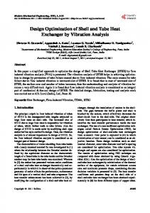
2. Reliability Assessment Approach [Al-Habahbeh, 2011] The Reliability Prediction flow chart is shown in Fig. 1. It consists of two loops connected by the Probability Density Functions (PDF) of heat transfer coefficients. The left hand side loop represents the stochastic CFD simulation stage, and the right hand side loop represents the stochastic FEM stage.

480

Physics-Based Reliability Assessment of a Heat Exchanger Shell

Fig. 1: Reliability Assessment Method

3. Reliability Assessment of the Heat Exchanger Shell As a critical part of the heat exchanger, the occurrence of failure in this component leads to leaking and eventual failure of the whole heat exchanger. Therefore, the above Reliability Prediction approach is applied to this component. The location of the component within the system is shown in Fig. 2. The system comprises four components; Heat exchanger, moisture separator, and two expansion joints (supply and return). The heat exchanger circuit is installed between the Low Pressure Compressor and the High Pressure Compressor of the gas turbine. The heat exchanger increases the turbine efficiency by cooling air before it enters the High Pressure Compressor [Gas Turbine data, 2007]. Therefore, the reliability of these components is critical to the operation of the gas turbine.

Supply Expansion Joint

Gas Turbine

Return Expansion Joint

Heat Exchanger (consists of shell and tubes bundle)

Moisture Separator

Fig. 2: Gas Turbine Cooling System [Gas Turbine data, 2007]

The application of the Reliability Prediction method to the heat exchanger circuit is a complex task. Here, the focus will be on the heat exchanger shell. The employed reliability method depends on the 481

O.M. Al-Habahbeh, D.K. Aidum, P. Marzocca

Physics-based Modeling which consists of two phases; CFD and porous media for the fluid side and FEM/Fatigue for the structure side. Physics-based modeling is used in conjunction with reliability methods. The main interest in this work is to analyze the transient start-up of the component, and to achieve this goal, the system is modeled using transient analysis. As a result of heat flux, temperature gradients develop and induce thermal stresses in the structure. The calculated heat transfer coefficient is for air convection, while the mode of heat transfer within the structure is conduction. The Reliability assessment method is performed by integrating several software packages that include iSIGHT®, ANSYS/DesignXplorer®, CFX®, and Simulation®. The reliability of the component is based on thermal stress fatigue as the failure criterion.

3.1 CFD and Porous Media Simulation of the Heat Exchanger Air Side In order to simulate the air effect on the heat exchanger shell, a CFD simulation of the inner air should be conducted. The shell houses the water tubes bundle as well, however, we are only interested in the air part which affects the inner surface of the shell. Due to its complexity, the heat exchanger bundle is modeled using porous media approach. In the course of the FEM thermal analysis which is part of the reliability analysis, thermal cyclic stresses are considered more important than mechanical stresses [Metals Handbook, 1987], this effect is taken into consideration in this work as will be discussed later. As the bundle is too complex to be modeled using direct simulation methods, an alternative approach is used to reduce the complexity of the bundle. This modeling approach is based on saturated porous media concept. The technique consists of treating the bundle as a fluid saturated porous medium, and using the volumeaveraged velocity, the pore Reynolds number, and a dimensionless pressure gradient group. Another reason for pursuing this direction is that the heat and fluid flow process can be simulated numerically if the heat exchanger is replaced at every point by a porous medium with volume-averaged properties [Nield, 2006].

3.2. Porous Media Approach [ANSYS® manual, 2008] The porous model is at once both a generalization of the Navier-Stokes equations and of Darcy's law commonly used for flows in porous regions. It can be used to model flows where the geometry is too complex to resolve with a grid. The model retains both advection and diffusion terms and can therefore be used for flows in rod or tube bundles where such effects are important.

In

deriving

the

continuum

equations, it is assumed that ‘infinitesimal' control volumes and surfaces are large relative to the interstitial spacing of the porous medium, though small relative to the scales that need to be resolved. Thus, given control cells and control surfaces are assumed to contain both solid and fluid regions. 482

Physics-Based Reliability Assessment of a Heat Exchanger Shell

The volume porosity ` at a point is the ratio of the volume V  available to flow in an infinitesimal control cell surrounding the point, and the physical volume V of the cell. Hence: V   ` V

(1)

It is assumed that the vector area available to flow, A , through an infinitesimal planar control surface of vector area A is given by:

A  K  A

(2)

  is a symmetric second rank tensor, called the “area porosity tensor”. The dot product of

where K  K ij

a symmetric rank two tensor with a vector is the vector: K  A  K Aj . The general scalar advectioni

ij

diffusion equation in a porous medium becomes:

  `       K U       K    ` S t

(3)

where, t is time, ` is volume porosity, ρ is density (kg/m3), K is area porosity tensor, U is true velocity (m/s), and S is source term. In addition to the usual production and dissipation terms, the source term S will contain transfer terms from the fluid to the solid parts of the porous medium. In particular, the equations for conservation of mass and momentum are:

 `      K U   0 t

(4)

and:





 T  `U        K U   U     e K  U   U  t

  ` R U  ` p

(5)

where U is the true velocity,  e is the effective viscosity (either the laminar viscosity or a turbulent

 

quantity), and R  Rij

represents a resistance to flow in the porous medium. This is in general a

symmetric positive definite second rank tensor, in order to account for possible anisotropies in the resistance. In the limit of large resistance, a large adverse pressure gradient must be set up to balance the resistance. In that limit, the two terms on the r.h.s. of Equation 5 are both large and of opposite sign, and the convective and diffusive terms on the l.h.s. are negligible. Hence, Equation 5 reduces to: U   R 1   p

(6)

Hence, in the limit of large resistance, an anisotropic version of Darcy's law is obtained, with permeability proportional to the inverse of the resistance tensor. However, unlike Darcy's law, we are working with the actual fluid velocity components U , which are discontinuous at discontinuity in 483

O.M. Al-Habahbeh, D.K. Aidum, P. Marzocca

porosity, rather than the continuous averaged superficial velocity, Q  K .U .

Heat transfer can be

modeled with an equation of similar form:

  ` H       K UH      e K H   ` S H t where

e

is an effective thermal diffusivity and S

H

(7)

contains a heat source or sink to or from the porous

medium. An important parameter in porous media concept is the directional momentum loss model. It can be derived from the following general momentum equation for a fluid domain:    Ui    U jUi  p     gi  ji  SiM t x j xi x j

(8)

The momentum source, SiM can be represented by:

SiM  CR1Ui  CR2 U Ui  Sispec

(9)

where C R 1 and C R 2 are linear and quadratic resistance coefficients, respectively. S is p e c contains other momentum sources (which may be directional), and U is superficial velocity. A generalized form of Darcy's law is given by:

 where

 is the dynamic viscosity,

K

p    Ui  Kloss U Ui xi K perm 2

(10)

is the permeability, and K loss is the empirical loss coefficient.

p erm

The porous media concept is implemented in ANSYS/CFX® by comparing Equation 9 with Equation 10

to set the following coefficients:

C R1 

 K perm

C R 2  K loss

,

 2

(11)

Data may sometimes be expressed in terms of the true velocity, whereas ANSYS/CFX® uses superficial velocity. If so, the coefficients are represented by:

C R1 

  K perm

,

C R2 

K loss  2 2

(12)

where ` is the porosity.

3.3. Heat Exchanger Air Porous Model Porous media concepts have been widely used to model large and complex thermal equipment. In this work, due to its large size and high complexity, the heat exchanger bundle is modeled by porous 484

Physics-Based Reliability Assessment of a Heat Exchanger Shell

®

media approach [ANSYS

manual, 2008]. On the other hand, a full model is used for the shell

structure. The porous model contains fluid domains as well as porous domains. The air side is modeled independently from the water side [ANSYS, 2008]. The air side contains air domains in addition to porous domains for the bundle. Directional momentum loss is entered in the porous model to simulate pressure drop. Sub-domains are added to the porous models to simulate volumetric heat sinks, which represent water. The results of the porous model will be used as input to the shell model. The dimensions used in the porous model include width, height, and length of bundle, number of rows, shell length and diameter. The fins layout in the air pass of the bundle is important for the porous model setup. There are three stages where the fins come closer together as the air flow proceeds through the bundle. That is to limit the maximum temperature in the fins that face the hottest air. Bundle air porosity and permeability must be calculated. The geometric details of all fin stages are used to calculate the porosity. These details include total volume, fins volume, tubes volume, number of tubes/fins intersections, tube/fin intersection volume, total solid volume, and total air volume. On the other hand, the details of the flow areas of all fin stages are used to calculate the permeability. These details include flow projected area of fins, flow projected area of tubes, flow projected area of fins/tubes intersections, solid flow projected area, total flow projected area, and air flow projected area. In order to account for thermal effects in the porous model, it is necessary to insert appropriate heat sink. The heat sink will be inserted into the air porous model. The characteristics of water in all stages of the bundle are used to calculate the heat sink. These characteristics include water volume, density, mass, specific heat capacity, enthalpy, and energy. In order to estimate the amount of exchanged heat that is needed to address the thermal effects in the air porous model; water and air residence times in each stage of the bundle must be obtained. Residence times are calculated using the geometries and the flow velocities. The bundle inlet air characteristics are also needed for the simulation of the porous model. They include air temperature, pressure, and density. Since the modeling of uncertainty requires the application of Monte Carlo Simulation to the developed porous model, the porous model must be fully parametric. For example, the model will be used to simulate the velocity and temperature distributions according to inlet velocity and temperature. The stochastic CFD analysis of the air porous model is performed using ANSYS/CFX® and ANSYS/ DesignXplorer®. The Air porous model along with its boundary conditions is shown in Fig. 3. It consists of 3 air porous stages, inlet, and outlet. The third air porous stage (Stage III) is further divided into two sections (A & B) because it spans across the center of the bundle over the two water passes. These domains are listed in Table 1. Some domains are fluid and others are porous media. For each porous domain, a directional momentum loss is defined in the x-direction. This loss depends on the area available 485

O.M. Al-Habahbeh, D.K. Aidum, P. Marzocca

to flow (permeability) and the volume available to flow (porosity). In order to account for the thermal effects, heat sinks are inserted into the air porous domains. Heat sinks are calculated based on the amount of water corresponding to each air domain. Using the Enthalpy of water, water energy is obtained for each domain. This energy is divided by available time to find the rate of heat transfer. The available time corresponds to the water residence time, which is obtained by dividing the length of each water pass by the water velocity. By obtaining the above quantities, the model is ready for simulation. In the next step, the model must be tuned to reflect the behavior of the real system. For this purpose, a set of operational data is utilized. The data provides values of input flow rate, pressure, and temperature, in addition to output pressure and temperature. Two temperature points are used to tune the heat sinks, one is input temperature, and the other is output temperature. On the other hand, in order to tune the friction factor for momentum loss, the input and output pressures are used. The CFD mesh used is shown in Fig. 4.

Table 1: Domains of Air Porous Model Domain

Type

Details

Air in Stage I

Fluid domain Air porous media

Real air Contains heat sink I

Stage II

Air porous media

Contains heat sink II

Stage IIIA

Air porous media

Contains heat sink IIIA

Stage IIIB

Air porous media

Contains Heat sink IIIB

Fluid domain

Real air

Fluid domain (real air)

Real air

Air between stage 3B and moisture separator Air-out

486

Physics-Based Reliability Assessment of a Heat Exchanger Shell Air-in

Bundle Stage IIIA

Bundle Stage IIIB

Separating wall

Bundle Stage II Bundle Stage I

Air out

Wall (No slip/Adiabatic)

Fig. 3: Air Porous Model

Fig. 4: CFD Mesh of Air Porous Model (545,591 elements)

It is worth noting that this analysis does not aim to resolve the thermal boundary layers, but rather focuses on the conjugate heat transfer between the solid and fluid domains. Input parameters to the air porous model are shown in Table 2. However, selected input parameters that are marked with asterisks will become random variables as part of the stochastic CFD analysis of the Air porous model. The random distributions data for these selected parameters include statistical characteristics of Weibull 487

O.M. Al-Habahbeh, D.K. Aidum, P. Marzocca

distribution such as Shape Parameter, Characteristic Life, and Lower limit of the random variable

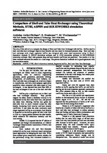
[ANSYS® manual, 2008]. After conducting the stochastic CFD analysis for the Air porous model, the main results of interest are temperature distribution, velocity distribution, and heat transfer coefficient. Fig. 5 shows the Temperature Distribution of the air in the porous model. It is clear how the air temperature reduces while passing through the bundle. Fig. 6 shows the heat transfer coefficient distribution in the air porous model. This information is important as it will be used to model the heat transfer at the inner wall of the Heat Exchanger shell.

Fig. 5: Temperature Distribution of Air Porous Model

In Fig. 6 there is a jump in the heat transfer coefficient along the wall dividing the two halves of the Heat Exchanger (the inlet air region which is the hotter half and the outlet air region which is on the right side). This can be explained by realizing that the heat transfer coefficient depends mainly on the velocity of the air flow, and therefore it is highest near the air inlet at the back of the left side. In addition, air is only allowed to pass through the bundle, and the areas above and below the bundle are separated by a wall as shown in Fig. 3.

488

Physics-Based Reliability Assessment of a Heat Exchanger Shell

Table 2: Input Parameters of Air Porous Model Parameter

Unit

Height of bundle

m

Inner diameter of Heat Exchanger

m

Length of bundle

m

Inner diameter of air outlet

m

Stage 1 and II volume porosity

Dimensionless

Stage 1 and II air permeability

m2 kg m2/s3

Heat sink stage 1 and 2 Stage 3A volume porosity

Dimensionless

Stage 3A air permeability

m2 kg m2/s3

Stage 3A heat sink Stage 3B volume porosity

Dimensionless m2

Stage 3B Permeability

kg m2/s3

Stage 3B heat sink Trap volume porosity

Dimensionless

Trap permeability

m2

Inlet air temperature

°C

Outlet static pressure

kPa

Air inlet mass flow rate

kg/s

Fig. 6: Heat Transfer Coefficient Distribution of Air Porous Model

The output parameters of the air porous model are listed in Table 3. Their statistical distributions characteristics are used for further CFD simulations. For example, the PDF of average heat transfer coefficient at the outer wall of the air porous model will be used for the FEM analysis of the shell model. 489

O.M. Al-Habahbeh, D.K. Aidum, P. Marzocca

The volume velocity in Table 3 refers to the velocity of air across the available space within the porous model. Table 3: Output Parameters of Air Porous Model Parameter

Explanation

Outlet T

Air average outlet temperature (°C)

Avg Vel

Average volume velocity in stage 1 and 2 (m/s)

AHTC1

Air Heat Transfer Coefficient left side

AHTC2

Air Heat Transfer Coefficient right side

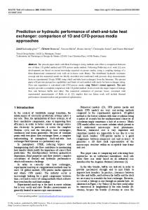
3.4. Heat Exchanger Shell The heat exchanger shell model is shown in Fig. 7. This model will be used only for the FEM analysis, because the CFD simulation of the shell involves the air inside the shell which was already simulated in the air porous model. Therefore, the results of that simulation are used here. Fig. 5 and Fig. 6 show the air model inside the Heat Exchanger shell. They depict the distributions of both temperature and wall heat transfer coefficient which are used for the shell FEM simulations.

Fig. 7: CAD Model of the Heat Exchanger Shell

The selected random input parameters for this model are marked with asterisks in Table 4. Their statistical distributions characteristics must be defined to perform the stochastic FEM simulations. After performing the stochastic CFD simulation in the air porous model, the CFD output parameters shown in Table 3 are obtained, along with their statistical distributions. These parameters are used for the shell FEM simulation. Meanwhile, all parameters used for the FEM analyses of the Heat Exchanger shell are shown in Table 4. A section of the mesh used for the FEM analysis is shown in Fig. 8. 490

Physics-Based Reliability Assessment of a Heat Exchanger Shell

Table 4: Parameters of Heat Exchanger Shell Parameter Compressive Yield Strength Convection Ambient Temperature

Unit MPa °C

Convection Film Coefficient

W/m2 °C

Water Pipe Outer Diameter

m kg/m3

Density Air Outlet Outer Diameter

m

Poisson's Ratio

---

Air Pressure

kPa

Thickness

m

Specific Heat

J/kg °C

Tensile Ultimate Strength

MPa

Tensile Yield Strength

MPa

Thermal Conductivity

W/m °C

Thermal Expansion

1/°C

Young's Modulus

Pa

Thickness

m

Maximum Shear Stress (Output) Fatigue Life (Output)

MPa Cycles

Fig. 8: Shell Finite Element Mesh

The CFD-computed temperature and heat transfer coefficients are imposed on the corresponding FEM model. A thermal transient analysis is conducted and the transient temperature distribution is shown in Fig. 9. It is noted that due to the separating wall between the inlet and the outlet regions of the heat exchanger (shown in Fig. 3), there is a line that separates the different temperatures of the 491

O.M. Al-Habahbeh, D.K. Aidum, P. Marzocca

two regions, where the inlet region is hotter. Thermal stress is calculated by conducting a structural analysis using the transient temperature state as input. The thermal stress distribution is shown in Fig. 10. The maximum thermal stress is determined by calculating and plotting stress at regular time intervals. Fatigue life of the shell model is computed using the stress results along with fatigue data. Life PDF is used to obtain the reliability of the shell model. The reliability can be determined directly from this table for a given service life. On the other hand, predicted life can be determined for a given reliability level.

Fig. 9: Transient Temperature Distribution in the Shell Model

Fig. 10: Maximum Thermal Stress Distribution

492

Physics-Based Reliability Assessment of a Heat Exchanger Shell

3.5. Stress-Life Estimation The maximum transient stress result is used to determine the corresponding stress-life of the component. The S-N curve shown in Fig. 11 is used for this purpose. Latin Hypercube technique is used to generate 28 maximum stress points. These points represent the variation in operational and environmental conditions as shown in the CFD and FEM analyses sections. Approximation surface regression is used to generate 10,000 points based on the original 28 points. Those points are used to plot the Life Probability Density Function (PDF) shown in Fig. 12. This PDF is used to calculate the reliability of the component as shown in Fig. 13.

Fig. 13: Semi-Log S-N Curve of the Model Material [ASME Code, 1998]

493

O.M. Al-Habahbeh, D.K. Aidum, P. Marzocca

Fig. 14: Life PDF

Fig. 15: Reliability Calculation using Life PDF

4. Conclusions The presented reliability assessment method can easily be used to predict the reliability of heat exchanger shell by means of stochastic physics-based modeling. By implementing stochastic CFD and FEM analyses, along with a stochastic porous model for the fluid effect, uncertainties of operational and environmental conditions such as flow velocity and temperature can be reflected into the reliability prediction process. Transient thermal analysis produces variable thermal stress. Therefore, critical stress can only be determined by investigating the whole transient phase. This integrated reliability assessment method is

494

Physics-Based Reliability Assessment of a Heat Exchanger Shell

a powerful method for designing heat exchanger shells with optimum performance and reliability. The porous media concept is a powerful technique for simulating and investigating flow characteristics in complex fluid-structure geometries. Since they approximate the actual system, Stochastic Porous Media (SPM) models can estimate uncertainties in flow conditions, which are used for subsequent CFD simulations of sub-models. Due to the complexity of CFD and FEM computations, performing stochastic simulations using direct MCS is computationally prohibitive. Instead, Latin Hypercube Sampling, Full Factorial Design, and Response Surface Models should be used. It is found that fatigue analysis parameters have a great effect on the result of the reliability assessment methods.

Acknowledgment The Authors would like to thank GE Energy, Texas, for their support of this research.

References Ahlinder, S., (2006) On Modelling of Compact Tube Bundle Heat Exchangers as Porous Media for Recuperated Gas Turbine Engine Applications, M. Sc. Thesis, Tag der mündlichen Prüfung. Al-Habahbeh, O.M., Aidun, D.K., Marzocca, P., and Lee, H., (2011) Integrated Physics-Based Approach for the Reliability Prediction of Thermal Systems, International Journal of Reliability and Safety, Vol. 5, No. 2, pp. 110-139. ANSYS® Reference manuals, (2008). Asghari, T. A., (2002) Transient thermal analysis takes one-tenth the time, Motorola Inc, EDN. Basaran, C., and Chandaroy, R., (2000) Using Finite Element Analysis for Simulation of Reliability Tests on Solder Joints in Microelectronic Packaging, J. Computers and Structures, V. 74, pp 215-231. Bedford, F., Hu, X., and Schmidt, U., (2004) In-cylinder combustion modeling and validation using Fluent. Boyce, R., Dowell, D. H., Hodgson, J., Schmerge, J. F., and Yu, N., (2004) Design Considerations for the LCLS RF Gun”, Stanford Linear Accelerator Center, LCLS TN 04-4, pp 21, Retrieved from: http://wwwssrl.slac.stanford.edu/lcls/ technotes/lcls-tn-04-4.pdf. Constantinescu, A., Charkaluk, E., Lederer, G., and Verger, L., (2004) A computational approach to thermomechanical fatigue, International Journal of Fatigue V. 26 pp 805–818. Fernández, E. U., Peterson, P., and Greif, R., (2007) Intermediate Heat Exchanger Dynamic Thermal Response Model, Doctoral Research, Advanced High Temp. Reactor (AHTR), U. C. Berkeley. 495

O.M. Al-Habahbeh, D.K. Aidum, P. Marzocca

Gue´de´, Z., Sudret, B., and Lemaire, M., (2007) Life-time reliability based assessment of structures submitted to thermal fatigue, International Journal of Fatigue. Gas turbine data, (2007). Hancq, D. A., (2004) Fatigue Analysis Using ANSYS, CAE Associates, http://caeai.com, pp 9. Ichiro, F., Naoto, K. A., and Hiroshi, S., (2006) Development of Thermal Transient Stress Charts for Screening Evaluation of Thermal Loads, Retrieved from: http://sciencelinks.jp/j-east/article/200613/000020061306A0496523.php. Jaske, C. E., (2000) Fatigue-Strength-Reduction Factors for Welds in Pressure Vessels and Piping, CC Technologies Laboratories, Inc., Dublin, OH. Lee, S. and Kim, I., (2007) Fatigue and Fracture Assessment for Reliability of Electronics Packaging, Korea Advanced Institute of Science & Technology. LeMasters, J., (2004) Thermal Stress Analysis of LCA-Based Solid Oxide Fuel Cells, Master’s Thesis, Georgia Institute of Technology, pp 25, 104. Liu, F., Ai, S. H., Wang, Y. C., Zhang, H., and Wang, Z. G., (2002) Thermal-mechanical fatigue behavior of a cast K417 nickel-based superalloy, International Journal of Fatigue, V. 24, pp 841–846. Metals Handbook, (1987) Volume 10, Eighth Edition, Failure Analysis and Prevention, American Society for Metals, pp 545-558. Nakayama, A., Kuwahara, F., and Hayashi, T., (2004) Numerical modeling for three-dimensional heat and fluid flow through a bank of cylinders in yaw, J. Fluid Mech, vol. 498, pp 139–159. Nield, D. A. and Bejan, A., (2006) Convection in Porous Media, 2nd ed. Springer. pp 87. Oberg, E., McCauley, C.J., (2004) Machinery's Handbook: A Reference Book for the Mechanical Engineer, Industrial Press Inc., ISBN 0831127376, pp 207. Personal Communications, ANSYS, 2008. Prithiviraj, M. and Andrews, M. J., (1998) Three Dimensional Numerical Simulation of Shell-And-Tube Heat Exchangers. Part I: Foundation and Fluid Mechanics, J. Numerical Heat Transfer, Part A: Applications, Vol. 33, Issue 8, pp.799- 816. Qylafku, G., Azari, Z., Kadi, N., Gjonaj, M., and Pluvinage, G., (1999) Application of a new model proposal for fatigue life prediction on notches and key-seats, International Journal of Fatigue 21, pp.753– 760. Rao, K. R., Editor, (2002) Companion Guide to the ASME boiler & Pressure Vessel Code, Volume 2, pp.139.

496

Physics-Based Reliability Assessment of a Heat Exchanger Shell

Satyamurthy, K., Singh, J. P., Hasselman, D. P. H., and Kamat, M. P., (1980) Transient Thermal Stresses in Cylinders with a Square Cross Section Under Conditions of Convective Heat Transfer, Journal of the American Ceramic Society 63 (11-12) , 694–698. Structural steel fatigue data at zero mean stress, (1998) ASME BPV Code, Section 8, Div 2, Table 5110.1. Theodossiou, V. M., Sousa, A. C. M., and Carlucci, L. N., (1988) Flow field predictions in a model heat exchanger, Computational Mechanics, Volume 3, Issue 6, pp 419-428. Vafai, K., (2000) Handbook of Porous Media, 2nd ed., Taylor & Francis, pp 236. Vandevelde, B., Gonzalez, M., Limaye, P., Ratchev, P., and Beyne, E., (2004) Thermal cycling reliability of SnAgCu and SnPb solder joints: a comparison for several IC-packages, IMEC, Kapeldreef 75, B-3001 Leuven, Belgium. Yang, G., (2007). Life Cycle Reliability Engineering, John Wiley & Sons, Inc. pp 1, 232.

497