Ford4, (6.10) gives 5η
Communications in Commun. math. Phys. 51,1—13 (1976)
Mathematical
Physics © by Springer-Verlag 1976
Particles and Scaling for Lattice Fields and Ising Models James Glimm* Rockefeller University, New York, N. Y. 10021, USA
Arthur Jaffe** Harvard University, Cambridge, Mass. 02138, USA
Abstract. The conjectured inequality Γ ( 6 ) ^0 leads to the existence of φ 4 fields and the scaling (continuum) limit for d-dimensional Ising models. Assuming Γ ( 6 ) ^0 and Lorentz covariance of this construction, we show that for d^6 these φ\ fields are free fields unless the field strength renormalization Z " 1 diverges. Let λ be the bare charge and ε the lattice spacing. Under the same assumptions (Γ ( 6 ) ^0, Lorentz co variance and d^6) we show that if λε4~d is bounded as ε->0, then Z " 1 is bounded and the limit field is free.
1. Introduction
Even φ 4 fields in the single phase region describe particles which interact through repulsive forces. The evidence in support of this statement includes the absence of even bound states [24, 3,34] the canonical lower bound on critical exponents [16], the arguments of [19] concerning absence of three-particle bound states and CDD zeros (which depend on the conjectured inequality Γ ( 6 ) ^0) and the (6) scaling and numerical arguments of [22,29] in favor of this Γ inequality for d ^ 3. 4 The purpose of this note is to extend some of these ideas to lattice φ field theories and Ising models. There are two reasons for studying lattice (as opposed to continuum) field theories. The first reason is that all dimensions, including d^4, are possible, and that the results obtained may be related to the existence [17,16,1,30,21] and triviality/nontriviality problems in these dimensions, see also [32, 33]. The second reason is that the lattice φ 4 field theory is an intermediate link between the continuum φ 4 field theory and the Ising model, and may serve to clarify the relation between Ising model and field theory critical behavior, see [20-22,26-27, 31]. Beyond these two reasons, we note that lattice field theories are at the outset easier because of the absence of ultraviolet problems but ultimately more difficult because of the absence of the Euclidean rotation symmetry. * **
Supported in part by the National Science Foundation under Grant MPS 74-13252 Supported in part by the National Science Foundation under Grant MPS 75-21212
J. Glimm and A. Jaffe Renormαlizαtion Scaling (continuum) limit group fixed point % of Ising models
Ising models
Ά Continuum field theories'
Lattice field theory
Region of canonical limit for d > 6 , according to ' Theorem 5.1 λ=O Trivial (Gaussian) renormalization group fixed point
Continuum limit of free lattice fields
y Gaussian (free) lattice fields
Fig. 1. The λφA+σφ2 parameter plane. ε= lattice spacing; σ=σ(λ, ε, m) chosen to give mass m in single phase region; m held fixed (e.g. m=l). The λ axis represents (continuum) field theory. The ε axis at A=oo represents Ising models [30]. The e axis at λ=0 represents Gaussian lattice fields. The curve λ=sd~4' represents constant dimensionless bare charge. Charge renormalization for d^4 may lead to a reparametrization of the λ axis
As a compensation for the loss of Euclidean invariance and of the resulting Lehmann spectral formula, we use the momentum space canonical upper bound [9] on the two point function, as well as the Γ ( 6 ) ^0 inequality as used in [19]. Our first main result assumes only Γ ( 6 ) ^0. The conclusion is the existence of a continuum φ\ field theory with an arbitrary choice of charge renormalization. Included is the existence of the scaling (continuum) limit for Ising models. The second main result assumes in addition Lorentz invariance of the continuum d 4 theory, as well as the (finite) charge renormalization, λ:gε ~ ,ε being the lattice d 4 spacing. Note that ε ~ ->0 in the continuum limit ε-»0, for d^5. In this case, the ε=0 theory is canonical for d^6 (§ 5). The limits considered here are summarized in Figure 1 above. Coincidence of the two fixed points seems to correspond to the picture in which nontrivial 4 φ field theories cannot be constructed as a limit of lattice cutoff approximations. Similarly, it would seem that the Ising model would be governed by the trivial fixed point only in the case for which a nontrivial fixed point does not occur in Figure 1. A renormalizability curve λ=O(εd~4) of constant dimensionless bare charge is indicated on this figure. A limit constructed along any such curve is renormalizable. Those limits constructed below this family of curves are superrenormalizable (e.g. the continuum limit with constant λ, d = l,2,3). Theories constructed above these curves are nonrenormalizable (i.e. λzAr~d-+co as ε->0). The charge 4 4 0 λ has dimension (length)**" , so that λs " is a dimensionless bare charge.
Particles and Scaling
3
2. The Wave Function Renormalization and Proper Self Energy for Noncritical Lattice Theories In this chapter, we consider a P(φ) lattice field or Ising model. We suppose that the infinite volume limit is defined and is invariant under lattice translations, rotations and reflections. We also assume FKG inequalities [6], a positive mass m > 0 (i.e. an exponential decay rate for correlations in lattice directions) and a single phase. These restrictions should be viewed as restrictions on the boundary conditions and/or coupling constants. In particular they are satisfied for φ* interactions and the Ising model approaching the critical point from a single phase direction. Let G(x)= -
^0
(2.1)
be the truncated two point function. The Fourier transform (2.2) (2
is nonnegative because G \x) is positive definite. Using invariance of G(2\x) under reflections and rotations, G (2h (p) is a symmetric function of the variable {cospv}^= 1 . Using the selfadjoint transfer matrix, one shows that .0,x v ,...0)
(2.3)
(2)
for any v [30]. In particular G has an exponential decay rate in all directions and G ( 2 h is analytic for p in a tube τ. By Hartog's theorem, τ is convex and also using the pv-^—pv symmetry, we see that p: £ | I m p v | ^ m l c τ c { p : s u p | I m p v | ^ m l . v=l
J
I
v
(2.4)
J
The use of Hartog's theorem can be avoided by a Schwarz inequality. For
Thus not only is τ convex, but its border coincides with the singularities of G{2)r{p\ for Rep=0. We have proved the following: Proposition 2.1. For a lattice field or Ising model as above, G{2)ris analytic in a convex tube τ, satisfying (2.4). We distinguish a single lattice direction x, and write x={x2,...,xd},p = {P2>'-> Pa)- The existence of a self adjoint transfer matrix means that G ( 2 h h a s an analytic continuation for px in the half plane p\ Φ neg. real, for p real. Proposition 2.2. Consider a lattice field or Ising model as above with p real Then G (2h (p) is Herglotz as a function of the variable 1 — cosp^ For some positive measure dρ(a, p) depending on p, d β i a P
\
, α
(2.5)
4
J. Glimm and A. Jaffe
and 0~(p)=-α0>)(l-cos P l )
f
--
1
a
dv{a,p)
(2.9)
with a ^ 0, β real, dv positive and
Remark. For d}±3, there is a constant K depending only on d and G(2>(0) such that (2.10)
\ Proof. By [9], t. | p Γ 2 .
(2.11)
Particles and Scaling
5
By the Herglotz property, used successively in each coordinate, as in the proof of Proposition 2.2, 2
(2
|p v Γ G >~(π,...,π). v=l
Thus for any r > 0 and for d > 3, (2)
d
(2)
G (0) = (2π)- ίG ~(p)dp ^ const./
j
|pΓ 2 dp + r- 2 d G ( 2 ) ~(π,...,π) N
l Here the optimal choice of r is
and so G
(2)(0)2d +1 ^
c o n s t
G
( 2 h ( π ? . . . ? π ) ^ const. G (2) ~(p).
A uniform upper bound on (2.9) follows. For d = 3, the exponents must be changed slightly to dominate rlnr in place of r, but a bound on (2.9) in still valid. Linear combinations of c o s p 1 = 0 , —1 show that β and oc + ^(a2 + l)~ίdv(a) are each bounded. Since α and dv are each nonnegative, the individual terms α and \{a2 + 1)~xdv are also bounded, proving (2.10). We now write x = (x\ x"\ p = (p\ p") for some decomposition x
=
(xί
9
? Xj) •>
x
— \xj+
1?
x
9 d)
of the coordinates, and consider the partial Fourier transform
Γ ( 2 V , p")= Σ e-ip"x"Γ(2\x\
x").
Proposition 2.4. Consider a lattice field or Ising model as above. For q + 0 , x2 =... = Xj = 0, p" real, Γ(2)~(x', p") is positive and has an exponential decay rate m^m. (Notej+0, by assumption.) Proof. First we consider the case x' = x x and p" = p. The Herglotz representation (2.9) in xί-space has three terms. The first is nonnegative for x ^ O . The second, proportional to β, vanishes for x t Φθ. The third is positive for all x l 9 so the proof is complete in this case. The general case follows from the case just considered, because integration with respect to p 2 , . . . , p 7 is equivalent to evaluation at x 2 = ... = X;=0. Definition. If the measure dρ(a,p = 0) has a ^-function at a= — 1+coshm, then Z > 0 is the strength of this (5-function. Otherwise by definition Z = 0. Proposition 2.5. For a pure phase lattice P(φ) field theory or Ising model with m>0andZ>0,
= α(0)+ J(α-coshm+lΓ 2 dv(α,0) o
(2.12)
6
J. Glimm and A. Jaffe
Proof. We write 1— cospi + α — 1 + coshm + ε
where
J
dρ-^0 as e-»0. Thus as cosp^coshm,
- 1 + cosh m 1
and the derivative of Γ
(2)
(2.12a)
1
can be evaluated as Z " from this inequality.
Remark. We have not assumed an upper mass gap, in contrast to [19]. Definition. C L m o is the free (Gaussian) lattice covariance, d
-1
- l + c o s h m 0 + 2] ( l - c o s P v )
(2.13a)
v=l
and Π~{p) = Γ{2y{p) + CZX0
(2.13b)
Proposition 2.6. Consider a lattice field theory with the hypotheses of § 2. Let P o , Px be projections onto the vacuum Ω( = 1) and the span of(\ — P0)φΩ respectively. Then Π(x) = - {x> = 0, x")(\ -Po-
PJP'φ)}
is positive definite and hence the Fourier transform of a positive measure.
3. Three Particle Decay for έP(φ)= φ4 In this section we consider λφ4 + σφ2 lattice field theories with σ>σc. Then all hypotheses of §2 are satisfied. Ising models are excluded because we integrate by parts.
Particles and Scaling
7 i6
Proposition 3.1. Assume Γ \xxxyyy) ^0 for x—y large. Then the CDD radius (6) m satisfies m^3m. The analyticity tube τΓfor Γ satisfies {p:Σ\Impv\^3m}CτΓ Proof. As in [19]. See also Proposition 3.2 below. This result leads to the existence of φ\ field theories and the scaling limit for Ising models, see §4. In order to establish the triviality of some of these field theories, we need to assume canonical upper bounds for the two point decay rate (as would follow from the Lehmann spectral formula in the continuum case). Explicitly, we assume
κ^x\
,|x|sm
e
This bound is always satisfied for fixed σ, λ, but eventually we will consider the postulate that Kx is independent of σ and/or λ, which is not known. Proposition 3.2. Assume (3.1) and Γi6)(xxxyyy)^0 theory with σ>σc. Then for
for a λφ* + σφ2 lattice field
where K2 is a universal constant and Kί is defined by (3.1), -3m\Xl\
for
..
(3.2)
Proof. As in [19], we expand Π in terms of connected and one particle irreducible subdiagrams. Negative terms, including Γ ( 6 ) can be omitted, yielding the bound Π(Xl, p = 0) ^ Σ x
χ l
(2)
3
(4)
(2)
(4)
J6G (x) - 36 Σ G (xx0z)Γ (z - z')G (zΌ0x)l. I
z,z'
(3.3)
J
By Lebowitz' inequality, G 4 ^ 0 . Let Pj be the momentum variable conjugate // =: to Zj—z'j. By Proposition 2.4, applied with p = (P2> ?Pd) 0> the terms with zί—z'ίή=0 may be omitted. Having done so, we apply Proposition 2.4 again with zί—z'1=0,p" = (p3,...,pd) = 0; we omit terms with z 2 Φz' 2 . Continuing in this fashion we have
where Proposition 2.7 provides the lower bound on Γ (2) (0). Lebowitz' inequality bounds the G ( 4 ) factors above, so that
+ ί44(2d-1 + 0 above is Euclidean invariant. Then it is a free scalar field of mass m. Proof The two point function is free by the theorem, and the theory as a whole is free by [35, p. 163]. Proof of Theorem 5.2. Let ΓJ m ε (p) be the inverse propagator for the theory with bare charge λ, mass m and lattice spacing ε. By scaling, Γsd-*λ,s-imJp)=s~2Γλ,m,s(sp).
(5.2)
Here we choose ε= 1, s->0, and 1
i.e.
m = const. s->0
so that the λ on the right side of (5.2) is bounded, but possibly s-dependent as s->0. Now Γλ m?ε(Pi,0) has a zero at cosp = coshm and as we have just seen, bounded first and second derivatives with respect to p1 evaluated at p = 0, pί = 0(m). Furthermore the first derivative vanishes at pί = 0 because of the pί-> — px symmetry. The same method bounds one more pί derivative, and
as s->0. This completes the proof. Remark. The vanishing of Γ on the mass shell gives a cancellation which formally allows d ^ 5 in place of d ^ 6 above. 6. Upper Bounds on Critical Exponents We give upper bounds on certain critical exponents in a single phase φ4 + σφ2 (lattice) quantum field model. In particular we study the anomalous dimension η, the exponent ζ for the field strength renormalization constant Z and the exponent v for the physical mass. We choose σ>σc (the single phase region) and consider the limit σ^σc. In this section we assume Γ ( 6 ) ^ 0 , as well as the x-space upper bound G
(2)
1
(d
2+
(x,σ)^K(min{M,m- })- - ^-
wW
(6.1)
with K uniform in the allowed x, σ. We expect (6.1) to hold for lattice field theories. We then show η = O = ζ for d ^ 5 , complementing the results of §5. Proposition 6.1. For a pure phase λφ4 + σφ2 (lattice) field theory with m>0, Z > 0 and satisfying (6.1), we have (6.2)
If in addition Γ ( 6 ) ^ 0 , then (6.3)
Particles and Scaling
11
Here ζ is the exponent for the field strength renormalization constant and v is the exponent for the mass. Thus Z~mζlv as m->0. Proof. Using (2.12a) evaluated at p1 = 0 gives m~2 Sconst. Z ^ G ^ O , * ) . We bound G2~(0, σ) by integrating (6.1) to obtain 2
1
η
2
m" ^const. Z~ m ~
.
Thus m~ηZ^const., or
Since the inequality O^η is known we have established (6.2). Assuming Γ ( 6 ) ^ 0 , we may use (5.1). Then -ζlv
m
We show ΣΠ(x)^ const., from which we infer proving ζ/v ^ 2. The summability of Π(x) follows from ΣΠ(x) = 2Γ(0) = 0(1) + Γ~(0).
(6.4) 1
Consider σ in the interval (σc9σ^ for σx>σc. Since Γ X 0 ) = - G ^ O ) " ^ , we need only bound F~(0) from below. However G2(x, σ) is decreasing in σ (a consequence of the second Griffiths inequality). Thus for σ>σc
is decreasing in σ and JH(O, σ) is also decreasing in σ. Thus Π(0, σc)Ξg/Ί(0, σ^. Theorem 6.2. Assume Γ η =
ζ/v==Q for
(6)
4
2
^ 0 and (6.1) m a λφ + σφ lattice theory. Then (6.5)
d^5
and for d^4
11.2 d=2
(6.6)
/! We use the bound (5.1) for m~ ζ / v ~Z~ 1 ^const. / l +
ΣxjΠixύ 3
^const. (ί+ΣxlίGix)
2
+ G{x) {G*G)(x)]j.
(6.7)
12
J. Glimm and A. Jaffe
Substituting (6.1) we find the G 3 term in (6.7) sums to (Km-*'2*-™),
(6.8)
2
while the G (G*G) term sums to
By Proposition 6.1, 2 —ί/^0 and (10-2d-4η)-(S-2d-3η)^0. Thus the G2(G*G) term in (6.7) dominates and by (6.2), (6.3), (6.7), (6.10)
proving (6.5). For d4, (6.10) gives 5η