Physics Sharpness of the Phase Transition in Percolation Models*

Communications in Commun. Math. Phys. 108, 489-526 (1987)

Mathematical

Physics

© Springer-Verlag 1987

Sharpness of the Phase Transition in Percolation Models* Michael Aizenman** and David J. Barsky Department of Mathematics, Rutgers University, New Brunswick, NJ 08903, USA

Abstract. The equality of two critical points - the percolation threshold pH and the point pτ where the cluster size distribution ceases to decay exponentially is proven for all translation invariant independent percolation models on homogeneous d-dimensional lattices (d^ 1). The analysis is based on a pair of new nonlinear partial differential inequalities for an order parameter M(β, h\ which for h = Q reduces to the percolation density P^ - at the bond density p = l—e~β in the single parameter case. These are: (1) M^hdM/dh + M2 + βMdM/dβ, and (2) dM/dβ^\J\MdM/dh. Inequality (1) is intriguing in that its derivation provides yet another hint of a "φ3 structure" in percolation models. Moreover, through the elimination of one of its derivatives, (1) yields a pair of ordinary differential inequalities which provide information on the critical exponents β and δ. One of these resembles an Ising model inequality of Frόhlich and Sokal and yields the mean field bound (5^2, and the other implies the result of Chayes and Chayes that β^ί. An inequality identical to (2) is known for Ising models, where it provides the basis for Newman's universal relation /?((5 —1)^1 and for certain extrapolation principles, which are now made applicable also to independent percolation. These results apply to both finite and long range models, with or without orientation, and extend to periodic and weakly inhomogeneous systems. 1. Introduction

There have traditionally been two different notions of a critical point in percolation models, corresponding to the boundaries of the low density and the high density regimes. For the standard one parameter percolation models on the ddimensional square lattice Έd (i.e. site percolation or nearest neighboor bond

* Research supported in part by the NSF Grant PHY-8605164 ** Also in the Physics Department

490

M. Aizenman and D. J. Barsky

percolation) the two critical densities are usually denoted by pτ (or πc) and, correspondingly, pH (or pc). The main result reported here is the proof of the equality of these two critical points. Expansion methods show that in the "high density" regime there is percolation (in two or more dimensional models, and in long range models in one dimension), while in the "low density" regime the cluster size distribution has exponential decay and the connectivity functions decay rapidly. Our main result is that these two phases extend up to a common critical point, without there being an intermediate phase in which with probability one there is no infinite cluster but the density of large cluster decays only by a power law. The coincidence of the two critical points is proven here for general translation invariant independent models - which may include long range and/or oriented bonds - in any dimension. Although such an assertion was expected by the physicists to be true - at least in the finite range case - previous mathematical treatments of the subject dealt successfully only with percolation models in dimensions d = 2 and d = \. The former case included, of course, the celebrated proof of Kesten [1] for self similar models, and its extension by Russo [2] to other finite range two dimensional models. The reference to d = 1 concerns, in addition to the trivial case of finite range models, also the rather special l/|x — y\2 models for which the coincidence of the critical points was derived in [3], by very different means. (Incidentally, the latter models exhibit also an intermediate phase, but within the high density regime [4].) It may also be of interest to compare our results for percolation with the results of Aizenman [5] on the analogous problem for ferromagnetic Ising spin models. For the Ising (and related) spin systems, the equality of the high and low critical temperatures was proven only under a certain "regularity" hypothesis, whose verification required certain restrictions. The arguments presented here require no such hypothesis, and suggest that although the regularity is indispensable for some of the other results derived in [5], it is not so for the 1 coincidence of the critical temperatures. Since translation invariance is the only assumption which is required here for independent systems, let us also remark that there are known examples of systems which are highly noninvariant for which pτ does not equal pHί Chayes and Chayes [6]. Before completing the summary of the results, and their relations with previous works, let us present the full definition of the two critical points pτ and pH, and introduce the notation we shall use for general independent percolation models. In the rest of the introduction we shall focus on (unoriented) bond percolation models, for which the length of the bonds need not be bounded. Oriented percolation, and partially oriented percolation (which we introduce in order to have a unified analysis), are discussed in Sect. 2.1. Site percolation and some other cases to which our analysis extends are discussed in Sects. 7 and 8.

1

This result has now been derived and is presented in a companion paper, coauthored with Fernandez [22]

Sharpness of Percolation Transitions

491

1.1. The Setup The basic example of a percolation transition is observed in the nearest neighbor bond percolation model on the cubic lattice JL = Zd. For this model, bonds are pairs of neighboring lattice sites. Each bond b = {x, j;} has associated to it a random variable nb which can take one of the two values : 0 or 1 . If nb = 1 , we refer to the bond b as "occupied." The variables {nb} are jointly independent and hence their distribution is completely characterized by the density of the occupied bonds : p = Prob(τι6 = l).

(1.1)

For a given configuration of the bond variables we regard the occupied bonds as connecting, and decompose the set of lattice sites into the corresponding connected components. We denote by C(x) the connected cluster of site x elL, and by |C(x)| its size i.e., the number of lattice sites in it. Some key quantities of interest are i) the expected size of the cluster containing a given site, say the origin 0: (1.2)

and ii) the probability that the origin belongs to an infinite cluster, i.e., the percolation density: M(p) = Prob(|C(0)| = oo).

(1.3)

The quantity M(p) is more often denoted by P^, which is consistent with the general notation for the cluster size distribution: Pn = Prob(|C(0)| = n).

(1.4)

Well known arguments show that for small enough p [in particular p < (2d — 1)" *] the expected cluster size χtotal(p) is finite. Furthermore, the finiteness of χioiΛι(p) is a good criterion for the low density phase. For example, it is known to imply exponential decay of the cluster size distribution [7, 8]. At the other extreme, for p close enough to 1, not only does χtotaι(p) diverge, but also there is a positive probability that the origin belongs to an infinite cluster (M(p) > 0). For such values of p the probability of generating an infinite cluster somewhere on the lattice 1L - is one. The two critical densities to which we referred above, are the boundaries of these high and low density regimes. Their natural definitions are pτ = nc = sup {p I χtotal(p) < oo } , and

(1.5)

Obviously, pτ^pH. In the more general class of independent bound percolation models, any two sites may be directly connected by an occupied bond; however, the probability of bonds to be occupied decreases for long bonds. Thus the set of bonds consists of all pairs of lattice sites, and with each such pair b = {x, y} we have associated an occupation random variable nb. The bonds are occupied independently with the

492

M. Aizenman and D. J. Barsky

translation invariant probabilities = ί) = Kb = l-e-βJ* *9

(1.6)

for b = {x,y}. The parameter β ( ^ 0), which is in a way redundant, is introduced both for mathematical convenience and because it allows the analogies with ferromagnetic spin models to be seen more clearly. It is most convenient to study the percolation transition by varying β at fixed values of the parameters Jxy (^0). The critical values βτ and βH are defined by the same criteria as pτ and pH in (1.5). It should be noted that the class of percolation models described by (1.6) includes long range models, for which Jx y decays slowly, e.g. Jx y = l/\x — y\s. While finite range models exhibit percolation only in dimensions d^2, such long range systems may percolate even in one dimension (iff s ^ 2 [9]). To avoid models with βH = 0, we assume that \J\=ΣJo,*«x> (1-7) X The results in this paper apply to all such systems. Other independent percolation models covered by our analysis include oriented percolation - for which one has only to reinterpret the notions used in our discussion of ordinary bond percolation (see Sect. 2.1) - and site percolation for which the adjustments are found in Sect. 7. Furthermore, one may replace the translation invariance requirement with periodicity or even weaker conditions (see Sect. 8.1). 1.2. The Main Results Our main results are the following two propositions. They apply to the percolation transition which is observed by varying one of the parameters of the model. The parameter is either p, as in (1.1), or β for the more general case derived by (1.6). For the former case no other parameter was introduced; however, in the more general case we also could have chosen to look at the transition produced by varying the bond densities of bonds {x,y} with given values of y — x. The results would be the same. Theorem 1.1. For any independent translation invariant bond, or site, percolation d model on Z (like the bond models introduced above), βr = βπ

or

> when applicable,

Pτ= Pπ-

(1-8)

We shall denote the common value in (1.8) by βc (or pc). To state the second result, which is in fact used in the proof of Theorem 1.1, let us define [extending 1-

Σ

1 5Ξ«< oo

Pn(β)e~nh.

(1-9)

The quantity M is of interest because it contains the Laplace transform of the cluster size distribution, because of its analogy with the spontaneous magnetization in ferromagnetic models, and because of its utility in the derivation of the above result.

Sharpness of Percolation Transitions

493

Theorem 1.2. Under the same assumptions as in Theorem 1.1 (independence and translation invaήance), M(βτ,h)^ const h1/2.

(1.10)

Let us remark here that, making sufficiently strong assumptions on the existence of power laws, it is customary to define the critical exponent δ by the relations or

P^H(βτ)=

Σ Pm = n-llδ.

m^n

(1.11)

For the sake of concreteness, we shall define δ by: 5 = l i m i n f — r^-ΓT . fc\o lnM(/J Γ ,Λ)

(1.12)

The result (1.10) shows that quite generally this exponent obeys the mean field bound: (1.13)

δ^29

which is in fact saturated (δ — 2) in the case of percolation models on a Bethe lattice. The proofs of these two theorems are based on a number of differential inequalities which are also of independent interest. In particular, we prove that for bond percolation models, in the generality described above, the quantity M satisfies:

and (1.15) (in the weak sense, as explained in Sect. 3). These inequalities are closely related to previous results of other works on percolation and ferromagnetic systems. We shall mention some of those below. Let us first however make some additional remarks on the nature of these inequalities. The differential inequality (1.14) is identical to one obeyed by the magnetization in ferromagnetic Ising spin systems, for which it follows from the GriffithsHurst-Sherman inequality [10]. Newman has pointed out that (1.14) bears an amusing relation to the Burgers equation, and furthermore, that it implies the critical exponent inequality [11]: (1.16)

β(δ-ί)^l

for models with βτ = βH. Here β is the critical exponent which enters in the expected power law: .

(1-17)

Newman's observation was extended in [12] to a number of useful extrapolation principles, which are now made applicable also to percolation (see Sect. 6). It is

494

M. Aizenman and D. J. Barsky

interesting to note that the inequality (1.16) is saturated in both percolation and ferromagnetic systems by the mean field (or Bethe lattice) values of the two critical exponents - despite the fact that individually these exponents take on different values in the two systems. The relation (1.15) is truly remarkable. A coarse glance at its derivation shows that hidden in it are some key features of percolation models which (like the previous work of [13] and the rigorous results of [8]) indicate a relation with a "φ3" field theory. Furthermore, combined with more general properties of the "order parameter" M [like (1.14)], the inequality (1.15) unifies previous results which dealt separately with the regimes: R1 = {β = βτ, h>Q} and R2 = {β>βH, h = Q}, and leads also to a proof of the equality βτ = βHOur derivation of the inequality (1.15) grew out of an attempt to understand the relation between the recent result of Chayes and Chayes [14], who proved (under a harmless assumption) ^—-,

(1.18)

and the inequality M

dh\h

3

+^,

(1.19)

which we had previously derived by means which are very different from the proof given below. Here inequality (1.18) is presented in its site percolation version and 1^1 = ΣK{o,X} Csee (1-6)]. In the original derivation of (1.19), which may equivaX

lently be stated as dM

M

y,

(2. la)

Prob(n (Xty) = l) = Prob((x,)0 is occupied)- ί-e~βjχ~*y,

(2.1b)

and

496

M. Aizenman and D. J. Barsky

where Jx>y, Jx^y, and Jy^x are regarded as separate parameters (and in general are not equal). However, we will assume that the couplings J are translation invariant, meaning that for all x, y, and z: an
y + z= Jχ^ y

(2-2)

A path from the site x to the site y is a sequence of bonds whose arrangement satisfies the obvious incidence relations. That is, the bond (u, v) may appear only in the step which proceeds from u to v and not vice versa, whereas {u, v} may be used in both directions. The cluster of x, C(x), is now defined (for a given bond configuration) to be the set of all sites y for which there exists a path of occupied bonds from x to y. (Note that the set of clusters of the sites of Tίά no longer offers a disjoint decomposition of the lattice.) With this definition of the cluster we continue to define the quantities Pn by (1.4). The expected cluster size χtotal and the order parameter M are still given by (1.2) and (1.9). Finally, we modify the symbol \J\ to mean:

M = Σ ( Ό., + ^x). X

(2-3)

Obviously, the unoriented models described in the introduction may be regarded as special partially oriented models, with Jx_+y = 0. However, it is also the case that a reader interested in only the more standard (unoriented) models may read the rest of the paper ignoring the fact that our notions were generalized in this subsection. 2.2. The Ghost Field Representation for M(β, h) We shall now introduce a construction which provides a useful probabilistic interpretation of the order parameter M(β, h) - extending the intuition one has forP^. For that purpose, we augment the model by adding to it random site variables {mx}xeZd (mx = Q, or 1). Probabilities are assigned so that {nb,mx} forms a jointly independent set of random variables, with Pτob(mx -1) -1 - eh (^ft,for ft small)

(2.4)

d

for every xeZ , and with Prob(rc& = l) still given by (1.6) or (2.1). For a given configuration {nb,mx} of bond and site variables, we denote by G the set of sites x with mx=ί and call these sites "green." (These are sometimes referred to as "ghost" sites, as in [17, 12].) We continue to define the connected cluster of x as above and we say that x is connected to the green set if at least one site in C(x) is green. Proposition 2.1. For the augmented system defined above, with h > 0, Prob(C(0)nG Φ0) = Prob(0 is connected to G) = M(β, h), where M is the order parameter defined in (1.9).

(2.5)

Sharpness of Percolation Transitions

497

Proof. First observe that for any nonrandom set Ac%d, ProbμnGΦ0) = l- Π e~* = l-έΓ* μ ι , xeA

(2.6)

where |^l| = card(^4). On the left-hand side of (2.5), condition on the cluster of the origin: Prob(C(0)nGΦ0) = Σ ProbμnGΦ0|A = C(0))Probμ = C(0)). ACZd

Note that the events ",4nGφ0" and "v4 = C(0)" are independent, as the first depends only on site variables and the second depends only on bond variables. With (2.6), we obtain Prob(C(0)nGΦ0) = £ Combining this relation with the fact [see (1.4)] that Σ

A:\A\=n

yields

Prob(^ = C(0)) = PB

« Prob(C(0)nGΦ0) = Σ Λ(l -e~nh) = l - Σ V* l^n^oo

n— 1

The n = oo term would make no contribution to the sum on the right-hand side (since h > 0) and for this reason is not included. Π Although (2.5) is valid only for positive values of ft, M(β, ft) is defined by (1.9) also for ft = 0 and, in fact, M(β, 0) = P^β). Since M is clearly continuous from the right at ft = 0, Proposition 2.1 shows also that limProb(C(0)nGΦ0) = P 0 0 .

Λ\0

This limit suggests that the green sites may be regarded as surrogates for the point at infinity. The green sites evacuate every finite region in Zd as ft vanishes. In this sense, the event "the origin is connected to the green set" is a small ft approximation to the event "the cluster of the origin is infinite." Because of certain analogies with Ising spin systems, we denote the order parameter by M, the symbol used for the magnetization in those models. The independent variable ft plays the role of an external magnetic field. As in the case of Ising models, we define the susceptibility to be the derivative of M with respect to ft: On

n

=ι

e"*9

ft>0.

(2.7a)

The definition of χ is extended to ft = 0 by continuity: χ(β, 0) = lim χ(β, h)= Σ nPn = , Λ\0

(2.7b)

ιι=l

where /[ — ] is the indicator function which vanishes when the cluster is infinite.

498

M. Aizenman and D. J. Barsky

For β 0, χ = .

(2.9)

Proof. Since the distribution of the green sites is independent of the bond variables, it is convenient to evaluate the right-hand side of (2.9) by first conditioning it on the bond configuration. The conditional expectation of the indicator function is exactly e~h\C(0^9 and hence

-^-χ. D Remarks. 1) As the above argument shows, for positive h there is no contribution in (2.9) from the event that the cluster of the origin is infinite. For an expression which is valid also at h = 0, one should modify the right-hand side of (2.9) by explicitly adding the restriction that |C(0)| < oo. 2) The following is a simple but convenient trick which is frequently of use. Since |C(0)|=Σ/[xeC(0)], X

we have by Proposition 2.2 that for Λ > 0 χ = Σ.

(2.10)

Observe that the summand in (2.10) converges in the h \ 0 limit to the probability that the origin is connected to x and the cluster of the origin is finite. This is one of the natural notions of the truncated two point connectivity function. 2.3. The Finite Volume Approximation Here we introduce the finite volume quantities and state their basic relation with the corresponding functions for the infinite lattice. The reasons for considering finite systems are: (i) all of the quantities of interest (in particular the order parameter) are trivially analytic in /?, (ii) the derivations of the main inequalities (1.14) and (1.15) rely on Russo's formula, the application of which is immediately valid only on a finite lattice, and (iii) the proof of (1.15) additionally uses the van den Berg-Kesten inequality which also has an initial finite lattice requirement. In order to maintain translation invariance at finite volume, we shall study percolation on the cubes ΛL = ( — L,L\dr\TLά with periodic boundary conditions. The periodic models are defined by setting the bond occupation probabilities, for

Sharpness of Percolation Transitions

499

with (2.12)

and similarly for the oriented bonds with the finite volume oriented couplings «4L_Ir Remark. There are also other natural boundary conditions which may be imposed on AL (e.g., the wired and free boundary conditions discussed in [1 8]) but they have the disadvantage of lacking homogeneity. We let P(n} = P(n\β) = ProbL(|C(0)| = n) ,

(2.1 3)

and define the finite volume order parameter and susceptibility by ML(β9h) = ί- Σ P(n\β}e~n\

(2.14)

w=l

and P/Lf

The finite volume order parameter and susceptibility have probabilistic interpretations similar to those of their full volume analogues. As in the preceding section, it is easily verified that ML = ProbL(C(0)nG Φ 0) .

(2.16)

That is, Proposition 2.1 holds at finite volume. Likewise, a finite volume positive h version of Proposition 2.2 can be proved by repeating the arguments of Sect. 2. 1 . In particular, we obtain the identity XL=

Σ ProbL(xeC(0), C(0)nG = 0).

(2.17)

xeΛL

Information about finite volume quantities is translated into information about full volume quantities by taking the "infinite volume limit." Proposition 2.3. For any /? ^ 0 and h > 0,

ML(β/0 — MOM),

(2.18)

and ) x C M )

(2.19)

Remark. For Λ = 0, (2.18) certainly fails if β>βH. If in addition χ(β,0)0be fixed. Then M and ML are increasing, concave and analytic functions of h, for h>0. We next consider the ^-dependence of M(β, h). When h = 0, we have M(β, 0) = P^(β\ and thus M(β,0) is clearly nondecreasing in β. In fact a stronger statement, which is a consequence of Proposition 2.1 and its finite volume version (2.16) is true. Lemma 2.5. At any fixed value of h (^0), M and ML are nondecreasing functions of β. The question of the analyticity of the order parameter is more difficult to resolve at the level of generality considered here. The following lemma summarizes some of what is known in this direction. For proofs, see the Appendix. (These results will not be used in this paper.) Lemma 2.6. (i) M is a continuous function of β for h>0 and all β^O and - in the unoriented case - also for h = 0 and β=¥βH. (ii) In finite range percolation models, M is an analytic function of β for h>0 and β>0.

3. Derivation of the Main Differential Inequalities In this section we consider the finite volume periodic models introduced in the preceding section and prove the differential inequalities upon which Theorems 1.1 and 1.2 rest. In subsequent sections we will integrate these inequalities at finite volume and then take the infinite volume limit. The two inequalities obtained and employed in this manner are found in the following propositions. Proposition 3.1. In a finite volume periodic model with ML and χL defined by (2.14) (2.15), (3.1)

Proposition 3.2. With the same hypotheses as above,

(3.2) Remarks, i) The quantity \J\ enters (3.1) as

£ (J(^x + J(o^x), which by our choice

X^ΛL

of finite volume couplings in (2.12) equals

£ (^o * + «Λ)->;c) = kl Csee (2.3)].

xeZd

ii) The above inequalities are finite volume versions of (1.14) and (1.15). In view of Proposition 2.3 the inequalities extend trivially to distributional inequalities for

Sharpness of Percolation Transitions

501

the infinite volume order parameter M(β, h\ for h > 0. ί Note that for this purpose, in (3.2) one should rewrite ML^—- as ^-^.} When M is differentiable (see op

2

op

J

Lemmas 2.4 and 2.6), those inequalities are valid in the classical sense. The above observation could be used for an alternative direct derivation of the infinite volume results reported here. We shall however use (3.1) and (3.2) in the more explicit way outlined at the beginning of this section. 3.1. Proof of Proposition 3.1 Before stating the differentiation formula which is used, let us introduce some technical terms. Definition. The event E is increasing with respect to the bond variables {nb} (or the site variables {mx}) on ΛL if the indicator function /[£] is nondecreasing in nb (respectively, mx) for every bond b (respectively, site x) in AL. An important example of an event which is increasing in both the bond and site variables is the event that the origin is connected to the green set: C(0)nGφ0. Definition. For a given configuration (nb, mx}, the bond b0 is called pivotal for the event EiiE occurs for {n(b\mx} but not for {n(b\mx}. Here {n^} (i= 1,0) are the bond configurations obtained from {nb} by requiring the bond b0 to be occupied (i = l) or unoccupied (z = 0). Note that the event that bQ is a pivotal bond is independent of the status of its occupation. With these definitions, we can now state a useful differentiation formula. Proposition 3.3 (Russo's formula [2]). // the event E is increasing with respect to the bond variables on ΛL, then for each bond b0, 3ProbL(£)

jbo

is piυotal far £)

ProbL(rcbo = 0, b0 is pivotal for E), where

Proof of Proposition 3.1. Recalling (2.16) and applying the Chain Rule followed by Russo's formula yields L)

op

= Σ 4 ProbLK = 0, the bond b is pivotal for "C(0)nGΦ0"), (3.3)

where the summation is over all the oriented and unoriented bonds, which we uniformly denote by b. The couplings are J(bL) = J(^y for the unoriented bonds,

502

M. Aizenman and D. J. Barsky

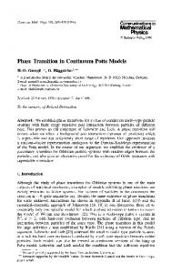
Fig. 1. The event that n{Xίy} = 0 and {x, y} is pivotal for "C(0)n G Φ 0" up to an x • y permutation. The solid lines show connections made by paths of occupied bonds, the square symbolizes the green set, and the dashed line represents the hypersurface which demarcates the cluster of the origin. Every bond which could connect sites on the inside of the surface to sites on the outside is unoccupied

b = {x, y}, and J(bL} = J(^y for the oriented bonds, b = (x, y). (In unoriented models, the latter couplings are identically zero.) Suppose that the unoriented bond b0 is unoccupied and pivotal for the origin being connected to the green set. Then the origin is connected to precisely one of the two sites of b0, the other site is connected to the green set and the cluster of the origin is free of green sites (see Fig. 1). If the bond b0 = (x, y) is oriented but otherwise as above, then we see that the same line of reasoning applies. Moreover, in this situation we know that x is the site to which the origin is connected. In light of these considerations, (3.3) can be rewritten as dMT

±=

Op

Σ x,yeAL

ProbL(x e C(0), C(0)nG = 0, C(y)r\G Φ 0) [J(£>y + J^J . (3.4)

Partitioning the events on the right-hand side of (3.4) according to the cluster of the origin, we obtain - = Σ

dβ

=

Σ

Σ ProbL(^ - C(0), x e C(0),

Σ

x,yeΛL A'.xeA

(3.5)

If y is in AL\A, then CAlλA(y) is the cluster of sites to which y is connected by a path of occupied bonds none of whose sites lies in A. For y not in AL\A, CΛlλA(y) is defined to be the empty set. The second equality in (3.5) is obtained by noting that a consequence of y lying outside of C(0) [since y is connected to G and C(0) contains no green sites] is that the path connecting y to G cannot make use of any bond having a site in C(0). In the terminology of [8], C(0) is a self-determined random subset of AL. Selfdetermined sets are often employed in the analysis of percolation models because they possess a locality property reminiscent of the nonanticipatory feature of stopping times in Markov processes and martingales. We make use of this property in the following way. Since all of the bonds which permit connections

Sharpness of Percolation Transitions

503

from sites in C(0) to sites out of C(0) are unoccupied, the cluster does not connect to the remainder of AL. Thus the distribution of bonds having no sites in A is unchanged when conditioned on the event "A = C(Q)" For this reason, (3.5) becomes

=

Σ

Σ

x,yeΛL A xeA

Clearly, the probability that y is connected to the green set in AL\A is bounded above by the probability that y is connected to the green set in all of AL9 i.e., by the finite volume order parameter. Thus, performing the summation over the sets A in the above expression, we have op

Σ ProbL(xeC(0), C(0)nG = 0) £ [4^ + 4L-U XQ obeying

1)

M\0

2)

M T"^00

as as

/z\0, /ZN

(4.6)

°'

and 3)

M^h

where α,θe(0, oo) and f

ah

+M/(M) + αM1+θ

an

,

(4.8)

satisfies

i)

0^/(M)0

as

(4.9)

M\0,

(4.10)

and (in)

dM0, and χL(β, h) — > χ(β, h) .

ML(β,h)—^M(β9h) L->oo

L-+OO

Proposition A.2. (i) M is a continuous function of β for h>0 and β^O and - in the unoriented case - also for h = Q and βή=βH. (ii) In finite range models, M is analytic in β for h>0. Both propositions make use of the following two estimates on Pn(β). Lemma A.3. For every L, ProbL(|C(0)| = rc,

where diam^4 = max{||x — y\\: x,yeA} and, for notational convenience, distances are measured using the £ ^ norm: ||x|| =max{|x i |: i= 1, ...,d}. The same bound is also satisfied (for noo, uniformly in L and uniformly on compacta in β. Proof. Suppose that in a given configuration the cluster of the origin contains exactly n sites. By disregarding occupied bonds which contribute to loops in this cluster it is possible to reduce the bond set of the cluster to a spanning tree of n — 1 bonds. If the diameter of the cluster is at least D then some bond in the tree must have length at least D/(n—ί). Thus there must be a (nonrepeating) walk along the spanning bonds which starts at the origin, proceeds along bonds in the allowed direction(s) and reaches this long bond in n—1 steps or less. So ProbL(|C(0) = w, diamC(O)^D) ^ Y Y (Σ ProbLK = 1)} k=ί i=ί\bi

Σ

Jbk: H x k - i - X f e l l ^ D / O i - l )

ProbLK = 1) , (A.2)

524

M. Aizenman and D. J. Barsky

where the bond b^ is either the unoriented bond {0, x x } or the oriented bond (0, x j and the succeeding bonds bi are either of the form {x^^xj or (x^^x,.). Using x 1 — e~ ^x, we replace (A.2) with ProbL(|C(0)| = n, diamC(0) ^D)

g /? V Osμ(L)l)fe ~ 1 fc=l

Σ

*fc: l l * f c - ι - x k | | ^ D / ( « - l )

(4?*+4L-U - (A 3)

(L)

In the first sum in (A.3) observe that |J | = |J| and in the second sum

Σ

\\x\\*D/(n-l)

4?»= L £ | | j c | | Σ £D

ΣJo.*+2i#£

Σ

Jo.* (A.4)

A similar bound holds for the oriented couplings. Combining (A.4) and its oriented analogue with (A.3) proves the bound (A.I). The full volume version of (A.I) is proved by repeating the argument which leads to (A.3). Π Lemma A.4. For every D, ProbL(|C(0)| = n, diamC(0) Prob(|C(0)| = n, diamC(0)9

(A.I)

and (A.8)

beB

The same decomposition can be used for the full volume probability of the above event where the only changes in (A.6)-{A.8) are the removal of the "L" subscripts and superscripts and, in (A.7), the relaxation of "yeΛL\A" to "ye!L\A" Upon considering the ratio of the infinite products EL and E, one finds

[

y*ΪΪAA V*o

y

J

which implies

(A.9)

Sharpness of Percolation Transitions

525

Note that the right-hand side of (A.9) tends to one (uniformly on compacta in β) as L-κx). Because there are only a finite number of factors in the products FL and F9 and since J(bL} ^>Jb as L-»oo for each beB, FL-+F. Thus EL(A) - FL(B)-^E(A) F(B) as L-»oo. This proves the lemma, since there are only a fixed number of pairs (A, B) which make a positive contribution to the sum in (A.9). Π The following result is not only the heart of the proofs of Propositions A.I and A.2(i), but it also may be of independent interest. Lemma A.5. Let n be finite. Then (i) lim P(n\β) = Pn(β) and the convergence is uniform on compacta in β, and «->00

(ii) Pn(β) is continuous in β. Proof. For both statements we use the decomposition p(V(β) = ProbL(|C(0)| - n, diam C(0) < D) + ProbL(|C(0)| - n, diam C(0) ^ D). (A.10) By Lemma A.3 the second term can be made arbitrarily small; by choosing D large enough, and using Lemma A.4, we see that the first term in (A. 10) has the desired convergence and continuity properties. Π Proof of Proposition A.I. In light of Lemma A.5(i), this is just a simple application of the Dominated Convergence Theorem. Π Proof of Proposition A.2. (i) By Lemma A.5(ii), M(β, h) is continuous in β whenever h is positive. For the unoriented h = 0 case, see [18]. (ii) This result is well-known in percolation theory (see [23]). The proof is based on the observation that for each finite n we may write Pn as a polynomial with nonnegative coefficients in the variables pb = Prob(nb = 1) and qb = 1 — pb. Once Pn is written in this form, bounds on all of its derivatives are easily obtained and analyticity of M(β, h) is not hard to show. Π Acknowledgements. We wish to thank C. Newman, J. Frδhlich, A. Sokal, and J. and L. Chayes for useful discussions on their results on topics related to this work. We would like to thank M. Beals for his comments on earlier drafts of this paper and J. Lebowitz, M. Bramson, and R. Schonmann for stimulating our interest in the contact process.

References 1. Kesten, H.: The critical probability of bond percolation on the square lattice equals 1/2. Commun. Math. Phys. 74, 41-59 (1980) 2. Russo, L.: On the critical percolation probabilities. Z. Wahrscheinlichkeitstheor. Verw. Geb. 56, 229-237 (1981) 3. Aizenman, M., Newman, C.M.: Discontinuity of the percolation density in one-dimensional l/|x-y| 2 percolation models. Commun. Math. Phys. 107, 611-647 (1986) 4. Aizenman, M., Chayes, J.T., Chayes, L., Imbrie, J., Newman, C.M.: An intermediate phase with slow decay of correlations in one-dimensional l/|x — y\2 Ising and Potts models (in preparation)

526

M. Aizenman and D. J. Barsky

5. Aizenman, M.: Contribution in: Statistical physics and dynamical systems (Proceedings Kόsheg 1984). Fritz, J., Jaffe, A., Szasz, D. (eds.). Boston: Birkhauser 1985 ά 6. Chayes, J.T., Chayes, L.: Critical points and intermediate phases on wedges of TL . J. Phys. A (to appear) 7. Hammersley, J.M.: Percolation processes. Lower bounds for the critical probability. Ann. Math. Statist. 28, 790-795 (1957) 8. Aizenman, M., Newman, C.M.: Tree graph inequalities and critical behavior in percolation models. J. Stat. Phys. 36, 107-143 (1984) s 9. Newman, C.M., Schulman, L.S.: One-dimensional l/|y — ί\ percolation models: The existence of a transition for s^2. Commun. Math. Phys. 104, 547-571 (1986) 10. Griffiths, R.B., Hurst, C.A., Sherman, S.: Concavity of magnetization of an Ising ferromagnet in a positive external field. J. Math. Phys. 11, 790-795 (1970) 11. Newman, C.M.: Shock waves and mean field bounds. Concavity and analyticity of the magnetization at low temperature. Appendix to contribution in Proceedings of the SIAM workshop on multiphase flow, G. Papanicolau (ed.) (to appear) 12. Aizenman, M., Fernandez, R.: On the critical behavior of the magnetization in highdimensional Ising models. J. Stat. Phys. 44, 393-454 (1986) 13. Harris, A.B., Lubensky, T.C., Holcomb, W.K., Dasgupta, C: Renormalization group approach to percolation problems. Phys. Rev. Lett. 35, 327-330 (1975) 14. Chayes, J.T., Chayes, L.: An inequality for the infinite cluster density in Bernoulli percolation. Phys. Rev. Lett. 56, 1619-1622 (1986) 15. Frδhlich, J., Sokal, A.D.: The random walk representation of classical spin systems and correlation inequalities. III. Nonzero magnetic field (in preparation) 16. Fernandez, R., Frδhlich, J., Sokal, A.D.: Random-walk models and random-walk representations of classical lattice spin systems (in preparation) 17. Griffiths, R.B.: Correlations in Ising ferromagnets. II. External magnetic fields. J. Math. Phys. 8, 484-489 (1967) 18. Aizenman, M., Kesten, H., Newman, C.M.: Uniqueness of the infinite cluster and continuity of connectivity functions for short and long range percolation. Submitted to Commun. Math. Phys. 19. van den Berg, J., Kesten, H.: Inequalities with applications to percolation and reliability. J. Appl. Probab. 22, 556-569 (1985) 20. Kesten, H.: Percolation theory for mathematicians. Boston: Birkhauser 1982 21. Griffeath, D.: The basic contact process. Stochastic Processes Appl. 11, 151-185 (1981) 22. Aizenman, M., Barsky, D.J., Fernandez, R.: The phase transition in a general class of Isingtype models in sharp. Submitted to J. Stat. Phys. 23. Chayes, J.T., Chayes, L., Newman, CM.: Bernoulli percolation above threshold: an invasion percolation analysis. Ann. Probab. (to appear)

Communicated by J. Frδhlich

Received September 28, 1986; in revised form October 24, 1986

Note added in proof. After submitting the manuscript we learned that the equality of pτ and pH was also proven, for finite range models, by Menshikov, M. V., Molchanov, S. A., Sidovenko, S.F. (in press), by means of an independent and somewhat different argument.