Abstract. Many existing rate control schemes in the literature consider spatial quality only. As a result, this may introduce a large distortion variation over frames ...
PID-based Real-time Rate Control Chi-Wah Wong*, Oscar C. Au, Hong-Kwai Lam Hong Kong Univ. of Science and Technology, Clear Water Bay, Hong Kong, China Email: {dickywcw*, eeau, eekwai}@ust.hk Abstract Many existing rate control schemes in the literature consider spatial quality only. As a result, this may introduce a large distortion variation over frames that human is sensitive to. In fact, human is also sensitive to temporal quality. In this work, we design the real-time rate control based on PID controller to have better tradeoff between spatial and temporal quality. From different estimated number of bits of frames and buffer status, different target bits of each frame are used in order to reduce flickering effect (smaller distortion variation) which is one factor to affect temporal quality. The experimental results suggest that our scheme can obtain more consistent quality while keeping high spatial quality. 1. Introduction Standard video systems, such as H.26X and MPEG, exploit the spatial, temporal and statistical redundancies in the source video. Since the level of redundancy changes from frame to frame, the number of bits per frame is variable, even if the same quantization parameters are used for all frames. Therefore, a buffer is required to smooth out the variable video output rate and provide a constant video output rate. The rate control is used to prevent the buffer from over-flowing (resulting in frame skipping) or/and under-flowing (resulting in low channel utilization) in order to achieve good video quality. For real-time video communications such as video conferencing, it is more challenging as the rate control is required to satisfy the low-delay constraints, especially in low bit rate channels. Controlling bit rate only is not enough to achieve good video quality. Therefore, the distortion should be considered while doing the rate control [1], [5], [6], [7], [8]. This can be done by minimizing the mean-square error (MSE) or maximum distortion. This work minimizes MSE. Using Lagrange optimization, we minimize the distortion subject to the target bit constraint in our model and obtain formulas that indicate how to choose the quantization parameters. Many existing rate control schemes (e.g. [1], [5], [6], [8]) consider spatial quality only. Some minimize average distortion or maximum distortion. In fact, temporal quality is also important. Motion jerkiness and flickering are two main factors to affect temporal quality. Good temporal quality should have fixed frame rate (>some threshold frame rate) to avoid motion jerkiness or/and have small distortion variation to minimize the flickering effect. Some recent research does rate control to achieve better tradeoff between spatial and temporal quality by controlling quantization step size and frame rate. However, controlling frame rate is not good to have better temporal quality due
0-7803-8603-5/04/$20.00 ©2004 IEEE.
to motion jerkiness. Human can be able to notice the sudden change of frame rate. This means that changing frame rate is not a good idea to have better temporal quality. In addition, a frame-rate overhead should be specified into a header. There is some other ways to achieve better temporal quality. One way can be using different number of target bits of each frame to be allocated at fixed frame rate such that distortion variation is reduced. This task is very challenging in real-time communications because this kind of communications needs low-delay requirement and buffer status should not be so large. In this work, we present a PID-based rate control scheme for H.26X encoders in real-time video communications. This work focuses on doing rate control for inter-coded frames (i.e. P-frame), which is used mostly in low-delay video communications. We first introduce a PID controller, which is a controller with three terms in which the output of the controller is the sum of a proportional term, an integrating term, and a differentiating term, with an adjustable gain for each term. The popularity of PID controllers can be attributed partly to their robust performance in a wide range of operating conditions and partly to their functional simplicity, which allows engineers to operate them in a simple, straightforward manner. By using PID method, smaller distortion variance can be achieved in our proposed method. Therefore, flickering effect can be reduced (small distortion variation) and motion jerkiness can be avoided (fixed frame rate > threshold). This paper is organized as follows. In the following section, we describe PID controllers. In section 3, we describe the error function e(t) from PID controllers. In section 4, our proposed rate control scheme is described. In section 5, the experiments are conducted to evaluate the performance. Finally, the conclusion is made. 2. PID Controller PID controller is a controller, which uses proportional (P), integral (I) and derivative (D) controls to obtain a desired response.
R
e -
m Controller
Y Plant
Figure 1: An overall system with a plant and a controller Figure 1 shows an overall system with a plant to be
controlled and a general controller to be designed to control the overall system behavior. Designing a controller is important to control the system. PID controller is one kind of popular controllers to control our desired system response due to their robust performance in a wide range of operating conditions and their functional simplicity.
The final PID equation with Kcr = 0.7407, Pcr=2/F and Δt = 1/F (F: frame rate) is
The PID function can be expressed as follows:
It is observed that M is the function of e(t). When e(t) is known from t0 to t, M can be calculated. The following section will describe how to define the error function e(t).
1 M = K p e(t ) + T i
t
∫ e(t )dt + T
d
t0
de(t ) dt
(1)
where e(t) is the error function, Kp is the proportional gain, Ti is the integration factor and Td is the derivative factor.
i (t ) M = 0.7407 0.6e(t ) + 0.6∑ e(i ) + 0.15∆e(t ) i =i0
3. Error Function e(t) In TMN8 rate control [1], a quadratic model is used. The rate model per MB is
The PID corresponding transfer function is:
R = A( K
1 + Td s E (s ) (2) M (s ) = K p 1 + T s i e(t) is the difference between the desired input value, R and the actual output, Y. e(t) will be sent to the PID controller and the controller calculates both the derivative and the integral of this error function to control the system. From Eq.(1), there are three terms. The first is a proportional term, which is a function of time t only. It can be said that this term gives current error information. e(t) = 0 when no current error occurs. The second is an integral term, which is a function of time from t0 to t. This term gives past error information. This means that the error’s trend is known based on past error function (from t0 to t).
t
∫ e(t )dt = 0
when no accumulated error occurs.
t0
The last is a derivative term, which is a derivative function with respect to t. This gives slope of the error curve at time t. Slope information is likely to give future error function. de(t)/ds = 0 when previous and current errors are the same. Since the equation M has three terms, M can be likely to have current, past and future error information. In case of discrete case, the PID equation becomes M = K p e(t ) +
K p ∆t Ti
i (t )
∑ e(i) + K
T
p d
i =i0
∆e(t ) ∆t
(3)
According to Ziegler-Nichols rules, the PID controller is tuned. The settings are Kp = 0.6Kcr, Ti = 0.5Pcr and Td = 0.125Pcr. After substituting these settings, the PID equation becomes M = 0.6 K cr e(t ) +
1.2 K cr ∆t Pcr
i (t )
∑ e(i) + i = i0
0.075 K cr Pcr ∆e(t ) ∆t
(4)
In order to make the weighting terms sum up to 1, 0.6 K cr +
1.2 K cr ∆t 0.075K cr Pcr + =1 Pcr ∆t
(5)
(6)
σ i2 Qi2
+ C)
(7)
where Qi is the optimal quantization step size of the i-th macroblock (MB), A is the number of pixels in a MB, K is a model parameter, σi is the standard deviation of the prediction error of the i-th MB, and C is the overhead rate. Based on this quadratic model, the error function e(t) can be expressed as the difference between estimated number of bits of current and previous frames. N N σ2 σ2 e(t ) = A( K i2 + C ) − A( K i2 + C ) Q Q i i i =1 curr i =1 prev AK ≈ S − S curr prev 2 Q prev
∑
∑
(
(8)
)
where N is the number of MBs of each frame, curr is the current frame, prev is the previous frame, Qprev is the average quantization step size of the previous frame, N N S curr = ∑ σ i2 and S prev = ∑ σ i2 i =1 curr i =1 prev If e(t) > 0, residue energy is larger in the current frame. This means that the current frame needs more bits by using average previous quantization compared with the previous frame. If it is assumed that distortion is Q2/12 (i.e. uniform quantizer for uniform distribution), it should put more bits on frames with higher residue energy in order to have similar distortion. Some real-time rate control schemes (e.g. TMN8) use similar target bit of each frame. It is known that more bits should be given to some frames with larger residue energy whereas fewer bits should be given to some frames with smaller residue energy. Therefore, target bits of each frame should be changed more such that more bits can be allocated to some bit-demanding frames. e(t) acts as a good indicator to determine whether the current frame needs more or less target bits. By doing this, distortion variation is smaller. Let’s use P-term as example. Frames with larger residue energy (P>0) use more bits and distortion becomes smaller. On the other hand, frames with smaller residue energy (P