Piece Selection Algorithm for Layered Video Streaming in P2P Networks Tibor Szkaliczki a,1,2, Michael Eberhard b,3, Hermann Hellwagner b,4 and L´aszl´o Szobonya a,5 a
eLearning Department, Computer and Automation Research Institute of the Hungarian Academy of Sciences Budapest, Hungary b
Institute of Information Technology Klagenfurt University Klagenfurt, Austria
Abstract This paper introduces the piece selection problem that arises when streaming layered video content over peer-to-peer networks. The piece selection algorithm decides periodically which pieces to request from other peers (network nodes) for download. The main goal of the piece selection algorithm is to provide the best possible quality for the available bandwidth. Our recommended solution approaches are related to the typical problems and solutions in the knapsack problem. Keywords: streaming, layered video, knapsack problem
1
Partial support of the Hungarian National Science Fund and the National Office for Research and Technology (Grant No. OTKA 67651) is gratefully acknowledged. 2 Email:
[email protected] 3 Email:
[email protected] 4 Email:
[email protected] 5 Email:
[email protected]
1
Introduction
Nowadays peer-to-peer (P2P) networks provide a very popular alternative to the traditional distribution of content through servers. Especially with the increasing demand for high definition multimedia content, the bandwidth required from the distribution servers is constantly increasing. P2P networks provide a good alternative, as the content is distributed from the users to other users during consumption. Another requirement on content distribution today is the provision of content in different qualities. As the users want to consume the content on various devices like HD TV sets, laptops, or mobile phones, the content has to be provided in a quality suitable for the end devices’ displays as well as their computational capabilities. A possibility to provide these different qualities within one bitstream is provided by scalable video codecs like the Scalable Video Coding (SVC) extensions of the Advanced Video Coding (AVC) standard [6]. To distribute scalable content over Bittorrent-based P2P networks, the content needs to be split up into pieces. For scalable content, each piece belongs not only to a specific time slot, but also to a specific layer. It is important to note that the higher layers of scalable codecs, which offer better quality, depend on lower layers for the decoding process. Thus, a piece belonging to a higher layer is only useful if also the piece from the lower layer it depends on is available. During the download process, this layer dependency as well as the availability of the pieces on multiple neighbour peers needs to be considered. When the scalable content is distributed in a P2P network, the questions when and which pieces to download to receive the content in the desired quality provides a challenging task. When non-scalable content is downloaded over P2P networks, the piece selection algorithm, which selects the pieces for download from other peers, is rather straightforward: the pieces with more urgent deadlines are downloaded first and with higher priority, to ensure that the playback of the multimedia content never stops. However, when considering scalable content, the piece selection process is becoming more complicated. On the one hand, the user wants to receive the best possible quality for the available bandwidth, but on the other hand an undisturbed playback of the content should be guaranteed. Thus, the piece selection algorithm needs to find the best trade-off between downloading the best possible quality while still ensuring that all the pieces are received in time. Another requirement to the piece selection algorithm is that frequent quality switches should be avoided, as subjective quality measurements [7] have shown that users prefer to consume the content at a constant lower quality than to consume the
t-1
t
t+1 t+2 t+3 t+4 t+5 t+6
EL3
0.0
0.0
0.0
0.0
0.0
0.0
0.0
0.0
EL2
1.0
1.0
0.8
0.0
0.0
0.0
0.0
0.0
EL1
1.0
1.0
1.0
0.5
0.0
0.0
0.0
0.0
BL
1.0
1.0
1.0
0.8
0.2
0.0
0.0
0.0
Fig. 1. Sliding Window
content with frequently switching higher quality. The piece selection algorithm works on a so-called sliding window. The sliding window is illustrated in Fig. 1. In the sliding window shown in Fig. 1, the piece selection algorithm has to decide which pieces should be downloaded for the upcoming time slots t + 1 to t + 4. The numbers in the cells indicate the download progress, where 1.0 indicates a successfully finished download and 0.0 indicates that the download has not yet started. During previous decision points, the download for EL2 of t+1, BL and EL1 for t+2, and BL for t+3 has already been started and is still in progress. At the current decision point, the algorithm has to decide which pieces to download first: the base layer pieces for t + 4 and t + 5 (to ensure undisturbed playback), the EL2 piece for t + 2 (to ensure that the current quality is kept), or even the EL3 piece for t + 1 (if there is enough bandwidth available). In addition to the decision which pieces to download, a neighbour peer has to be assigned for each piece for the download process. This decision is taken based on the priority and size of the selected piece as well as based on the estimated provided download bandwidths of the neighbour peers.
2
The Problem Model of Piece Selection
In this section, some notations are introduced for the specification of the piece selection problem and the problem is defined formally. Let m and n denote the number of columns (time slots) and rows (layers) in the sliding window, respectively. Let li denote the ith layer of the stream (i = 0..n − 1). Let Pi,j denote the piece of the stream of layer lj for the ith time slot in the sliding window. Let the utility of piece Pi,j be denoted by ui,j . The calculation of the utility of a piece is quite complicated and is out of the scope of the present paper. Let the cost (size) of the piece be denoted by ci,j . The cost of the piece is a constant piece packet size c multiplied by the
number of piece packets needed for one time slot at layer lj . Typically, the cost of the piece does not depend on the time slot (i.e., is independent from i). xi,j shows whether Pi,j is requested by the client from any node. There is a limited buffer size S on the client. Maximize P The total utility of the selected pieces: ui,j · xi,j Subject to X (1) ci,j · xi,j ≤ S i,j
(2)
(xi,j = 1 ∧ j > 0) ⇒ (xi,j 0 = 1) ∀j 0 < j
(3)
(xi,j = 1 ∧ i > 1) ⇒ (xi−1,j = 1)
(4)
xi ∈ {0, 1}
The first constraint expresses the limit on the total size of the pieces. The dependency between the pieces is described in constraints 2 and 3. Constraint 2 describes that if a piece is selected then all pieces in layers in lower layers are also selected. In order to avoid frequent quality switches, constraint 3 ensures that a piece is selected only if the piece in the preceding time slot in the same layer is also selected for download.
3
Algorithms to Solve the Problem
The piece selection process tries to maximize the utility of the selected pieces without surpassing the available resource limit. This problem is similar to the Knapsack problem (its 0-1 version when at most one sample can occur from each item). The only but relevant difference is that a piece can be selected only if the pieces it depends on are also downloaded. The running time is critical because the piece selection is executed repeatedly at the decision point of each time slot. 3.1 Greedy Approximation Algorithm For the piece selection problem, the greedy solution of the knapsack problem [3] offers a fast solution: select the pieces for which the value and size ratio is the highest among the pieces whose size is not larger than the available resource. We may restrict the selection to the pieces for which the pieces they depend on are already selected or their download has been started before. This greedy selection can be repeated as long as there are still enough resources for the download of one complete piece available. This approximation algorithm
runs fast but the solution of the algorithm may be far from optimal in the worst case. 3.2 Dynamic Programming 1 There is well-known efficient solution using dynamic programming if the cost values are integers [1]. Applying it to our case, the algorithm proceeds on each possible total cost values and on the available pieces and calculates the maximum utility in a step-by-step way that can be achieved using at most the current cost value and the pieces up to the current piece. This solution of the general knapsack problem does not consider the constraints among the pieces, i.e., that the piece is useful only if the pieces it depends on (pieces of lower layers or pieces in the preceding timeslot) are also selected. However, if Eq. 5 holds then a piece is selected in the optimal solution only if all pieces it depends on are also selected. This can be proved easily in an indirect way: let us assume that there is a piece that is not included in the solution although a depending piece is selected. Let us add this piece to the solution and omit the depending piece. The size constraints is still fulfilled while the utility is increased, which contradicts the optimality. Therefore, the above dynamic programming solution can be used if the value of the utilities and sizes harmonise with the dependency among the pieces. (5)
(Pi2 ,j2 depends on Pi1 ,j1 ) ⇒ (ui1 ,j1 > ui2 ,j2 ∧ ci1 ,j1 ≤ ci2 ,j2 )
The running time is O(S · m · n) (the cost values go from 0 to S and the number of different pieces is m · n). It is a pseudo-polynomial time algorithm because the value S is exponential in the numeric representation of S in the input. 3.3 Dynamic Programming 2 Now, let us consider a more general algorithm that can be used in the case when the relative values of the utilities and sizes of different pieces are independent from the dependency between the pieces. We apply the dynamic programming approach again, but in this case the dependency between pieces in the neighbouring timeslots has to be considered in an explicit way in the steps of the algorithm. Let us sort the pieces according to the time slots and the pieces in the same time slot according to the layer in increasing order. Let U(i, j, k), (i = 1..m, j = 0..n, k = 0..S) denote the maximum utility that can be attained with size less than or equal to k using pieces Pi0 ,j 0 up to piece Pi,j−1 (i.e. (i0 < i) ∨ (i0 = i ∧ j 0 < j)) if j > 0 and piece Pi,j is certainly selected or
using pieces from the time slots before the ith one if j = 0. Although the dynamic programming solutions to the knapsack problem usually do not require that the current item is definitely included into the partial solution represented by the state variable, P (i, j) has to be included into the optimal partial solutions represented by U(i, j, C) because of the constraints on dependency between the pieces. Auxiliary variables are introduced to store cumulative values of utilities and sizes of the piece and depends on P all of the pieces it P in the same timeslot, respectively: Ci,j = jj 0 =0 ci,j 0 and Ui,j = jj 0 =0 ui,j 0 if j > 0 otherwise Ci,0 = 0, Ui,0 = 0. (6) (7)
U(i, j, C) = 0 if C < Ci,j , U(1, j, C) = U1,j
i = 1..m, j = 0..n, C = 0..S
if C ≥ Ci,j ,
j = 0..n, C = 0..S
(8) U(i, j, C) = max (Ui,j + U(i − 1, j 0 , C − Ci,j )) 0 j =j..n
if C ≥ Ci,j , i = 2..m, j = 0..n, C = 0..S Eq. 6 claims that the achievable utility is 0 if the size limit C is less than the overall sizes of the piece Pi,j and of the pieces it depends on. Processing the first time slot is easy, in this case the achievable utility is the cumulative utility of the piece if its cumulative size is below the size limit (Eq. 7). In the general case as shown in Eq. 8, piece Pi,j can be selected only if piece Pi−1,j is also selected. In the first time slot (i = 1), U(i, j, C) = 0 implies that U(i, j 0 , C) is also 0 for each j 0 > j (Eqs. 6 and 7). Eq. 8 ensures that this condition is fulfilled for the other time slots as well and if U(i, j, C) = 0 then U(i, j + 1, C) is also equals to 0. Now U(i, j, C) can be calculated for each possible i, j and C values based on the recursive equations. The maximum total utility is maxj U(m, j, S). Similarly to the dynamic programming solution of the general knapsack problem, the selection belonging to the maximum utility can be found by backtracking the U(i, j, k) array. The running time is O(S · n · m2 ). 3.4 Multiple-choice Multidimensional Knapsack Problem The dependency of the pieces from lower layers can be omitted if we consider the multiple-choice knapsack problem (MCKP). In this case, there are several groups of items and it is enough to choose only one item from each group. In our problem, one item represents the piece sequence from the lowest layer piece which is still not downloaded to any higher layer piece. The items belonging to the same time slot form a group. In this case, we have to select at most one item for each time slot.
Another generalisation of the knapsack problem is the multidimensional knapsack problem. In this case, there are several knapsacks (resources) each of them with limited capacity. The resource needs of the items can be described as a vector because an item needs several resources at the same time. The aim is to optimise the value of the selected items while none of the resources is overloaded. The main advantage of applying the multidimensional knapsack problem is that it can consider not only the buffer size but simultaneously other resources as well, e.g., the bandwidth capacities on the routes from the peers to the client. Several heuristic algorithms have been proposed for the multiple-choice multidimensional knapsack problem (MMKP) in the literature. [4] gives a good overview on them. [5] applied the MMKP for an adaptive multimedia problem. This approach proved to be an efficient method to solve problems like quality adaptation, admission control and integrated resource management. A heuristic method and an exact branch-and-bound method were introduced as well for checking the results. [2] applied the MCKP to select sources for different video layers. The approaches based on MCKP can deal well with the dependency between the layers but they do not consider the dependency between pieces in the subsequent time slots.
4
Conclusion
In this paper we recommended solutions to the piece selection problem appearing in the area of multimedia. We found that the problem is in close relation to the knapsack problem and we adapted the typical solution methods of this combinatorial optimisation problem to our case. The efficiency of the different methods varies and some of them need additional constraints. Table 1. compares the presented algorithms w.r.t the additional conditions they require to solve the piece selection problem. Applying the presented approaches to an adaptive video streaming system yields a better multimedia experience for the user. Solution methods for MCKP have to be adapted to our problem by considering the dependency between the subsequent time slots. Experiments will be performed to appropriately adapt the methods to the practical problem. It should be again noted that the pieces selected during the piece selection process are downloaded from a number of different neighbour peers that provide some or even all of the selected pieces. Thus, we are also developing algorithms to the peer selection process. The peer selection is based on the output of the piece selection and it assigns a peer to every selected piece considering the limited bandwidths to
Table 1 Comparision of the examined solution approaches
Method
Special condition
Exact/approximating
Greedy
none
possible large error
Dyn. Prog 1
integer piece sizes and Cond. 5
exact
Dyn. Prog 2
integer piece sizes
exact
MCKP based
without Cond. 3
various methods
the peers serving the pieces.
References [1] Andonov, R., Poirriez, V. and Rajopadhye, S., Unbounded knapsack problem: Dynamic programming revisited, European Journal of Operational Research 123, Issue 2, (2000), Pages 394-407 [2] Cheok, L-T. and Eleftheriadis, A. Operations Research Approach Towards Layered Multi-Source Video Delivery, in Picture Coding Symposium 2004, (San Francisco, CA, USA), Dec. 2004. [3] Dantzig, G. B., DiscreteVariable Extremum Problems, Operations Research, 5, (1957), 266277. [4] Han, B., Leblet J., and Simon, G., Hard multidimensional multiple choice knapsack problems, an empirical study, Computers and Operations Research, 37, 1, January 2010, Pages 172-181 [5] Khan, S., Li, K.F., Manning, E.G., Akbar, M., Solving the knapsack problem for adaptive multimedia, Studia Informatica (special issue on Cutting, Packing and Knapsacking Problems) 2 (1), (2003), pp. 157-178 [6] Schwarz, H., Marpe, D., Wiegand, T., Overview of the Scalable Video Coding Extension of the H.264/AVC Standard, IEEE Trans. on CSVT, 17, no. 9, (2007), pp. 1103-1120. [7] Zink, M., Kuenzel, O., Schmitt, J., Steinmetz, R., Subjective Impression of Variations in Layer Encoded Videos, IWQoS 2003: 137-154.