Piecewise rotations: symbolic dynamics
arXiv:1306.6150v4 [math.DS] 2 Jul 2014
Nicolas B´edaride∗
Idrissa Kabor´e†
ABSTRACT We consider piecewise rotations as studied in [6], [12] and [10]. If the angle belongs to the set { π2 , π3 , π6 , π4 , π5 } we give a complete description of the symbolic dynamics of this map, no matter wheter the map is bijective, non-injective or non-surjective.
1
Introduction
In this paper we consider the dynamics of a piecewise isometry. A piecewise isometry in Rn is defined in the following way: consider a finite set of hyperplanes; the complement X of their union has several connected components. The piecewise isometry is a map T from X to Rn which is locally defined on each connected component as the restriction of an isometry of Rn . Now consider the pre-images of the union of the hyperplanes by T : it is a set of measure zero. Thus almost every point of X has an (infinite) orbit under T and we will study this dynamical system (X, T ). The class of such maps has been well studied in dimension 1 with primary example given by interval exchange maps: in this case the map is bijective, equal to the identity outside of a compact interval, and the isometries which locally define T are translations. The case of the dimension 2 has first been considered ten years ago in the paper [1]. Since them, different examples have been worked out in order to exhibit different types of behaviors, see for example [11] or [4]. The first general result has been obtained by Buzzi who proved that every piecewise isometry has zero entropy, see [7]. An important class of piecewise isometries is the outer billiard. Around this map a lot of developments in recent years takes place, in particular with the work of Schwartz: [15], [16], ∗
Aix Marseille Universit´e, CNRS, Centrale Marseille, I2M, UMR 7373, 13453 Marseille, France. Email:
[email protected] † Universit´e Polytechnique de Bobo Dioulasso,01 PB 1091, Bobo-Dioulasso, Burkina Faso. Email:
[email protected]
1
[17] and [18]. He describes the first example of a piecewise isometry of the plane with an unbounded orbit. Here we study another example, which was introduced in [6] by Boshernitzan and Goetz. This map is called a piecewise rotation. Up to date it is perhaps the piecewise isometry which has been studied the most, see [12] and [10]. Consider a line in the plane (assumed to be the real axis R), two points P0 , P1 outside the line and an angle θ ∈ [0, 2π). The map is locally defined on each half plane (defined by the line) by a rotation around Pi with angle θ. The phase space of the map can be described with two parameters: one for the angle and one which measures the relative positions of the centers. If the middle of the segment [P0 , P1 ] belongs to the line, then this parameter is null and the map is called symmetric. Among the positions of the centers of rotations this map can be bijective, non injective, non surjective. In [6] Boshernitzan and Goetz show that in the two last cases the map is either globally attractive or globally repulsive. In the bijective case, Goetz and Quas have shown that for a rational angle every orbit is bounded, see [12]. In order to prove this result they introduce symbolic dynamics for this map. They define the notion of rotationally coded points, which represent points which have the same symbolic coding as points under the action of a rotation of the fixed angle, centered at the origin. This notion is very useful to find periodic orbits, but it only works for maps close to the symmetric ones. In the irrational case, the previous authors and Cheung were able to give precise bounds on the density of periodic orbits, see [10]. In the present paper we want to give a precise description of the symbolic dynamics. We do not want to restrict to bijective cases or to symmetric cases inside the bijective case. Nevertheless we restrict our study to a finite family of angles. In the cases π5 , π4 we find some bounded orbits which are not periodic. Thus these orbits do not come from rotationally coded orbits. Our method of investigation is close to the one introduced in [9] for the outer billiard outside regular polygons. The main idea is to find a reasonable set, where we can consider the first return map and prove that it is conjugated to the initial map. This allows us to use substitutions in order to describe the language of the map. Of course, in most of the other cases, the approach is not so simple: we need to use different transformations before being able to find a good renormalisation, see Proposition 5.3 for a complete study of one particular case. It is not so surprising that the techniques in this case (for a rational angle) and for the outer billiard map are similar. In both cases the maps are related to piecewise translations defined on cones of the plane. Moreover,the proof that every orbit of the outer billiard is bounded for a special sort of polygons is close to the proof that every orbit is repulsive in the non-surjective case for 2
the piecewise rotation, see [8] for a review on outer billiard. Finally we can mention the work of Akiyama on some arithmetic problem which was solved by a dynamical method. In this work, he introduces a piecewise isometry close to the one studied here, see [2, 3]. The method is however different, since he obtains a result for any angle, but the description he gives is less precise. This work has been supported by the Agence Nationale de la Recherche – ANR-10-JCJC 01010.
2
Definition of a piecewise isometry and some background
Consider a line l in R2 , it splits the plane on two half-planes. Now we define a piecewise isometry T on R2 such that the restriction to each half-plane is given by a rotation. The two rotations are of the same angle with different centers, which may lay outside of the corresponding half-plane. We also assume that the centers of rotations are not on the line l. Without loss of generality we can identify the plane with the complex numbers C and the line with the real line R. Then if the centers have coordinates z0 , z1 , the map is given by: C \ R 7→ z
C\R ( 2iπθ e (z − z0 ) + z0 → T (z) = e2iπθ (z − z1 ) + z1
Im(z) > 0 Im(z) < 0
Remark 2.1. Every point z ∈ C has not a well defined orbit for T . Consider the set of complex numbers z such that there exists an integer n with T n z ∈ R. This set of points is called the set of discontinuity points, but it is of zero measure and we can ignore it. In the following we will only consider orbits of points outside this set. In [6] the authors prove the following theorem: Theorem 2.2 (Boshernitzan-Goetz). If T is non-injective then there exists a constant M > 0 such that for any integer n, |T n z| ≤ M for all sufficiently large positive integer n. If T is non-surjective, then there exists a constant M 0 > 0 such that lim |T n (z)| = ∞ for all z satisfying |z| ≥ M 0 . +∞
This results shows that the bounded orbits either accumulate or stay inside a compact set. The bijective case was not treated by this result, it has 3
been done by Goetz and Quas, see [12]. In the bijective case, the map can be written in an particularly easy way: ( e2iπθ (z + σ + 1) Im(z) > 0 T (z) = e2iπθ (z + σ − 1) Im(z) < 0 where σ is a real number. If σ = 0 the map is called a symmetric map. The parameter θ is called the angle of the map by a slight abuse of notation. In order to explain the results of Goetz-Quas we need to introduce some notions of symbolic dynamics, see [14]. Let A be a finite set called alphabet, a word is a finite string of elements in A, its length is the number of elements in the string. The set of all finite words over A is denoted A∗ . A (one sided) infinite sequence of elements of A, u = (un )n∈N , is called an infinite word. A word v0 . . . vk appears in u if there exists an integer i such that ui . . . ui+k+1 = v0 . . . vk . For an infinite word u, the language of u (respectively the language of length n) is the set of all words (respectively all words of length n) in A∗ which appear in u. We denote it by L(u) (respectively Ln (u)). Let P0 , P1 be the two half-planes bounded by the discontinuity line of T . Let φ : C 7→ {0; 1}N be the coding map where the image of a complex number z is given by φ(z) = (un )n∈N such that T n (z) ∈ Pun for all integer n. The image by the coding map of the points which have well defined orbit defines a language. For an infinite word u in this language, a cell is the set of points which are coded by this word: {z ∈ C, φ(z) = u}. Definition 2.3. A point z ∈ C is called a pq rationally coded point if there exists p, q ∈ N∗ with gcd (p, q) = 1 such that: • There exists y ∈ C such that Rn (y) ∈ / R for all integer n, where R : 2iπp q C → C is given by R(z) = e z. • For all integer n we have: Rn (y) ∈ Pun ⇐⇒ T n (z) ∈ Pun , where (un )n∈N = φ(z). The symbolic dynamics of a rationally coded point is the same as the dynamics of the point under the rotation R. Remark that such an orbit is periodic and thus its coding is easy to compute: the orbit of one point stays on a regular polygon with q vertices. If p = 1 then there are three orbits: one if q = 2k given by (0k 1k )ω and two for the case q = 2k + 1 given by (0k 1k+1 )ω , (0k+1 1k )ω . If p is bigger than one, we need to take a subsequence of these words made by an arithmetic progression of common difference p. Consider a rational number θ = dc , then define pq00 as the rational number: p0 = max{r ∈ Q, r < θ, q0 < d}. q0 4
We define the approximation sequence ( pqkk )k∈N as the irreducible fractions given by p0 + kc pk = . qk q0 + kd Then in [12], Goetz and Quas proved the existence of a lot of periodic orbits (with a precise coding) for the map T . Theorem 2.4 (Goetz-Quas). With preceding definitions: • If θ ∈ / Q, then T has rationally coded points in every neighborhood of infinity. • If θ = dc ∈ Q, then consider the approximation sequence ( pqkk )k∈N . If σ is sufficiently small, then – For all integer k, T has a
pk qk
rationally coded periodic point.
– If qk is odd, then there are two such orbits. – The cells associated to such an orbit (or two orbits) form a connected set which forms a ring. – If qi and qj have the same parity, then the corresponding cells are translated one from the other. Corollary 2.5. For a rational angle θ, all the orbits are bounded. Every ring is an invariant region. In the preceding theorem an important fact is that the parameter σ must be small. Thus the maps are closed to symmetric ones. The different forms of this map can be summarized in the following arrays: Bijective case Symmetric Non symmetric
3 3.1
Non bijective case Non injective Non surjective
Words and symbolic dynamics Substitutive language
A substitution σ is an application from an alphabet A to the set A∗ \ {ε} of nonempty finite words on A. It extends to a morphism of A∗ by concatenation, that is σ(uv) = σ(u)σ(v). In the following we will denote a substitution by an array which has on the first line the elements of the alphabet and on the second line their images by the substitution.
5
Figure 1: Cellular decomposition for the angle 18 .
Now we introduce the notion of substitutive language. Consider a finite set S of substitutions, and X a finite set of words. A substitutive language is the set of factors of an union of words of the form g(u) where g is a product of some substitutions of S and u is a finite word of X. A good way to represent it is to use a finite oriented graph such that the each edge is marked by a substitution of S and on each vertex is attached a finite union of words of X. We attach to each path on this graph a set of words by the following way: consider one edge marked by σ between the vertices A, B. Then we associate to this edge the set of words {σ(a), a ∈ A} ∪ {b ∈ B}. For a path obtained by concatenation of several edges we compose the substitutions. The set of paths on this graph defines the words of the language. In other terms, we start from a set of words and along the path we apply some substitutions to this set or to the set associated to the vertices in the path. A language is said to be substitutive if there exists a finite number of substitutions and a graph with edges marked by the substitutions such that the language is the set of factors of the words associated to all finite paths on the graph. By convention, if there is only one substitution, we will only draw one vertex labelled with a finite set of words. Example 3.1. For the following graph, if X is a set of finite words, the language is the set of factors of the words z ω where z belongs to Z defined by: [ Z= {σ3p ◦ σ2m ◦ σ1n (X)}. n,m,p∈N
6
σ2 σ1
X
σ2
X
σ3
σ3
X
The substitutive language will be usefull in the statement of the results. It already appears in the description of the language of the outer billiard outside a regular pentagon see [9], and in the study of S-adic systems, see [5] for a recent survey.
3.2
Induction and substitution
In this subsection we recall some usual facts about the relation between the coding of a map and the coding of the map obtained by an induction of the initial map on a subset. Let X be an open subset of Rd , and T a map from X to X. Assume there is a partition of X by the sets Ui , i = 1 . . . k, then consider the language LU obtained by the associated coding map. Now assume that the first return map of T on U1 , denoted by TU1 , is defined by: TU1 (x) = T nx (x), where nx is the smallest positive integer such that T n x belongs to U1 for x ∈ U1 . Consider the partition of U1 in which the return time nx is constant on each part of the partition. This partition is associated to a coding map for the map TU1 . We denote the associated language by LU1 . We denote the elements of the alphabets of the language of TU1 , T by the same letters. We will give conditions to describe the language of this first return map in terms of the initial language. If x is in one cell of the partition of U1 then denote by vi the finite word of length nx which codes the orbit T j x, j = 0 . . . nx − 1 where nx is the return time of x in U1 . By definition nx is constant for all x ∈ U1 . Now define the substitution αU1 by 1 ... k i αU1 (i) v1 . . . vk Lemma 3.2. • In general we have αU1 (LU1 ) ⊂ LU . • If the maps are defined for every set Ui , we have
[ i
7
αUi (LUi ) = LU .
• Assume there exists an isometry h between X and U1 which maps each Ui , i = 1 . . . k to one subset of TU1 such that for all x ∈ X we have h−1 ◦ TU1 ◦ h(x) = T (x). Then we have LU1 = LU . Moreover LU is stable by αU1 . The proof is classical and can be found in the litterature. If the hypothesis in the third statement is fulfilled we say that the map has a renormalisation or is self-similar. This lemma will be used in the different proofs in order to describe the language in terms of substitutions.
4
Results and overview of the paper
4.1
Statement
We consider the angles θ ∈ { 14 , 31 , 16 , 15 , 81 } and give a complete description of the symbolic dynamics in all the cases. Due to the formulation of the map T , the centers of rotations are the points e2iπθ (σ − 1) e2iπθ (σ + 1) , z1 = . (1) z0 = 1 − e2iπθ 1 − e2iπθ σ±1 The imaginary parts of the centers of rotations are equal to 2 tan . In all πθ our cases tan πθ is a positive number, thus the two centers of rotations define a periodic point of T if and only if σ ∈ [−1, 1]. Moreover, note that the cases σ < −1 and σ > 1 are equivalent since the two corresponding maps are conjugated to each other by the map z 7→ −z. Thus we can restrict the values of the parameter σ to the interval [0, +∞).
Theorem 4.1. We can describe the symbolic dynamics of a bijective piecewise rotation for the following angles : • If θ ∈ { 14 , 13 , 61 }, every orbit is periodic. • If θ ∈ { 15 , 18 }, every orbit is bounded but some are non periodic. • For non symmetric cases, the dynamics is the same for all value of a rational number σ ∈ (0, 1). In all the cases the language is substitutive. The proof for the symmetric case is made in Propositions 5.1, 5.3. For the non symmetric cases see Section 6, where the role of the parameter σ is shown. 8
For the non bijective piecewise rotations we study the dynamics related to the compact set made of points of bounded orbits, see Theorem 2.2. For the non injective case, we prove that the dynamics is given by a classical piecewise isometry already studied by Schwartz, see [16] sections 6.2 and 7.1 and Proposition 7.2 of the present paper. Theorem 4.2. For a non bijective map, we have • For non-surjective map, the attractive set can be disconnected. • For non-injective map, in the attractive set there exists some points with non periodic orbit if θ ∈ { 15 , 18 }. The symbolic dynamics of these points is one of a substitutive language. The proof and a precise statement is made in Section 7.
4.2
Overview of the method
First of all we explain the method of the study for the case of a bijective map: Consider a piecewise rotation with angle θ = pq , then Equation 1 gives the coordinates of the centers of the two rotations. If σ ∈ [−1, 1] then each center is a fixed point of T and the codings of these points are 0ω , 1ω . If |σ| > 1 then only one of the centers is a fixed point and define a periodic point. Consider the cell of one of these periodic words (we will assume it has a positive imaginary part for simplicity): it is a regular polygon centered at the center of rotation. Depending on the parity of q this polygon has q or 2q )Im(z0 ), see Figure 13 for edges,the length of this polygon is equal to tan ( pπ q 1 the case θ = 6 . This polygon has one edge on the discontinuity line. Consider the vertex of the polygon on this line with the smallest real part. This point is the vertex of a cone C included in the upper half plane delimited by a piece of the discontinuity line and one line supporting a side of the polygon. It is easy to prove the following proposition for every angle θ in our familly: See Proposition 5.1 for a complete proof in the case θ = 16 . Proposition 4.3. The map Tˆ, first return map of T in C, is a piecewise isometry. The study of Tˆ is equivalent to the study of T . In other terms, there exists a k to one map between the two languages for some integer k. The value of k depends on the initial map T . In each case the new alphabet will be denoted by big letters A, B, . . . In the Appendix we give a description of Tˆ in all the cases. Now it happens that for an angle in our family the map Tˆ is self-similar, or can be decomposed in different maps which have a renormalization scheme. We refer to Proposition 5.3 for more 9
details. For the non-bijective case, we focus on the compact set where all orbits are bounded. We describe the dynamics of every point inside and show the shape of this set with the same method. Remark 4.4. The map has different behaviours due to two things: the values of the angle and the properties of the map (bijective, non injective, symmetric . . . ). For simplicity if the dynamics and the method are the same for different angles, we only give details for one of them.
5
Symmetric cases
5.1
Periodic cases
We consider the cases θ ∈ { 14 , 13 , 61 }. Let us define two substitutions by: σ4 :
A B C D DBC DB DC D
σ6 :
C D E A B A AB AC ACB ACCBB
Proposition 5.1. The language L0 of the map Tˆ is the set of factors of the periodic words of the form z ω for z ∈ Z, where [ {σ4n (A), σ4n (B), σ4n (C)}. • If θ = 41 , Z = n∈N
• If θ = 61 , Z =
[
{σ6n (E), σ6n (B), σ6n (C), σ6n (D), σ6n (DCB)}.
n∈N
• If θ = 31 , Z =
[
{An B n C, An+1 B n C, B n+1 An C}.
n∈N
Proof. We prove the proposition for the angle 61 , we refer again to Figure 13. In order to obtain the description of the first return map Tˆ we need to rotate C one time around z0 and three times around z1 . At this step one piece has come back to P0 . We need two other iterations to be sure that every point is coming back to P0 . By a simple computation we see that C has a partition in five pieces A, B, C, D, E with return words given respectively by A B C D E . The triangle E has three edges of the 3 2 3 3 4 2 4 4 01 0 01 0 01 0 01 0 015 04 same length (thus equal to the edge of the regular hexagon). The half-lines which define A, B are parallel to the edge of the hexagon, and the edge of B on the discontinuity line has a length equal to the double of the length of the hexagon. One edge of C is parallel to one edge of E. Three edges of D have 10
the same length as the hexagon. The restriction of Tˆ to each of these five sets , 0. are some isometries whose vectorial parts are rotations of angle 0, π3 , π3 , 2π 3 nπ Remark that those angles are equal to 3 where n is the return time to each piece. We make an induction on A for the map Tˆ: The return map of Tˆ is conjugated to Tˆ by a translation. A simple computation gives the different return words to A, this defines the substitution σ6 as explained in Lemma 3.2. We have [ C=( Tˆn (A)) ∪ σB ω ∪ σC ω ∪ σDω ∪ σE ω ∪ σ(DCB)ω n∈N
The words E ω , B ω , C ω , Dω , (DCB)ω are periodic words of the language. The associated cells are two triangles for E ω , (DBC)ω and three hexagons. We deduce the description of the language by application of the substitution and Lemma 3.2. Thus the language is a substitutive language. We deduce from the proof: Corollary 5.2. For these angles, every orbit is periodic. Proof. Consider the set C\∪n∈N Tˆn (A). This set has a decomposition in polygons, where every polygon is the cell of a periodic word of the language (corresponding to B, C, D, E, DCB). The renormalisation process shows that every point in A has also a periodic orbit. Remark that the statement of this proposition for the case θ = σ6
1 6
can be
B,C,D E,DCB
resumed in the following graph:
5.2
Bounded orbits
We consider the case of the angle π4 . The angle 2π is not treated here since 5 we will see that the study of the first case is closed to the outer billiard outside the regular octagon studied by Schwartz. The symbolic dynamics of the outer billiard outside the regular pentagon has been done in [9] and in [19]. Using these results, a similar study in the other case can be easily deduced. Finally we postpone the coordinates and length of points given in the figures in the Appendix.
11
Proposition 5.3. The language L0 of the dynamics of Tˆ is the set of factors of the periodic words of the form z ω , for z ∈ Z, where Z is a substitutive language Proof. The proof splits in several parts: • Description of Tˆ. The map is a piecewise isometry defined on ten pieces, the union o six of them is an invariant set. The pieces are denoted by letters A . . . J. • Consider the induction of Tˆ on the subset A, there is a renormalisation given by a substitution σ8,3 . The orbit of A under Tˆ before returning to A is denoted C3 . • There exists an invariant compact set for Tˆ, denoted C1 . We find a renormalisation of this map by a substitution σ8,1 . • The complement of C1 ∪ C3 in C, is a compact set denoted by C2 . There exists a renormalisation of this map by two substitutions σ8,2 and σ8,4 . Now we come into details: The first return map of T to the cone C is given by Figure 2. It is defined on five pieces, three are unbounded and denoted A, B, C and two are compact and denoted by D and C1 which is the black set in Figure 2. There is a partition of C1 in six subsets denoted E, F, . . . , J according to the different return times of points to C. The list of the return words is given in the following array: B C D E F G H I J A 014 03 015 03 014 04 015 04 015 05 016 05 017 06 016 04 017 05 016 06 As explained in the proof of Proposition 5.1, the restriction of Tˆ to each of the ten sets is a rotation of an angle multiple of π4 . This multiple is equal to the length of the return word. We prove now that the set C has a decomposition in three Tˆ invariant subsets. C = C1 ∪ C2 ∪ C3 . The subset C3 is the orbit of A before the first return to itself under Tˆ, see Figure 4. It is unbounded and invariant by Tˆ by definition. The set C2 is the complement in C of the two other sets. It is invariant under Tˆ since all the other sets are invariant and Tˆ is a bijective map. Now we have three invariant sets, we can study the dynamics of Tˆ restricted to each of these sets. 12
A B B A
C
D C
D
Figure 2: The map Tˆ associated to the angle π4 .
H
E
F
H
G
E
I
F
I
G
Figure 3: Dynamics inside C1 : the black compact set.
13
• First we study the map Tˆ restricted to C3 . By definition the orbits of points in A under Tˆ are in C3 , and the union of these orbits cover all this set. Thus we begin by a description of the first return map of Tˆ on A. A computation shows that it is self similar to the initial map Tˆ, and the associated substitution σ8,3 is given by C D E F A B A AB AC ABC ABC 2 A AB 2 CB σ8,3 G H I J AB 4 C 2 AB 2 CA AB 4 CA AB 2 CBC We deduce that the coding of an orbit of an element of C3 will be the image under σ8,3 of the coding of the orbit of a point in the two compact sets C1 , C2 . • Now we study the map Tˆ restricted to C1 , see Figure 3. There is a partition of the space in six subsets denoted E, F, G, H, I, J. The dynamics is closed to the one studied by Schwartz in [16], Sections 6 and 7. The symbolic dynamics of this map is thus ruled by a substitutive scheme denoted σ8,1 . We make a short description of this dynamics, we refer to [16] for the details and to Figure 6: All the periodic cells are regular octagons of different sizes: First of all, the easiest periodic words are F ω , E ω , Gω , H ω . Their cells are regular octagons inscribed in the polygons E, F, G, H as seen on the figure. Then there is a periodic orbit of period E 2 JIH 2 F GF . On the figure it corresponds the nine regular octagons closed to the biggest ones. The next level is made of three different orbits made by octagons of the same size: E 2 F G2 J, F H 2 IG2 , E 5 F GEH 5 JI. Finally the language of the dynamics restricted to this invariant set is given by the images of these words by σ8,1 . We obtain a substitutive language made by periodic words of the form z ω , z ∈ Z1 with [ n n n n Z1 = {σ8,1 (E), σ8,1 (F ), σ8,1 (G), σ8,1 (H)}. n∈N
• To finish, we study the map Tˆ restricted to C2 . This part is an exchange of three pieces. The pieces are denoted by the same letters as previously since they are restrictions of the initial pieces. This map has a classical dynamics: There are three big periodic octagons corresponding to the orbits: B ω , C ω , Dω . In between the dynamics is described in Figure 5. It is an exchange of three pieces. As the map defined in the set C1 , this map has been studied in [16] and [18] where the shape is called a dogbone. It is not the same map formally, but the limit set is the same: all the periodic cells are regular octagons. 14
Figure 4: The set C3 is colored in grey: it is made of the pieces of the return map to A.
The self similarity is thus given by a substitutive scheme denoted by σ8,4 . Once again we refer to the work of Schwartz for more details. Finally we apply Lemma 3.2, but remark that the second condition is not fulfilled. We deduce that in this compact set the language is made by periodic words of the form z ω , z ∈ Z2 with [ k k {σ8,4 (C), σ8,4 (D)} Z3 = k∈N
Z2 = σ8,2 (Z3 ) ∪ {C} ∪ {D} ∪ {B}. • To resume we have that the total language is made by periodic words of the form z ω , z ∈ Z with [ [ m Z= {σ8,3 (z)}. m∈N z∈Z1 ∪Z2
Thus the substitution σ8,3 allows to pass from the compact invariants sets to the all space. σ8,4
B, C, D
σ8,1
σ8,3
σ8,2
B, C, D
σ8,3
A...J
σ8,3
E, F, G, H
Remark 5.4. The dynamics is given by a substitutive system on a quite big alphabet. It seems more complicated than staying on the alphabet {0, 1}. 15
B B
C
C
D
D
TˆC
D TˆB
B Tˆ
TˆD
C
Figure 5: Dynamics inside C2 .
16
Nevertheless it appears to be the best way in order to describe the dynamics. Moreover there exists a morphism to pass to the initial alphabet, see for example: We left to the reader the passage to the initial alphabet. Corollary 5.5. There exists some non periodic orbits. Proof. It suffices to remark that the restriction of Tˆ to C1 has some non periodic orbit, as described in [18] (see Theorem 1.13 for example). The preceding proposition gives an exact formula for the coding of the orbit of such a point: for example one of them is obtained as the fixed point of one of the substitutions involved.
5.3
Comparison with the Theorem of Goetz-Quas
We show on two examples how our result generalizes the result of [12]. • First consider θ = 14 . By proposition 5.1 the following periodic words are in the language: Aω , B ω , C ω . The change of alphabet maps these words to the periodic words (03 13 )ω , (02 12 )ω , (03 12 )ω . The same method applies for the word of period σ4 (A) = DBC. We obtain a periodic word of period 03 12 02 13 02 12 03 . All these words corresponds to some 1 )k≥0 . In rationally coded points associated to the sequence ( pqkk = 4k+1 this case the language is totally described by these words. • Now consider the case θ = 18 . The result of [12] implies that the rotationally coded points form cells of one type: Regular polygon with 8 edges. The periodic islands surrounding the points on this orbit touch so that the union forms an invariant ‘annulus’ surrounding the origin. Each annulus correspond to one or two periodic word. In Figure 1 we can see the rings of regular octagons. The first ring is made of 10 polygons, and the second of 18 polygons. In our description, the first ring corresponds to the regular octagon inside D, which is invariant by Tˆ in C3 . It is coded by Dω and thus also by (05 15 )ω . The other ring corresponds to two periodic orbits coded by (04 15 )ω , (05 14 )ω . In our description they correspond to the words B, C. If we look at the third ring the periodic word is the image of D by σ8,1 . Finally look at the regular octagons of smaller size and their first ring. It is coded by (05 16 )ω . In our description it is coded by F ω . In other terms the cells of Figure 1 can be splitted in the big octagons associated to the rotationally coded points and the two dynamics inside C3 , C2 shown in Figure 6. Thus we see that the words described in [12] appear in our description of the total language. Nevertheless they do not represent all the worlds since there are non periodic infinite words. 17
Figure 6: Decomposition of the dynamics. On the left there is the dynamics inside C1 and on the right the dynamics inside C2 .
6
Non symmetric cases
The aim of this section is to describe some cases where σ is non zero. As explained in the discussion after Equation 1 we can restrict to the case σ > 0. If 0 < σ < 1 then the two words 0ω , 1ω are periodic words of the language, otherwise only 0ω exists.
6.1
Angle θ =
1 4
A simple computation shows that the two centers of rotations are given by σ−1 σ+1 (−1 + i), (−1 + i). 2 2 6.1.1
Case σ < 1
We will show that the symbolic dynamics are the same for all maps with 0 < σ < 1. The cells corresponding to the words 0ω , 1ω are two squares centered around the two centers of rotations. Thus we can define again our cone which has a support on one edge of the square and on the discontinuity. We consider the first return map Tˆ to the same cone as in the symmetric cases. This map has the following form defined on four pieces, see Figure 15 A B C D left part. The new coding is given by . 3 0110 01 0 01100 01110 Proposition 6.1. For every σ ∈ (0, 1), the language L0 of the dynamics of Tˆ is the set of factors of the periodic words of the form z ω for z ∈ Z, where: [ n n n Z= {σ4,s,0 (D), σ4,s,0 (C), σ4,s,0 (B)}. n∈N
18
Proof. First we compute the first return map of Tˆ to A and remark it is conjugated to Tˆ. Thus by the usual Lemma, the dynamics is given by the A B C D substitution σ4,s,0 : . The periodic points are image A AB AC ABC under the substitution of Dω , C ω , B ω . As a corollary of the proof, since the substitution does not depend on σ, we deduce: Corollary 6.2. The symbolic dynamics is the same for all values of σ ∈ (0, 1). Remark that the case of a symmetric map is just a degenerated case where the periodic cells become squares instead of rectangles, see Proposition 5.1 for a comparison. 6.1.2
Case σ > 1
The word 0ω is periodic,the cell is a square. We consider the first return map Tˆ to the same cone as in the symmetric cases. This map has the following form defined on three pieces, see Figure 15 right part. The first return map to A is also conjugated to Tˆ. For every σ ∈ (1, ∞), the dynamics is given by the substitution B C A . σ4,s,1 : A ACB AC Proposition 6.3. For every σ ∈ (1, ∞), the language L0 of the dynamics of Tˆ is the set of factors of the periodic words of the form z ω , for z ∈ Z, where [ n n n Z= {σ4,s,1 (C), σ4,s,1 (BC), σ4,s,1 (BCC)}. n∈N
Proof. Proof left to the reader. Corollary 6.4. The symbolic dynamics is the same for all values of σ ∈ (1, ∞).
6.2
Angle θ =
1 8
The same method can be applied to other angles, but different shapes of cells of periodic words can appear, see Figure 7 for σ = 13 . The following proposition shows the limit in the theorem of Goetz-Quas since it was only valuable for small values of σ. 19
Figure 7: Non symmetric cases for the angle π4 . Proposition 6.5. • There are several shapes and sizes for the cells of periodic words. • A periodic cell does not form an invariant annulus with touching cells. • The union of several periodic cells form an invariant annulus. Proof. Consider the words 04 15 , 15 06 and 14 05 . The three orbits form a connected annulus around the origin made by squares and two families of octagons. Remark 6.6. Remark that this map is similar to the work of Schwartz on semi-regular octagons, see [17] figures in Section 1.7 and [18]. It seems clear that the same study can be done in this case in order to obtain a complete description of the symbolic dynamics.
7
Non bijective cases
By Theorem 2.2 we know that there exists a compact set such that, either every orbit is attracted inside in the non injective case, or for every point outside, every orbit is unbounded. In this section we want to study in details these compact sets in both cases and the dynamics of T restricted to it.
20
7.1 7.1.1
Dynamics inside the attractive set for non injective map First example of angle
We show one example in order to see that the description of the attractive set can be complicated even for the simplest angle π2 . Proposition 7.1. Let n be an integer, consider ( i(z + 1 − i) − 1 + i Imz > 0 T (z) = i(z + n + 3 − i) + n − 3 + i Imz < 0
.
Then the attractive set is a polygon tiled by unit squares. Moreover every compact orbit is ultimately periodic We refer to Figure 8. Proof. There are two parts to prove. First the compact set is globally invariant. Second every point outside the compact set has an orbit which enters the compact set. The square of length one centered in −1 + i is clearly invariant, thus form a periodic cell. Then the square centered at −n − 3 + i has a periodic orbit of period 3. It is marked with an a on the Figure. We claim that the compact set is the rectangle in between the three squares union with these squares, see the right part of the Figure. We remark that every square of edge 1 with one edge on the real line in-between these two squares has a periodic orbit of period four (marked with a letter b on the figure). Moreover all the squares needed to tile the rectangle have also period four orbit. For the second point it suffices to see that a point close to the compact set but outside has an orbit which goes inside. By Theorem 2.2 we only need to consider a neighborhood of the polygon and look at the orbits of the points inside. It is an easy exercise to see that these orbits enter the polygon. 7.1.2
Second example of angle
Let a > 0 be a real number, consider ( π ei 4 (z − a − ia) − a − ia Im(z) > 0 T (z) = π ei 4 (z + a + ia) − a − ia Im(z) < 0
21
b
a
6
c a a• −4
• a
4
a•
2 −6 b 0
b c
• 0
•
•
b a
Figure 8: Two attractive sets, one if the centers are (−1, 1) and (−3, 1) and one for (−1, 1) and (−5, 1). The points in a same orbit are coded by the same letter. The black points represent the centers of rotations.
Figure 9: Non injective rotation of angle π4 . Proposition 7.2. The invariant set is the convex hull of the two regular octagons centered at a(1 + i), −a(1 + i), see Figure 9. Almost every point has a periodic orbit. The cell of a periodic orbit is a regular octagon. The set of non periodic orbits has Hausdorff dimension bigger than one. Proof. The proof of the first part is a simple computation: Since the two centers of rotations are in different half-spaces they determine two periodic islands. Consider now the convex hull of these two octagons. It is easy to see that this set is invariant. It remains to see that every point outside falls into this region. The regular octagons are periodic fixed cells by the dynamics. They corresponds to the cells associated to the centers of the rotations. For the remainder set, in white in Figure 9 we see that the map is the same as one studied by Schwartz in [16], Section 7. We thus apply this result and deduce: almost every point has a periodic orbit, but some have a non periodic orbit 22
Figure 10: Second example of a non injective rotation of angle π4 .
with a symbolic coding given by a substitution. The shapes of the non periodic orbits in this set is given in the right part of the Figure. Remark that the shape of the orbit of the discontinuities is similar to Figure 6. Thus a similar study to Proposition 5.3 could be done in this case. 7.1.3
Same angle with different centers
√ To finish consider the map where a > 0 and let x = (2 + 2)a: ( π ei 4 (z − ia) + ia Im(z) > 0 T (z) = π ei 4 (z + x − ia) − x + ia Im(z) < 0 Proposition 7.3. The invariant set is equal to one regular octagon. Proof. The real number x has been chosen in sort that a same line support two edges of the two octagons, see Figure 10. It is clear that one polygon is in the invariant set. Some easy geometric argument shows that the limit set does not contain anything else. Remark 7.4. These two examples does not cover all the possibilities, but it seems clear that a lot of maps with angles 41 , 13 , 16 , 18 could be studied with this method.
7.2
Non surjective case
In this case outside a compact set, every point has a divergent orbit by Theorem 2.2. 7.2.1
Bounded orbits
We will study the non divergent orbits: i.e those who stay inside the compact set. 23
•
• •
•
Figure 11: Compact set for non surjective maps. 2 2 Let us denote [ by Σ the set R \ T (R ). It is clear that no bounded [ orbit n 2 can intersect T (Σ). Thus the compact set is included in R \ T n (Σ). n∈N
n∈N
In the next proposition we show on two examples that the topology of the compact set depends on the parameter σ. Proposition 7.5. For the following map, the compact set is made of two squares ( i(z + 1 − i) − 1 + i Imz > 0 T (z) = . i(z − 3 + i) + 3 − i Imz < 0 For the map defined by ( i(z + 1 − i) − 1 + i T (z) = i(z − 2 + i) + 2 − i
Imz > 0 Imz < 0
the compact set is made of the two squares and six little squares which form one orbit. We refer to Figure 11: the compact set is in pink and red, the set Σ is in grey. Proof. In both cases the centers of rotations are fixed points of T , thus they 5 [ T n Σ to obtain the bounddefine periodic cells. Now it suffices to compute n=0
ary for the compact set. In this example every bounded orbit is periodic, but it is not always the case if the angle changes. A natural question[ seems to be to understand the 2 link between the compact orbits and R \ T n (Σ). Here these sets are n∈N
equal, but is it always the case ?
24
Figure 12: Rotation of angle
8
2π . 7
Concluding remarks
In all the cases we see that there is a similarity between this map and the outer billiard map outside a regular polygon. For example in the bijective case for the angle π4 , the same piecewise isometry appears here and in [16]. Moreover in the non bijective cases, the study of the map is reduced to the study of a piecewise translation map which is close to the one introduced in [13]. We think that a general theory of piecewise translation map could include both of them. After this study, a natural objective would be to look for other rational angles. These cases seems more difficult. For example a look at Figure 12 . On the left there is the ring of regular 14-gones, shows the dynamics for 2π 7 and on the right a zoom inside the annulus. This dynamics seems quite strange, it is not surprising regarding the difficulty to deal with the same problems in outer billiard for the regular heptagon. Another natural question would be to obtain a symbolic description of a dynamics for an irrational angle. There seems to be no partial answer actually.
References [1] R. Adler, B. Kitchens, and C. Tresser. Dynamics of non-ergodic piecewise affine maps of the torus. Ergodic Theory Dynam. Systems, 21(4):959–999, 2001. [2] S. Akiyama, H. Brunotte, A. Peth˝o, and W. Steiner. Periodicity of certain piecewise affine planar maps. Tsukuba J. Math., 32(1):197–251, 2008. 25
[3] S. Akiyama and A. Peth˝o. Discretize rotations has infinitely many periodic orbits. Nonlinearity, 26(3):871–, 2013. [4] P. Ashwin and A. Goetz. Polygonal invariant curves for a planar piecewise isometry. Transaction of the American Mathematical Society, 2004. [5] V. Berth´e and V. Delecroix. S-adic expansions: a combinatorial, arithmetic and geometric approach. RIMS Lecture note ‘Kokyuroku Bessatu’, To appear. [6] M. Boshernitzan and A. Goetz. A dichotomy for a two-parameter piecewise rotation. Ergodic Theory Dynam. Systems, 23(3):759–770, 2003. [7] J. Buzzi. Piecewise isometries have zero topological entropy. Ergodic Theory Dynam. Systems, 21(5):1371–1377, 2001. [8] N. B´edaride. A characterization of quasi-rational polygons. Nonlinearity, 25(11):3099–3110, 2012. [9] N. B´edaride and J. Cassaigne. Outer billiard outside regular polygons. J. Lond. Math. Soc. (2), 84(2):303–324, 2011. [10] Y. Cheung, A. Goetz, and A. Quas. Piecewise isometries, uniform distribution and 3 log 2 − π 2 /8. Ergodic Theory Dynam. Systems, 32(6):1862– 1888, 2012. [11] A. Goetz. Dynamics of a piecewise rotation. Discrete Contin. Dynam. Systems, 4(4):593–608, 1998. [12] A. Goetz and A. Quas. Global properties of a family of piecewise isometries. Ergodic Theory Dynam. Systems, 29(2):545–568, 2009. [13] E. Gutkin and N. Sim´anyi. Dual polygonal billiards and necklace dynamics. Comm. Math. Phys., 143(3):431–449, 1992. [14] N. Pytheas Fogg. Substitutions in dynamics, arithmetics and combinatorics, volume 1794 of Lecture Notes in Mathematics. Springer-Verlag, Berlin, 2002. Edited by V. Berth´e, S. Ferenczi, C. Mauduit and A. Siegel. [15] R. E. Schwartz. Outer billiards on kites, volume 171 of Annals of Mathematics Studies. Princeton University Press, Princeton, NJ, 2009. [16] R. E. Schwartz. Outer billiards, arithmetic graphs, and the octagon. Arxiv 1006.2782, 2010. 26
[17] R. E. Schwartz. Hyperbolic symmetry and renormalization in a family of double lattice pets. Arxiv 1209.2390, 2012. [18] R. E. Schwartz. The octagonal pets. Arxiv 12100.0179, 2012. [19] S. Tabachnikov. On the dual billiard problem. Adv. Math., 115(2):221– 249, 1995.
9
Appendix: Computation of the map Tˆ .
We do not give the coordinates of all the points and the lengths of the edges. Nevertheless we give a picture which describes exactly this map. We prefer to avoid some computations which are straightforward. In all the pictures, the black points represent the centers of the rotations.
9.1 9.1.1
Symmetric cases Angle
1 6
In the figure E is an equilateral triangle of size 1. The polygon D is a pentagon with three sides of length one and two of size 2. The bounded side of the cell B is of size 2. All the angles are integer multiples of π3 . 9.1.2
Angle
1 4
In this case we give the map Tˆ, the square has edges of length 1 and every
D B strip has width 1. 9.1.3
Angle
D
CA
Tˆ
B C
A
Bω C ω Aω
•
1 8
All the angles are integer multiple of π4 . In the black set two sides have √ lengths 1 + 2. The smaller ones have length 1. The bounded side of C or √ B has a length of 2 + 2. In the cell D four edges have the same length 1.
27
A A
C B D
Tˆ
C B D
E
E
C
• •
Cω Aω
Bω
Dω
• E
Figure 13: Map Tˆ for a symmetric map of angle the cone and the substitutive language.
28
π . 3
The regular polygons,
A B B A
C
D C
D
√ Now √ for the following figure the cells E, H are isometric triangles of sides 2/2, 2/2, 1. They are also isometric√to the union of the cells of G, I. In the cell F three sides have for lengths 2/2. A simple computation allows to obtain other lengths. H
F
E
9.2
H
G
F
E
I
I
G
1 4
Non symmetric cases: Angle
To finish we shows the figures corresponding to the angle π2 for a non symmetric map. The lengths of the edges are given on the figures.
B A
C
D
A B
(1 − σ)
C
D (1 + σ)
C
• •
(1 − σ) Figure 14: The first return map for θ =
29
1 4
and σ < 1.
•• A A
C B
B C
(σ − 1) 2
Figure 15: The first return map for θ =
30
1 4
and σ > 1.