Speed Multiple Constant Multiplication. Martin Kumm and Peter Zipf. Digital Technology Group. University of Kassel, Germany. Email: 1kumm, zipfl@uni-kassel.
Pipelined Adder Graph Optimization for High Speed Multiple Constant Multiplication Martin Kumm and Peter Zipf
Mathias Faust and Chip-Hong Chang
Digital Technology Group University of Kassel, Germany Email: {kumm, zipf}@uni-kassel.de
Centre for High Performance Embedded Systems, Nanyang Technological University, Singapore Email: {faus0001, echchang}@ntu.edu.sg
Abstract—This paper addresses the direct optimization of pipelined adder graphs (PAGs) for high speed multiple constant multiplication (MCM). The optimization opportunities are described and a definition of the pipelined multiple constant multiplication (PMCM) problem is given. It is shown that the PMCM problem is a generalization of the MCM problem with limited adder depth (AD). A novel algorithm to solve the PMCM problem heuristically, called RPAG, is presented. RPAG outperforms previous methods which are based on pipelining the solutions of conventional MCM algorithms. A flexible cost evaluation is used which enables the optimization for FPGA or ASIC targets on high or low abstraction levels. Results for both technologies are given and compared with the most recent methods. Even for the special case of limited AD it is shown that RPAG often produces better results compared to the prominent Hcub algorithm with minimal total AD constraint.
I. I NTRODUCTION The multiplication of a variable by several constants is an important operation in many digital signal processing (DSP) systems like FIR filters and discrete transforms. As the realization using generic multipliers results in high area and energy consumption, it is usually reduced to additions, subtractions and shifts. Finding a configuration with minimal number of adders and subtractors (shifts are assumed to be free) is known as MCM problem [1]. The MCM problem has been an active research topic for more than two decades. In recent years, the objective function of the original MCM problem (counting adders and subtractors) was modified in many different directions resulting in specialized algorithms. One objective is respecting the actual hardware cost at gate level [2], [3]. Another important objective is the reduction of the adder depth (AD), which is defined as the number of adder stages needed to compute a coefficient. Specialized algorithms minimizing the AD of each coefficient for less power consumption are presented in [2], [4]. One of the leading MCM heuristics in terms of quality and runtime is the Hcub algorithm [1]. Its implementation [5] has an option for minimizing the total AD to reduce the delay. It is referred to as ’Hcub AD min’ in the following. For high speed implementations of MCM circuits, the delay of the critical path may be still to high, even with minimal AD. The speed of the circuit can be further increased using pipelining [6]–[10]. In [6], it is shown that multiplierless realizations by pipelining adder graphs of Dempster and
Macleod’s RAG-n algorithm [11] is beneficial compared to pipelined distributed arithmetic on FPGAs. However, the pipelining was hand optimized and not included in the optimization process. A first optimization towards better pipelining was done in the reduced slice graph (RSG) algorithm [7]. It is based on the RAG-n algorithm which was modified for low AD, consuming less FPGA slices after pipelining. A further minimization of FPGA resources including pipelining, called Add/Shift method [8], uses a common subexpression elimination heuristic. An exact optimization for the pipelining of arbitrary adder graphs on FPGAs using binary integer linear programming (BILP) was recently presented in [10]. About 50% of FPGA resources could be saved compared to Add/Shift. A method for optimizing PAGs from several runs of the Hcub AD min algorithm with different random seeds is presented in [9]. Each obtained adder graph is further optimized using a gate level BILP optimization, followed by pipelining before the best solution is saved. It can be summarized that all previous methods for high speed MCM designs are optimized from existing MCM algorithms. It is shown in the following that a direct optimization of PAGs is advantageous. II. D EFINITION OF THE PIPELINED MCM P ROBLEM A. Pipelining Adder Graphs The problem of pipelining adder graphs is illustrated using an example adder graph shown in Fig. 1(a). It realizes a multiplier block with the scalars from the set {44, 130, 172}. All nodes drawn as circles except the input node (value 1), represent odd integer factors of the input corresponding to the A-operations. The A-operation [1] is defined as Aq (u, v) = |2l1 u + (−1)sg 2l2 v|2−r
(1)
with q = (l1 , l2 , r, sg), where u and v are the input arguments, l1 , l2 and r are shift factors and the sign bit sg ∈ {0, 1} denotes whether an addition or subtraction is performed. Each node drawn as box in Fig. 1 includes a register, i. e. stands for either a pure register (one input) or a registered adder (two inputs). All edge weights correspond to shift factors l1 and l2 , e. g., node 65 is realized by left shifting the input x by 6 bits and adding the unshifted input: 26 x + 20 x = 65x. Pipelining of directed acyclic graphs like adder graphs can be easily performed using cut-set retiming (CSR) [12]. In
1 1 6
0 0
2
0
6
+ 65 1
+ 5
3 0
4
1
2 0 2
0
0
2
0
0
1
3
2
3 0
+ 65
+ 5
3
+ 9
1
7
3 4
0 0
0
4
0
3
1
0
0
2 3
0
5 130
+ 11
2
2
65
43
+ 11
11
+ 65
+ 43
1
2
2
2
1
2
130
172
44
44
130
172
6 7 8
172
44
(a)
RPAG Algorithm
t∈T
3
43
Listing 1. RPAG(T ) S := max ADmin (t)
(b)
(c)
Fig. 1. Graph realizations of coefficient set {44, 130, 172}: (a) Adder graph obtained by Hcub AD min, (b) PAG using ASAP pipelining, (c) optimal PAG
9 10 11 12 13 14 15
Fig. 1(a) we have two stages of operations. With the introduction of two pipeline stages the throughput can be approximately doubled (assuming registers at input and output). One possible pipelined adder structure after CSR using an as-soonas-possible (ASAP) scheduling is shown in Fig. 1(b). Seven additional registers in total are needed for the pipeline. Taking a closer look at the pipelined structure in Fig. 1(b), it is obvious that node ’65’ can also be scheduled in the last pipeline stage leading to an optimal pipeline for that graph [10]. However, the direct optimization of PAGs may lead to better results as shown in Fig. 1(c). Such kind of adder graph is highly unlikely to be the result of a conventional MCM algorithm which motivates the definition of the PMCM problem. B. Pipelined MCM Problem Formulation The greatest effort during MCM optimization is finding the numerical values of non-output nodes like 3 and 5 in Fig. 1(a). Once all non-output nodes are found, it is easy to construct the parameters of the corresponding adder graph, e. g., using the optimal part of [1]. The same is true for PAG optimization, so it is appropriate to define a set Xs for each pipeline stage s.The pipeline sets for the PAG in Fig. 1(c) are, e. g., X0 = {1}, X1 = {7, 9} and X2 = {11, 43, 65}. With this representation, we can formally define the PMCM problem: Definition 1 (Pipelined MCM Problem): Given a set of positive target constants T = {t1 , . . . , tM } and the number of pipeline stages S, find sets X1 , . . . , XS−1 ⊆ {1, 3, . . . , xmax } with minimal cost such that for all w ∈ Xs for s = 1, . . . , S, there exists an A-configuration q such that w = Aq (u, v) with u, v ∈ Xs−1 , X0 = {1} and XS = {odd(t) | t ∈ T } \ {0}, where odd(t) is the absolute value of t divided by 2 until it is odd. The upper bound is usually chosen to xmax = 2bmax +1 [1], where bmax is equal to the maximum bit with of T . The cost of pipeline sets X0...S will be discussed in the following. C. Cost Functions The pipeline set Xs of each stage s can be divided into pure registers Rs = Xs ∩ Xs−1 (elements that are repeated from one stage to the next) and registered adders/subtractors As = Xs \ Xs−1 (elements that have to be computed in stagePs). The total costs sets are C = � P P of all pipeline S c (a) + c (r) . The individual cost s=1 a∈As A r∈Rs R
16 17
XS := {odd(t) | t ∈ T } \ {0} for s = S . . . 2 W := Xs P := ∅ do p ← best_single_predecessor(P, W, s) if p 6= 0 P ← P ∪ {p} W ← W \ A∗ (P ) else (p1 , p2 ) ← best_msd_predecessor_pair(W, s) P ← P ∪ {p1 , p2 } W ← W \ A∗ (p1 , p2 ) while |W | 6= 0 Xs−1 ← P
for a single operation is then specified by defining cost functions cA (a) and cR (r) for the given optimization target. 1) FPGA Area Minimization: The implementation of a b-bit registered adder on an FPGA needs approximately the same logic resources as a b-bit register (ignoring routing) [10]. This is due to the fact that configurable logic blocks (CLBs) always include an optional register at the output. Hence, the cost functions cR (x) = cA (x) = 1 can be used as a high level approximation for FPGAs. This corresponds to counting the nodes of the pipelined adder graph for total costs. A low level cost model accounts for the bit width b and can be described using cA (x) = cR (x) = b(x). 2) ASIC Area Minimization: In many standard cell libraries, the area of a full adder (FA) is roughly equal to that of a flipflop (FF). Hence, the cost of a single register is approximately half the cost of an adder including the register, resulting in cR (x) = 1 and cA (x) = 2. A precise bit level model was presented in [3] which allows the determination of the number of logic components like full and half adders depending on the A-configuration. The area equivalents of these components can be used to build low level cost functions. 3) Minimal Adder Depth: Setting cR (x) = 0 and cA (x) = 1 leads to the special case of the MCM problem for a restricted total AD, as only the sum of A-operations is counted. Hence, PMCM is a generalization of MCM with limited AD. III. P ROPOSED A LGORITHM A. Overall Algorithm The pseudo code of the proposed reduced pipelined adder graph (RPAG) algorithm is shown in Listing 1 and is described below. In contrast to most existing MCM algorithms, the RPAG algorithm searches from the output nodes of the adder graph to the input node 1 in a greedy manner, i. e., starting from stage s = S, the algorithm searches locally for the best element(s) of the stage before. Initially, the number of stages S is set to the maximum of the minimal necessary AD of the target set T and the output set XS is filled with the odd values (fundamentals) of T (lines 2-3). The minimal AD of an integer x can be directly computed using ADmin (x) = dlog2 (S(x))e
(2)
where S(x) is the minimal number of nonzero digits of x in canonic signed digit (CSD) representation [4]. Then, for each stage, Xs is copied into a working set W and the elements of the preceding stage, called predecessors, are stored in the set P . During the optimization of each stage (lines 7-16), all possible single predecessors of W are evaluated using the function best_single_predecessor() and the best one, if exists, is returned. A detailed description of this part of the algorithm is given in the next subsections. If a single predecessor was found, it is added in P and all elements that can be realized from this predecessor are deleted from W . For this purpose the A∗ function, which returns all possible numbers using one A-operation, is defined similar to [1]:
p w p
p
w
w p1
P .. (a)
p2
w
(b)
(c)
(d)
Fig. 2. Predecessor graph topologies for (a)-(c) a single predecessor p, (d) a predecessor pair (p1 , p2 )
shown in topology (c). Hence, all possible single predecessors are contained in one of the sets Pa = {w ∈ W | ADmin (w) < s}
(6)
k
A∗ (u, v) = {Aq (u, v) | q valid configuration} [ A∗ (X) = A∗ (u, v)
(3) (4)
u,v∈X
If no single predecessor was found, a pair of predecessors is searched using the minimal signed digit (MSD) representations of all w ∈ W using best_msd_predecessor_pair() (see Section III-D). This procedure is repeated until the working set is empty. Then the next lower stage can be processed. The algorithm stops when all sets Xs are computed. As the best local choice in a greedy algorithm does not necessarily leads to the best global solution, a configuration option was implemented to randomly select one of the n-th best predecessors. Using this option, the result can be further enhanced by evaluating several runs of the algorithm. B. Evaluating predecessors To evaluate a predecessor p, a gain measure is defined which counts the elements of the adder set As (p) and the register set Rs (p) produced by p, weighted with the inverse cost of each element: X X gain(p) = 1/cA (a) + 1/cR (r) (5) a∈As (p)
r∈Rs (p)
This measure prefers predecessors that are able to produce the most elements in W but also respects predecessors which produce elements in W in a cheap way (like simple registers). The gain for a predecessor pair (p1 , p2 ) is defined in the same way but divided by two, as twice the amount of predecessors is necessary. C. Search for the Best Single Predecessor Instead of evaluating all possible predecessor values p = 1, 2, . . . , 2bmax +1 with ADmin (p) < s, which would be very time consuming, the predecessors can be directly computed using the three possible graph topologies as shown in Fig. 2 (a)(c). Topology (a) occurs if W contains elements with a lower AD than s. These elements can be copied to P and are realized using pure registers. In topology (b), an element from W is computed from a single predecessor by multiplying it with a cost-1 coefficient of the set C1 = {2k ± 1 | k = 2 . . . bmax }. If P already contains some elements, more elements can be computed from a single predecessor using one A-operation as
Pb = {w/(2 ± 1) | w ∈ W, k ∈ N} ∩ N \ {w} (7) [ 0 {p = Aq (w, p ) | q valid ∧ ADmin (p) < s} (8) Pc = w∈W p0 ∈ P
These sets are evaluated for each w ∈ W and the p with the highest gain (5) is selected. D. Search for the Best Predecessor Pairs The search for all possible predecessor pairs (p1 , p2 ) of a given number w as shown in topology (d) of Fig. 2 is not a trivial task. Again, all p1 = 1 . . . 2bmax +1 with ADmin (p1 ) < s and all p2 ∈ A∗ (p1 , w) which fulfill ADmin (p2 ) < s could be evaluated. This method was originally used but is very time consuming. As the search for a single predecessor will find a valid predecessor in most cases, it was decided to limit the possible predecessor pairs to those that can be directly extracted from the MSD representation of w. It should be noted that the MSD representation of an integer x only contains all possible predecessors with minimal AD when S(x) is a power of two. For S(x) 6= 2n , there may be hidden nonzero digits in the MSD representation of x [4]. For example, the MSD representations for coefficient 13 can be computed to be 10¯101, 100¯1¯1 and 1101 [4]. Now, a predecessor pair (p1 , p2 ) can be extracted by assigning some bits of the MSD representation to p1 and the other bits to p2 . Of course, each predecessor p must have a lower AD than w. This can be easily achieved by rearranging (2) to S(p) ≤ 2ADmin (w)−1 , which becomes a constraint that has to be fulfilled by any predecessor. Taking the example coefficient 13 with AD 2 (the number of nonzero digits is S(13) = 3), each predecessor can have at most S(p) = 2 bits in its MSD representation. In this case, only combinations of one and two bits can be assigned to the predecessor pairs: (10000, ¯101), (10¯100, 1), (10001, ¯ 100), (10000, ¯1¯1), (1000¯1, ¯10), (100¯10, ¯1), (1000, 101), (1100, 1), (1001, 100). Taking the odd representation of the absolute value yields the decimal predecessor pairs (1, 3), (1, 5), (1, 7), (1, 9), (1, 15) and (1, 17). This procedure is done for all MSD representations of all elements in W . After that, the found (p1 , p2 ) pairs are evaluated by the gain measure for all w ∈ A∗ (p1 , p2 ) ∩ W . As for the single predecessor, they are divided into registered adders and pure registers and selected based on the highest gain following (5).
TABLE I C OMPARISON OF THE PROPOSED METHOD FOR MIN . AD MODEL WITH H CUB AD MIN [1] AND HIGH LEVEL FPGA MODEL WITH OPTIMAL PIPELINING OF [10] BASED ON BENCHMARK FILTERS FROM [8]. A BREVIATIONS : ADD : ADDER / SUBTRACTOR , OPS : OPERATIONS , REG : REGISTER ( ED ) N
Hcub [1]
TABLE II C OMPARISON OF THE PROPOSED METHOD FOR MIN . AD MODEL WITH H CUB AD MIN [1] AND FOR LOW LEVEL ASIC MODEL WITH HCUB-DC+ILP [9] BASED ON BENCHMARK FILTERS FROM [9]. Filter
Hcub
HCUB-DC+ILP [9]
AD min
proposed RPAG algorithm
AD min
opt. pip [10]
AD min
HL FPGA
add ops
pure reg.
reg. ops
add ops
reg. add
pure reg.
reg. ops
comp. time [s]
6 10 13 20 28 41 61 119 151
6 9 12 14 20 24 35 53 73
4 5 4 6 6 13 12 23 18
10 14 16 21 26 38 47 76 91
7 9 13 13 19 26 34 56 74
8 10 14 15 20 31 39 62 79
1 3 2 4 3 1 3 7 4
9 13 16 18 23 32 42 69 83
0.20 0.37 0.42 0.51 0.62 1.30 1.93 4.92 4.60
avg.:
27.33
10.11
37.67
27.89
30.89
3.56
33.89
1.65
IV. R ESULTS The proposed method was applied to two different benchmark sets to compare with recent FPGA results [10] (Table I) and ASIC results [9] (Table II). The RPAG algorithm was configured to randomly select the 1st or 2nd best solution whereas 50 runs per filter instance were performed. In addition to the FPGA and ASIC benchmarks, RPAG with minimal total AD cost function (AD min) was used to compare results with Hcub AD min. To have a fair comparison, 50 runs per filter with random selection (flag ’nofs=false’) were also used. The benchmark filters are online available [13] as MIRZAEI10 N for the FPGA target [8], where N is the number of filter taps, and as AKSOY11 ECCTD ID for the ASIC target [9]. The computation time is given as average per optimization run on a 2.4 GHz Intel Core i5 CPU. In the FPGA experiment (Table I), the optimal FPGA pipelining [10] of adder graphs generated with Hcub AD min [1] are compared with RPAG using the high level FPGA model. The cost measure is the number of registered operations (best marked bold), which are reduced by 10% on average using RPAG. The ASIC experiment (Table II) uses the low level ASIC implementation cost (icost) model of [3]. In all cases, less resources (the least are marked bold) are needed using RPAG compared to [9], leading to an average reduction of 15.5%. Solutions of RPAG using the AD min cost model lead to different adder graphs compared to Hcub AD min as both use totally different heuristics: Six of the best instances (marked bold italic) are found by Hcub AD min and six best solutions are obtained by RPAG, while three solutions have equal costs. V. C ONCLUSION A problem definition and a novel heuristic for the pipelined MCM problem was presented in this paper, which are suitable for ASICs or FPGAs. Better results were achieved using RPAG
proposed RPAG algorithm AD min
LL ASIC
ID
add ops
icost
reg. add
pure reg.
add ops
icost
reg. add
pure reg.
A30 A80 A60 A40 B80 A300
23 55 39 29 43 82
64698 143666 112922 81186 117614 255076
24 54 39 30 45 82
8 7 15 7 12 61
22 51 39 28 43 83
2958 131150 97350 68724 111392 243642
24 57 43 30 46 87
5 5 5 5 7 10
avg.:
45.17
129194
45.67
18.33
44.33
109203
47.83
6.17
compared to optimally pipelined adder graphs for FPGAs [10] and the method presented in [9] targeting ASICs. Furthermore, it was shown that the algorithm often finds better solutions for minimal total AD compared to Hcub . VI. ACKNOWLEDGMENT We would like to thank Levent Aksoy for providing filter models as well as Matlab sources of the icost measure. R EFERENCES [1] Y. Voronenko and M. P¨uschel, “Multiplierless multiple constant multiplication,” ACM Trans. Algorithms, vol. 3, no. 2, p. 11, May 2007. [2] K. Johansson, “Low power and low complexity shift-and-add based computations,” Ph.D. dissertation, Link¨oping University, 2008, Link¨oping Studies in Science and Technology. Dissertations. [3] L. Aksoy, E. Costa, P. Flores, and J. Monteiro, “Optimization of area and delay at gate-level in multiple constant multiplications,” in Digital System Design: Architectures, Methods and Tools (DSD), 2010 13th Euromicro Conference on, September 2010, pp. 3–10. [4] M. Faust and C. H. Chang, “Minimal logic depth adder tree optimization for multiple constant multiplication,” in Proc. IEEE Int. Symp. on Circuits Syst., 2010. ISCAS 2010., Paris, France, May 30 - Jun. 2 2010, pp. 457–460. [5] Voronenko, “Spiral website,” 2011. [Online]. Available: http://www.spiral.net/hardware/multless.html [6] U. Meyer-Baese, J. Chen, C. H. Chang, and A. G. Dempster, “A comparison of pipelined RAG-n and DA FPGA-based multiplierless filters,” Circuits and Systems, 2006. APCCAS 2006. IEEE Asia Pacific Conference on, pp. 1555–1558, 2006. [7] K. Macpherson and R. Stewart, “Area efficient FIR filters for high speed FPGA implementation,” Vision, Image and Signal Process., IEE Proceedings, vol. 153, no. 6, pp. 711–720, 2006. [8] S. Mirzaei, R. Kastner, and A. Hosangadi, “Layout aware optimization of high speed fixed coefficient FIR filters for FPGAs,” International Journal of Reconfigurable Computing, vol. 3, pp. 1 – 17, January 2010. [9] L. Aksoy, E. Costa, P. Flores, and J. Monteiro, “Optimization of gatelevel area in high throughput multiple constant multiplications,” in Proc. European Conf. on Circuit Theory and Design (ECCTD), Link¨oping, Sweden, Aug. 29-31 2011, pp. 609–612. [10] M. Kumm and P. Zipf, “High speed low complexity FPGA-based FIR filters using pipelined adder graphs,” in Field Programmable Technology, International Conference on (ICFPT), 2011. [11] A. G. Dempster and M. D. Macleod, “Use of minimum-adder multiplier blocks in FIR digital filters,” IEEE Trans. Circuits Syst. II, Analog Digit. Signal Process., vol. 42, no. 9, pp. 569–577, Sep. 1995. [12] K. Parhi, VLSI Digital Signal Processing Systems: Design and Implementation. John Wiley & Sons, 1999. [13] FIRsuite, “Suite of constant coefficient FIR filters,” 2011. [Online]. Available: http://www.firsuite.net