Pixel matrices: An elementary technique for solving nonlinear systems

Pixel matrices: An elementary technique for solving nonlinear systems

arXiv:1605.00190v2 [cs.NA] 3 May 2016

David I. Spivak∗

Abstract A new technique for approximating the entire solution set for a nonlinear system of relations (nonlinear equations, inequalities, etc. involving algebraic, smooth, or even continuous functions) is presented. The technique is to first plot each function as a pixel matrix, and to then perform a sequence of basic matrix operations, as dictated by how variables are shared by the relations in the system. The result is a pixel matrix graphing the approximated simultaneous solution set for the system.

1

Introduction

The need to compute solutions to systems of equations or inequalities is ubiquitous throughout mathematics, science, and engineering. A great deal of work is continually spent on improving the efficiency of solving linear systems—both for dense and sparse systems [CW87, FSH04, GG08, DOB15]— and new algebro-geometric approaches are also being developed for solving systems of polynomial equations [GV88, CKY89, Stu02]. Less is known for nonlinear systems of arbitrary continuous functions, and still less for systems involving inequalities or other relations [Bro65, Mar00]. Techniques for solving nonlinear systems are often highly technical and specific to the particular types of equations being solved. Moreover, most techniques are iterative and thus find one solution near a good initial guess, rather than finding all solutions to the system. It would be useful to have a new elementary technique—say, one that can be understood by an undergraduate math major within three hours—for providing the approximate solution set, in its entirety, for arbitrary nonlinear systems. If it were to be faster, more accurate, more flexible, and more widely applicable than existing techniques, that would be even better. We present a technique, at the early stages of development, with which to find the approximate solution set for arbitrary systems of relations (nonlinear equations, inequalities, etc.), which is elementary in the above sense, as it relies only on matrix arithmetic applied to what we will call pixel matrices. The Pixel Matrix (PM) technique appears to be more flexible and widely applicable than other techniques; however, it does have limitations, and it is unknown how it compares to existing techniques in terms of speed and accuracy. The PM technique is based on category theory, which has been put forth as a potential foundation for applied mathematics [Bae13], and which has already found a number of applications throughout science and engineering [BW90, CGR12, AC04, GSB12, Spi14]; we will not emphasize this aspect of the theory, but it is there in the background.

2 2.1

General approach Motivating example

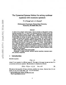
Suppose we plot the two equations x2 = w and w = 1 − y2 as graphs on a computer screen. The result for each equation, say the first one above, will be an array of pixels—some on and some off—that represents the set of ( x, w)-points which satisfy. What happens if we consider each such pixel array as a matrix of booleans—True’s and False’s—and we proceed to multiply the two matrices together? It turns out that the resulting pixel array represents the ( x, y)-pairs that simultaneously solve the two equations in the system. In other words, ordinary matrix multiplication returns a circle, x2 + y2 = 1; see Figure 1. ∗ This

project was supported by AFOSR grant FA9550-14-1-0031 and NASA grant NNH13ZEA001N-SSAT.

1

2. General approach

a.

2

c.

b.

Figure 1: Parts a and b show plots of x2 = w and w = 1 − y2 , as pixel matrices, where each entry is a 0 or 1. The pixel is black or "on" if that entry in the matrix is 1, and white or "off" if the entry is 0. The graphs appear rotated 90◦ clockwise, in order to agree with matrix-style indexing, where the first coordinate is indexed downward and the second coordinate is indexed rightward, rather than ordinary Cartesian-style indexing, where the first coordinate indexed rightward and the second coordinate indexed upward. These matrices are multiplied, and the result is shown in part c. The orange lines in parts a and b indicate an example row and column whose dot product is 1, hence a point is drawn at their intersection in part c. The fact that the result of matrix multiplication looks like a circle is not a coincidence; it is the graph of the simultaneous solution to the system given in parts a and b, which in this case can be rewritten to a single equation x2 = 1 − y2 .

This simple fact about pixel matrix multiplication MN has two counterparts, corresponding to matrix tensor product M ⊗ N and matrix trace Tr( M); and the three together form the basis of the pixel matrix approach to solving systems. The PM technique, which we will briefly discuss below, appears to be unknown, though it is easily explained. There is nothing magical in this approach; it is simply a way to organize substitution and existential quantification into a matrix arithmetic formalism. This is analogous to the sense in which Gaussian elimination simply organizes the computation necessary for solving linear systems of equations, and how matrix multiplication simply organizes the computation necessary for composing linear transformations between vector spaces with chosen bases. Matrices are quite diverse in their applications—for example they are used to study graphs, Markov processes, finite metric spaces, linear transformations, etc.—we simply add another member to the list: solving nonlinear systems.

2.2

Systems of relations, wiring diagrams, and matrices

Suppose given a system of n equations, inequalities, or other relations R1 , . . . , Rn , each of which includes some subset of k variables x1 , . . . , xk . Often, not every relation will use every variable—that is, the system is partially decomposable [Sim91]—and only some of the variables have relevant values, the rest being considered latent or internal variables [WP13]. (In Section 2.1, x and y were relevant and w was internal). For example, suppose we want to find all (v, z) pairs for which the following system of three relations R1 , R2 , R3 has a solution in a certain range (say b, v, w, x, y, z ∈ [−2, 2]): R1 :

x 2 + 3| x − y | − 5 = 0

R2 :

y2 v3 − w5 ≤ 0

R3 :

(1)

2

∃b. cos(b + zx ) − w = 0

Each of the three relations can be plotted, in some range, tolerance, and level of pixel refinement, and the result is called a pixel matrix; at the risk of confusion, we denote the corresponding boolean matrices

3. Potential advantages of the approach

3

again by R1 , R2 , R3 . One then forms an associated wiring diagram, which shows how variables are shared among the relations (e.g., y is shared by R1 and R2 ):1 S v

v x

R1

R2

w

R3

y

z x

z

(2) The wires that emerge from the outer box are v and z, as these were the relevant variables from the original query. The wiring diagram [Spi15] tells us what arithmetic operations to perform on the corresponding pixel matrices. Serial composition corresponds to matrix multiplication R1 R2 , parallel composition corresponds to matrix tensor product (forming block matrices) R1 ⊗ R2 , and feedback corresponds to partial trace Tr( R): R1 ⊗ R2 R1 R2 R1

R1 R2 R2

Tr( R) C A

R

C

(3)

B


Thus the diagram in (2) represents the formula S = Tr ( R1 ⊗ Iv ) R2 R3 , where Iv is an identity matrix. To recapitulate, we can solve system (1), we begin by plotting the three relations R1 , R2 , R3 and considering the plots as matrices of booleans, say 500 × 500. We then tensor matrix R1 by an identity matrix Iv , and multiply the result with R2 and R3 . This will produce a block matrix with square ( x × x )-blocks; taking the trace of each block will result in a matrix S of booleans, which we can plot as a 500 × 500 array of pixels. It shows the set of (v, z) pairs for which a simultaneous solution exists. Although this procedure is quite simple—involving only matrix arithmetic—it produces an approximate solution set for the fairly complex system (1).

3 3.1

Potential advantages of the approach Simplicity and support

The simplicity of the basic approach—using pixel matrix arithmetic to solve general systems—means that there is low barrier to entry for both researchers and users. There are many open questions, and mathematicians and software engineers of all stripes may be able to contribute new ideas that extend the basic seed presented here. The technique relies on matrix arithmetic and multidimensional array handling, which are the "bread and butter" of any computational software system, such as MATLAB or Julia. Programming the PM technique on top of such a numerical computing environment could be given as a final undergraduate project; for example, the current implementation involves under 500 lines of code. In other words, solving systems of relations using pixel matrices essentially "runs for free" on top of such systems. Improvements in the speed of matrix and sparse matrix arithmetic, as well as the speed of graphics processing units (GPUs) which are adept at handling the necessary sorts of vector arithmetic, will produce immediate improvements in the speed of the PM approach to solving nonlinear systems. 1 The wiring diagram is not canonically associated to the system: each box can be oriented in several ways, but all orientations give the same final result.

3. Potential advantages of the approach

3.2

4

Propagation of true negatives

As explained above, in the PM technique, one begins to solve a system of relations by plotting each one as a pixel matrix, where each pixel represents an d-dimensional rectangle. It would be best if a given pixel were to be on (true) if and only if the relation holds for some point inside the corresponding rectangle. However, even if this is true for the original plots, the results lose fidelity as the matrix operations are performed. At least in certain cases it is possible to ensure that the plot of relation R includes true negatives, i.e., that if a pixel is off (false) then no point inside the rectangle satisfies the relation. If this holds, it is a theorem that there will be no false negatives in the result of the matrix calculation for the system of relations. False positives can emerge under pixel matrix arithmetic, but as we refine the mesh the error from false positives goes down, as one would expect. The upshot is that one can get a rough estimate of the solution set by pixelating with a very coarse mesh—the result of which will be very fast—and then refine as desired inside only those pixels that are "on".

3.3

Entire solution set

When bounds for each variable are chosen, the PM approach approximates the entire solution set in the corresponding rectangle. This is in contrast to iterative nonlinear systems solvers, which generally find only one solution and require a good initial guess [QS93]. Using the mesh refinement technique from Section 3.2, one could begin by approximating the solution set using a PM technique, and then choose any "on"-pixel with which to seed a more sophisticated nonlinear systems solver.

3.4

Naturally parallelized

To solve large systems of relations, it is advantageous to paralellize the solution algorithm. The wiring diagram formalism lends itself to parallelization. Any region of the wiring diagram can be "cordoned off", and the corresponding subsystem of relations can be solved independently. Then the results can be combined to produce the correct solution set for the whole system.2 For example, below, the matrix operations needed to solve the five relations X11 , . . . , X22 can be computed by first solving the first three to form relation Y1 and the last two to form Y2 , according to the wiring subdiagrams shown here: Z Y1 X11

Y2

X13 X12

X22 X21

(4) We now have a system of two relations Y1 and Y2 , and applying a matrix multiplication and trace results in the total solution Z. The computation for Z proceeds from Y1 and Y2 without needing any information about the internal structure—nor the relations themselves—that went into computing Y1 and Y2 .

3.5

Highly tunable: solution counts, densities

As discussed above, pixel matrices have boolean entries, but these can be replaced by elements of any semiring, meaning a set S with elements 0, 1 ∈ S and operations +, × : S × S → S satisfying well-known properties. For example, using the natural numbers 0, 1, 2, . . . instead of the booleans, the PM approach will report the number of solutions, rather than just the existence of a solution. Values in the semiring R+ 2 Results

of this sort are proved category-theoretically; as an example, see [Spi15].

4. Future work of nonnegative reals would instead encode the density of solutions. Other semirings may have interesting semantics as well.

3.6

Real data, lost equations, and concept algebra

The PM technique does not require the relations or densities (see Section 3.5) to come from equations or inequalities. A scientist may have raw data relating variables x and y and more raw data relating variables y and z. A standard approach is to fit smooth functions to these data sets and to then solve the system of equations; however, curve-fitting requires a choice of model. There is often a trade-off between simplicity of the model and accuracy of fit, and any error that does arise in this way is an artifact of the choice of model, adding a confounding complication. The PM technique allows one to solve the system directly—without curve fitting—thus bypassing this minefield completely. In a similar vein, pixel matrix arithmetic works perfectly well starting with a set of related graphs as input, i.e., in cases where the equations that generated the graphs are unavailable. Similarly, the notion of concept from computational learning theory is equivalent to that of pixel matrices [KV94]. Composing concepts becomes a matter of matrix arithmetic.

4

Future work

While the basic idea is simple and can be put directly to use, there is work to be done to evaluate and improve the technique. For example, there are questions regarding algorithmic complexity and accuracy. There is also an opportunity to find innovative applications and extensions to the technique itself. Accuracy Each pixelated relation may be given an error bound, e.g., the maximum distance (say, in the L2 -metric) from a false positive to the nearest true positive. Even for a perfectly plotted relation, this will generally be nonzero because pixels have nonzero radius. One can ask: given an error bound on each relation Ri , and given a wiring diagram describing a sharing of variables between the relations, what is the error bound on the result? Another avenue would be to use probabilistic—rather than boolean—pixels to mitigate the cost of undersampling. Algorithmic complexity It is very important to understand the algorithmic complexity of the PM technique, in various cases. An important case is when the relations involved are all equations— not inequalities or arbitrary relations—in which case the pixel matrices are all sparse, reducing the complexity enormously. For example, computing x2 + y2 = 1 is much faster by using sparse matrix multiplication, as above in Section 2.1, than by using pure brute force sampling. However, for general relations the complexity appears to be exponential in the maximum, over all relations Ri , of the number of variables in Ri . Making all such bounds more precise is a high priority. Innovations There appears to be a great deal of room for finding innovative applications and extensions to the PM technique. The idea is simple enough that it can be explained easily and a prototype can be programmed quite rapidly. It follows that finding new applications areas should not be challenging. Innovations, including changes to the semiring (see Section 3.5), are similarly quite likely. Improvements in the matrix arithmetic package for boolean (bit) matrices, which could perhaps involve the lowest level machine code, could be sought. In short, there are many directions from which substantial improvements could be forthcoming.

Bibliography [AC04]

Samson Abramsky and Bob Coecke. A categorical semantics of quantum protocols. In Logic in Computer Science, 2004. Proceedings of the 19th Annual IEEE Symposium on, pages 415–425. IEEE, 2004.

5

Bibliography [Bae13]

John Baez. The foundations of applied mathematics, 2013.

[Bro65]

Charles G Broyden. A class of methods for solving nonlinear simultaneous equations. Mathematics of computation, 19(92):577–593, 1965.

[BW90]

Michael Barr and Charles Wells. Category theory for computing science, volume 49. Prentice Hall New York, 1990.

[CGR12] Justin Curry, Robert Ghrist, and Michael Robinson. Euler calculus with applications to signals and sensing. In Proceedings of Symposia in Applied Mathematics, volume 70, pages 75–146, 2012. [CKY89] John F Canny, Erich Kaltofen, and Lakshman Yagati. Solving systems of nonlinear polynomial equations faster. In Proceedings of the ACM-SIGSAM 1989 international symposium on Symbolic and algebraic computation, pages 121–128. ACM, 1989. [CW87] Don Coppersmith and Shmuel Winograd. Matrix multiplication via arithmetic progressions. In Proceedings of the nineteenth annual ACM symposium on Theory of computing, pages 1–6. ACM, 1987. [DOB15] Steven Dalton, Luke Olson, and Nathan Bell. Optimizing sparse matrixÑmatrix multiplication for the gpu. ACM Transactions on Mathematical Software (TOMS), 41(4):25, 2015. [FSH04] Kayvon Fatahalian, Jeremy Sugerman, and Pat Hanrahan. Understanding the efficiency of gpu algorithms for matrix-matrix multiplication. In Proceedings of the ACM SIGGRAPH/EUROGRAPHICS conference on Graphics hardware, pages 133–137. ACM, 2004. [GG08]

Kazushige Goto and Robert A Geijn. Anatomy of high-performance matrix multiplication. ACM Transactions on Mathematical Software (TOMS), 34(3):12, 2008.

[GSB12] Tristan Giesa, David I Spivak, and Markus J Buehler. Category theory based solution for the building block replacement problem in materials design. Advanced Engineering Materials, 14(9):810–817, 2012. [GV88]

D Yu Grigor’ev and NN Vorobjov. Solving systems of polynomial inequalities in subexponential time. Journal of symbolic computation, 5(1):37–64, 1988.

[KV94]

Michael J Kearns and Umesh Virkumar Vazirani. An introduction to computational learning theory. MIT press, 1994.

[Mar00] José Mario Martınez. Practical quasi-newton methods for solving nonlinear systems. Journal of Computational and Applied Mathematics, 124(1):97–121, 2000. [QS93]

Liqun Qi and Jie Sun. A nonsmooth version of newton’s method. Mathematical programming, 58(1-3):353–367, 1993.

[Sim91] Herbert A Simon. The architecture of complexity. Springer, 1991. [Spi14]

David I Spivak. Category theory for the sciences. MIT Press, 2014.

[Spi15]

David I Spivak. The steady states of coupled dynamical systems compose according to matrix arithmetic. arXiv preprint arXiv:1512.00802, 2015.

[Stu02]

Bernd Sturmfels. Solving systems of polynomial equations. Number 97. American Mathematical Soc., 2002.

[WP13]

Jan C Willems and Jan W Polderman. Introduction to mathematical systems theory: a behavioral approach, volume 26. Springer Science & Business Media, 2013.

6