Summary. Both island-biogeographic (dynamic) and niche-based (static) metapopulation models make predictions about the distribution and abundance of ...
Evolutionary Ecology 1997, 11, 275±288
Placing empirical limits on metapopulation models for terrestrial plants S A M U E L M . S C H E I N E R 1 * a n d J O S EÂ M . R E Y - B E N A Y A S 2 1 2
Department of Life Sciences (2352), Arizona State University West, PO Box 37100, Phoenix, AZ 85069, USA Area de EcologõÂa, Facultad de Ciencias, Universidad de AlcalaÂ, E-28871 Alcala de Henares, Madrid, Spain
Summary Both island-biogeographic (dynamic) and niche-based (static) metapopulation models make predictions about the distribution and abundance of species assemblages. We tested the utility of these models concerning such predictions for terrestrial vascular plants using data from 74 landscapes across the globe. We examined correlations between species frequency and local abundance and shapes of the species frequency distribution. No data set met all of the predictions of any single island-biogeographic metapopulation model. In contrast, all data sets met the predictions of the niche-based model. We conclude that in predicting the distribution of species assemblages of plants over scales greater than 10±1 km, niche-based models are robust while current metapopulation models are insucient. We discuss limitations in the assumptions of the various models and the types of empirical observations that they will each have to deal with in further developments. Keywords: island biogeography, niche-based models; species distributions; terrestrial plants
Introduction Explaining the distribution and abundance of species has been a central question in ecology since its inception. Attacks on this problem come from two directions: (1) starting with empirical data and looking for regularities or correlations with putative causal factors and (2) starting with theoretical considerations and looking for con®rming patterns (Levin, 1992). Currently, despite a century of eorts, ecologists have no clear consensus based on results from either approach. Necessary to this enterprise is the critical testing of theoretical approaches against empirical data, especially those that have widespread support. We examined two classes of models of species distributions. The ®rst class is dynamic and arose out of island-biogeography theory (MacArthur and Wilson, 1967). This theory explains the distribution of species among islands or island-like habitats (e.g. mountain tops, forest patches) as a balance between the processes of colonization (immigration) and local extinction. Based on these ideas, Levins (1969; Gilpin and Hanski, 1991) conceived the metapopulation, an archipelago of semi-isolated populations linked by processes of immigration and emigration. Two critical assumptions of these models are: (1) that the environment is relatively homogeneous across populations and (2) that metapopulations are suciently subdivided that populations can ¯uctuate and go extinct independently yet still be connected by immigration, although these assumptions can be relaxed (e.g. Hanski and Gyllenberg, 1993; Hastings and Harrison, 1994). This class of models has been extensively developed in the past decade (Gilpin and Hanski, 1991; Hastings and Harrison, 1994). A third critical assumption is necessary to use these models to make predictions about species assemblages: the migration and extinction patterns of any group of species ± species' *
Author to whom all correspondence should be addressed.
0269-7653
Ó 1997 Chapman & Hall
276
Scheiner and Rey-Benayas
reactions to the environment ± are similar. Some evidence for the validity of metapopulation models exists for animals (Gilpin and Hanski, 1991), although others dispute this claim (Gaston and Lawton, 1989; Tokeshi, 1992; Hastings and Harrison, 1994). The models developed within this framework have the general form: dp=dt immigration rate ÿ extinction rate
1
where p is the percentage of occupied sites of a given species, 0 £ p £ 1 (Gotelli, 1995). If both the immigration rate and the extinction rate are a function of p, the model takes the form (Hanski, 1982): dp=dt ip
1 ÿ p ÿ ep
1 ÿ p
2
That is, immigration rate is a function of the probability of immigration, i, times the fraction of available sources for colonists, p, times the fraction of available sites, 1 ) p. Extinction rate is a function of the probability of extinction, e, times the fraction of sites with populations that can go extinct, p, times one minus the fraction of sites that can provide emigrants thereby reducing the probability of local extinction, 1 ) p, the `rescue eect'. If both processes are independent of occupancy, the model reduces to (Gotelli, 1991): dp=dt i
1 ÿ p ÿ ep
3
Gotelli (1991) refers to occupancy-independent immigration as the `propagule rain'. All four possible combinations of occupancy-dependent and occupancy-independent immigration rate and extinction rate are conceivable (see Table 1; Gotelli, 1991). These models represent the extremes of a more general metapopulation model (Gotelli and Kelley, 1993). The occupancy eect is referred to as a density eect in many papers (e.g. Hanski, 1982; Gotelli, 1991), but Gotelli (1995) points out that such usage can confuse within-population processes with between-population processes. The various versions of this model make explicit predictions about two aspects of species distributions (Table 1): 1. If local extinction rates are dependent on population occupancies, then those species in a landscape with a high frequency ± occurring in a large number of sites ± will also have a high mean abundance when present in a site, a positive correlation between frequency and abundance. If the process is occupancy-independent, the correlation will be zero. According to
Table 1. Models of species distribution and abundance and their predictions regarding the correlation between species frequency and abundance and the shape of the frequency distribution. Metapopulation models are classi®ed by the dependence of immigration and extinction rates on the percentage of occupied sites Eect Model
Immigration
Predictions Extinction
Correlation
Distribution
Reference
Island-biogeographic metapopulation models 1 Dependent Dependent 2 Dependent Independent 3 Independent Dependent 4 Independent Independent
Positive Zero Positive Zero
Bimodal Single interior mode Single interior mode Single interior mode
Hanski (1982) Levins (1969) Gotelli (1991) Gotelli (1991)
Niche-based models 5 None
Positive
Single mode at 1
Brown (1984)
None
Testing metapopulation models
277
Tokeshi (1992), this positive correlation is an assumption of the models rather than a prediction. We note that for present purposes of examining the empirical scope of these models, this distinction does not matter. We will examine data for this correlation. If the correlations are positive, for example, we can state that the occupancy-independent models do not ®t the data, whether one considers this lack of ®t to be a failure of assumptions or a failure of predictions. 2. If both immigration and extinction rates are occupancy-dependent, then species frequencies will have a bimodal distribution (Fig. 1A). Species will tend to be either very common or very rare, although they may switch over time. That is, commonness is not a permanent property of a species. This aspect of this model is referred to as the `core-satellite hypothesis' (Hanski, 1982; Hanski and Gyllenberg, 1993). If either rate is occupancy-independent, the distribution will be unimodal with the mode located somewhere in the middle of the distribution (Fig. 1B). That is, the most typical species will be somewhat common, with exact values depending on immigration and extinction rates (Gotelli, 1991; Tokeshi, 1992). We will inspect our data for conformity to these various distributions. The other class of models is static and based on local ecological sorting processes; they are referred to as niche-based models (Brown, 1984, 1995; Collins and Glenn, 1991) or ecological specialization models (Hanski et al., 1993). These models assume that all species can potentially disperse throughout the landscape and that variation in species tolerances to continuously varying local conditions ± the abiotic environment and biotic interactions such as competition and predation ± determine species distributions. In its most explicit form, distributions of abundances are assumed to be roughly Gaussian (or at least unimodal) across environmental gradients, leading to two predictions (Brown, 1984): (1) species frequencies and abundances will be positively correlated; (2) frequency distributions will be unimodal with the mode at or near one (Fig. 1C). That is, widespread species are able to exploit a wide range of resources and become locally abundant (Gaston and Lawton, 1990), while the typical species in a given landscape will be found in few or a single location. Alternatively, the positive correlation could be due to dierences in the distribution of resources used by dierent species. Beyond the predictions shared with the island-biogeographic models, Brown (1984) makes an additional prediction that an increase in the number of underlying environmental gradients would coincide with a more J-shaped species frequency distribution (i.e. a stronger mode at one), because with more gradients specialists are restricted to a smaller and smaller portion of the entire region.
Figure 1. Species frequency distributions predicted by various theories. (A) Metapopulation models that assume that immigration rates and emigration rates are occupancy-dependent. (B) Metapopulation models that assume that either immigration rates or emigration rates are occupancy-independent. (C) Niche-based models (after Collins and Glenn, 1991).
278
Scheiner and Rey-Benayas
The two classes of models, although accounting for the same ecological properties and not explicitly scale-dependent, may be relevant at very dierent scales (Collins and Glenn, 1991; Levin, 1992). Island-biogeographic models are potentially most appropriate at small scales where processes of colonization and extinction will predominate (101 km or less among patches). Nichebased models are potentially most appropriate at large scales where environmental heterogeneity and ecological sorting processes will predominate (103 km or more among patches). We do not know the upper or lower limits of applicability of these models and the relevancy of dierent models for dierent types of habitats. Clearly, the appropriate limits on these processes will vary for any group of organisms depending on typical dispersal rates and distances and on perceived environmental heterogeneity. The values given here are those most likely to be appropriate for terrestrial plants. Our examination of metapopulation models is appropriate because they have been, and continue to be, applied to terrestrial plant landscapes (e.g. Gotelli and Simberlo, 1987; Collins and Glenn, 1990; Hanski et al., 1993). One potential criticism of our approach is the use of multispecies data with a theory developed in the context of single-species dynamics. We defend our approach in two ways. First, those who developed these theories claim suitability in this context (e.g. Hanski et al., 1993). As currently used, these theories predict either the frequency distribution of a single species over time or the distribution of an array of species at a single time over space. Second, while it is true that species are not ecologically identical, the test of the theory does not require them to be so. The predictions regarding species frequencies (row totals in a site±species data matrix) are independent of community richness (column totals). Ecological equivalence will aect the latter, not the former. For example, rare species might all be concentrated in a single community, or they might be randomly distributed among all sites. Which is the case will depend on the ecological equivalence among species. However, either pattern would result in exactly the same species frequency distribution. Variation among species might obscure frequency distribution patterns if small dierences in niches, immigration rates and extinction rates spread out peaks in the distribution. In particular, bimodal distributions will be most aected. However, the patterns we found (see below) deviate so strongly from the predictions that metapopulation dynamics appear unable to explain any of the distributions. Multispecies data are inappropriately applied to such models if immigration and extinction rates are so species-speci®c that no assemblage-wide predictions are possible. But we question whether these rates are even constant for a given species, leaving the utility of the entire theory in question. We wish to make clear that we are not addressing the correctness of these various models. Unless there is an error in the mathematics, a theoretical model can never be `wrong'. Rather, the issue is the pertinence of a given model to a particular empirical realm. Materials and methods We address the issue of model relevance by testing their assumptions and predictions for terrestrial vascular plants distributed among sites in landscapes. The data consisted of surveys of 74 terrestrial landscapes from across the globe (see Appendix). The total latitudinal range was 43°S to 81°N with 36 tropical or subtropical (0° to 35°), 31 temperate (36° to 55°) and 5 polar (64° to 81°) landscapes. The landscapes came from all continents except Antarctica: North America (n = 23), South America (n = 1), Eurasia (n = 22), Africa (n = 17), Australia (n = 15). The landscapes included a wide variety of habitats: tropical forests (n = 10), tropical grasslands (n = 7), shrublands (n = 7), deserts (n = 7), wetlands (n = 3), temperate grasslands (n = 3), temperate broadleaved forests (n = 14), temperate needle-leaved forests (n = 4), boreal forests (n = 4), tundras (n = 14). Landscape extent surveyed ranged from 0.5 to 740,000 km2 (mean 755 km2 = a circle of radius 15.5 km). Surveys were restricted to only those for which one type of habitat was sampled (e.g. just forests
Testing metapopulation models
279
within a forest±grassland mosaic). The mean number of sites sampled within each landscape was 67.5 (range 20±137). Site sizes ranged from 0.5 m2 for high arctic landscapes to 10 ha for tropical landscapes (mean 1.6 ha). More information, including a map showing landscape locations and a complete list of data sources, is given in Scheiner and Rey-Benayas (1994). Copies of most of the data sets are available from S.M. Scheiner upon request. Each of the models makes a series of predictions about species distributions in landscapes, and the totality of those predictions are mutually exclusive (Table 1). We examined each of the 74 data sets for conformity to those predictions looking for consistency with any one model. For these analyses, the frequency of each species was measured as the number of sites in which that species appeared. The abundance of each species was measured as the mean density of that species across all sites for which it was at least present (density greater than zero). For the 74 surveys, dierent authors used dierent survey methods or measured abundance in dierent ways. But our analyses of correlations or examinations of frequency distributions are not biased, as each analysis was done within a single, self-consistent data set. These data provide a strong test of the empirical scope of the models because of their global extent and wide representation of habitat types. The range in scales of these landscapes (0.5 ± 740,000 km2) allows for the imposition of clear scale constraints of the applicability of these models. Results First, we test predictions concerning the correlation between landscape frequency (number of sites occupied) and local abundance (mean density in occupied sites). The data used came only from those surveys that included measures of absolute abundance (see Appendix). The 15 suitable data sets included three tropical grasslands, four temperate forests, one temperate shrubland, one prairie, three boreal forests and three tundras. All of the correlations were positive with a median value of 0.47 (Fig. 2). Such a correlation could be due to sampling artefacts (Wright, 1991). If individuals are distributed by a Poisson process, then a regression of the logarithm of absences (ln(1)p)) against abundance will have a slope of 1.0 and an intercept of 0.0. For our data sets, the slopes ranged from 0.0 to )0.05 and the intercepts ranged from )0.9 to 0.2. In only two instances were the intercepts not statistically dierent from 0. Sampling artefacts are, therefore, an unlikely source of the positive correlations (see also Wright, 1991). Thus we deem unsuitable for this range of spatial scales those metapopulation models with occupancy-independent extinction rates, as they predict a zero correlation (Models 2 and 4, Table 1). Next we test predictions concerning the distribution of species frequencies. Four representative examples are shown in Fig. 3. We examined the shapes of the distributions for the 74 data sets both statistically and visually. Although a general test for bimodality does not exist (Ellison, 1993), there is a test for unimodality ± the dip test (Hartigan, 1985; Hartigan and Hartigan, 1985). All but nine of the data sets were signi®cantly unimodal (P < 0.01). All data sets, but especially those that were not unimodal, were also examined visually using stem-leaf plots and tables of species frequencies generated with SYSTAT (Wilkinson, 1988; Ellison, 1993). Of the nine non-statistically unimodal data sets, seven consisted of either a uniform distribution or a distribution with a small mode at or near 1 (i.e. p » 0) and a very long tail (e.g. Fig. 3A). Five of these landscapes were tundras or a northern wetland. The other two non-statistically unimodal data sets each had a shoulder near the mode (e.g. Fig. 3C). We also looked speci®cally for evidence of bimodality as predicted by the island-biogeographic models (Fig. 1A). Bimodality was assessed by looking for species with frequencies equal to the maximum possible, the total number of sites. Only four landscapes had such species. For three landscapes, these consisted of a single species. The fourth landscape was an arctic tundra with a ¯at frequency distribution (Fig. 3A). None of the distributions were bimodal in the sense predicted by the theory (modes at 1 and the maximum number of sites). Nor was there any
280
Scheiner and Rey-Benayas
Figure 2. Frequency distribution of Spearman rank correlations of species frequencies and local abundance for 15 landscapes (median = 0.47, range = 0.11±0.74). All values except the smallest (shaded portion) are signi®cantly dierent from 0 ( P < 0.005). Similar results were obtained using a Pearson product±moment correlation and log10(abundance) (median = 0.41, range = 0.01±0.64; 13 values signi®cantly dierent from 0, P < 0.01). All statistical analyses were done with SYSTAT (Wilkinson, 1988).
indication, for any landscape, of a mode at the maximum number of sites occupied even if that was less than the total possible number of sites. Thus we deem unsuitable for this range of spatial scales those metapopulation models with occupancy-dependent extinction and immigration rates as they predict bimodal distributions (Model 1, Table 1). With further examination, we found that the modes of the distributions were almost always 1 or 2 (i.e. p » 0) (Table 2). For those landscapes with modes of 3, 4 or 6, we make the following further observations: (1) these modes are still very close to 1 relative to the possible maxima; (2) we found no apparent pattern among these landscapes. They include four tropical forests, one temperate forest, one warm desert, one alpine tundra and one arctic tundra. Other similar landscapes had modes of 1 or 2. We conclude that landscapes with modes greater than 2 most likely resulted from random variation or from a failure to intensively survey for rare species, especially in rich tropical communities. Although we only used data sets which included rare species, intensity of sampling will aect the observed frequency of rare species. Thus we deem unsuitable for this range of spatial scales those metapopulation models with either immigration or extinction rates that are occupancy-independent, as they predict that the typical species will be somewhat common (Models 2±4, Table 1). Regarding the niche-based model prediction of the number of environmental gradients and the shape of the species frequency distribution, we quanti®ed this relationship using two measures. A ¯at vs J-shaped distribution was quanti®ed as the standard deviation of species frequencies (i.e. the variation in the heights of the bars in the species frequency diagram; Fig. 3). A more J-shaped distribution would have a greater standard deviation. The number of underlying gradients was measured as mosaic diversity (Scheiner, 1992) with a higher value of mosaic diversity indicating
Testing metapopulation models
281
Figure 3. Species frequency distributions of four representative landscapes. For all graphs, the abcissa is scaled to the total number of sites sampled. (A) Arctic tundra, Devon Island, Canada (Muc, 1976); (B) evergreen broadleaf forest, Italy (Gerdol et al., 1985); (C) evergreen broadleaf forest, South Africa (Campbell and Moll, 1977); (D) tropical rainforest, Ghana (Hall and Swaine, 1981).
more gradients. Mathematically mosaic diversity is a function of the variation in species richness among communities and the variation in commonness or rarity among species. These two measures are strongly positively correlated for our landscapes (r = 0.61, P < 0.0001; Fig. 4), indicating that a more J-shaped distribution is associated with a greater number of underlying environmental
Table 2. Modes of species frequency distribution from 74 landscapes of terrestrial vascular plants (Scheiner and Rey-Benayas, 1994). Most landscapes have modes of 1 or 2 (i.e. p » 0). Numbers sum to 75 because one landscape (Fig. 3B) had modes at both 2 and 6 Mode Number of landscapes
1 54
1.5 2
2 11
3 2
4 4
5 0
6 2
282
Scheiner and Rey-Benayas
Figure 4. The relationship between the number of underlying gradients ± measured as mosaic diversity ± and the extent to which the species frequency distribution is ¯at or J-shaped ± measured as the standard deviation of species frequencies for 74 terrestrial plant landscapes.
gradients. Such a correlation could be due to sampling artefacts if increasing the number of quadrats sampled simultaneously resulted in a greater value for mosaic diversity and increased the number of rare species found. A multiple regression analysis of the standard deviation in species frequency against mosaic diversity and the number of quadrats sampled found no such sampling eect (b¢ = )0.13, P = 0.19). Discussion None of the island-biogeographic models was able to correctly predict the distribution of terrestrial vascular plants across landscapes at scales of about 10)1 to 106 km2. While some predictions held for some models, all failed at least one prediction. For example, the single landscape (an African grassland) that had a non-signi®cant ± albeit positive ± correlation of species frequency and abundance had a mode of 1 for the species frequency distribution. Only the niche-based model successfully predicted those distributions (Model 5, Table 1). It predicts (1) a positive correlation of frequency and abundance, (2) frequency distributions will be unimodal with the mode at or near 1, and (3) a positive correlation between the number of environmental gradients and a more J-shaped species frequency distribution. Our results cannot be construed to indicate that the niche-based model is the correct explanation for terrestrial plant species distributions. Rather, it is the only model presently developed that is fully consistent with the current evidence for terrestrial plants at scales greater than 1 km2. The general consistency of our results, despite the wide variety of data sources, argues for the robustness of our conclusions. We were actually quite surprised at the consistency among landscapes, fully expecting dierences based on either habitat type or latitude. Based on the distribution of modal values, one can argue that metapopulation models with occupancy-dependent extinction rates and occupancy-independent immigration rates (Model 3, Table 1) are possibly consistent
Testing metapopulation models
283
with our results. However, such a metapopulation model would require very low immigration rates and moderate to high extinction rates (Gotelli, 1991). These extinction rates are very unlikely for perennial plant communities, especially those with trees. A model with occupancy-dependent extinction and immigration rates does not necessarily result in a bimodal distribution; if background extinction rates are greater than 0, a single interior mode is predicted (Gotelli and Kelley, 1993). However, this prediction is still inconsistent with our data. Thus none of these metapopulation models can be reasonably stretched to ®t these data. Other data for terrestrial plant communities are also consistent with our conclusions. Nearly all investigators have found positive correlations between species frequency and abundance at all spatial scales (Hanski, 1982; Brown, 1984, 1995; Gotelli and Simberlo, 1987; Collins and Glenn, 1991; Hanski and Gyllenberg, 1993), although some have not (Wright, 1991). Species frequency distributions usually have a single mode at or near 1 (Brown, 1984, 1995). One series of studies of tallgrass prairie communities (Gotelli and Simberlo, 1987; Collins and Glenn, 1990, 1991) seems to show evidence of bimodal distributions for surveys done at a scale of 1 km2 or less. These are the only data to show any evidence of bimodality and they are on a scale much smaller than ours or other data sets. Claims about bimodal distributions have been challenged generally as being either a sampling artefact or a function of variation in carrying capacities among sites (Nee et al., 1991), although this has been disputed (Hanski, 1991). Thus at medium to large scales, no single study of any terrestrial plant landscape, either ours or others, is consistent with all predictions of any single island-biogeographic metapopulation model. One could argue that metapopulation models should not be judged against our data because of a failure to meet the assumptions of the models. However, this objection misses the purpose of our project. We are not judging the correctness of the models. Assuming that the mathematics was done properly, any model is correct. The empirical scope of that model is a separate issue, however. Metapopulation models may still be appropriate for predicting the distributions of single species or multispecies assemblages at small spatial scales. Our goal in this paper was to see if the metapopulation models made accurate predictions for multispecies terrestrial plant systems and, if they failed to do so, to provide some explanation for their failure. One could argue that particular data sets do not even approach the assumptions of the islandbiogeographic metapopulation models. We certainly cannot defend the use of all 74 data sets within the scope of this paper. Given the consistency of our results, however, one would need to reject all of our data sets to invalidate our conclusions. A complete listing of sources is available in Scheiner and Rey-Benayas (1994) so that readers can judge for themselves the appropriateness of our data. Tokeshi (1992) presented a variant on the island-biogeographic models in which the extinction rate is a decreasing function of species frequency: dp=dt ip
1 ÿ p ÿ e
1 ÿ p
4
Tokeshi bases this model on the following reasoning. More widespread species tend to have a higher local abundance, with a positive correlation between frequency and abundance. Abundant species should have a lower extinction rate than rare species. The result is a negative correlation of species frequency and extinction rate. Empirical evidence supports this claim (Simberlo and Wilson, 1970; Diamond, 1984; Schoener and Spiller, 1992). This model is consistent with our data. It assumes a positive correlation between frequency and abundance and predicts that species frequency distributions will either be ¯at or have a mode at or near 1, depending on immigration and extinction probabilities. However, this model has a logical ¯aw. The extinction probability, e, is just that, a probability. We ®nd it illogical that one would not multiply that probability by the fraction of populations occupied, p, to obtain an extinction rate.
284
Scheiner and Rey-Benayas
Tokeshi (1992) is correct that other metapopulation models are inconsistent with the evidence regarding extinction rates. If we take as given that frequency and abundance are positively correlated, then the models assume either a quadratic relationship between abundance and extinction (Equation 2), or a positive relationship (Equation 3) rather than a negative relationship. On the other hand, a general metapopulation model can be made consistent with a negative correlation between frequency and extinction rate (Gotelli and Kelley, 1993). What is not yet clear is whether this more general model can result in species frequency distributions that are consistent with the data presented here using realistic values for immigration and extinction rates. We conclude that current island-biogeographic metapopulation models do not account for the distribution of multispecies assemblages of terrestrial vascular plants. Our results put an upper limit to the applicability of these models at scales of approximately 1 km2 or less, and no other study of terrestrial plants has been shown to be completely consistent with these models. Our results add to the growing body of evidence (see review in Hastings and Harrison, 1994) that the widely used versions of metapopulation models examined here do not adequately describe species assemblage distributions. The likely cause for the inapplicability of these models may be due to a failure of any of the three critical assumptions listed in the Introduction: (1) environmental homogeneity, (2) the level of connectedness and (3) equality of species migration and extinction rates. We deal with each in turn. First, we ®nd unlikely the assumption of environmental homogeneity among sites. Even at very small scales (1±10 m2), the environment is heterogeneous for terrestrial plants. Hanski and Gyllenberg (1993) relax the homogeneity assumption but still predict bimodal species distributions, a distribution that we failed to ®nd in any of our data sets. Second, Hastings and Harrison (1994) ®nd little support for the connectedness assumptions made by the types of metapopulation models examined here. Instead, they propose a more general class of models that encompass more realistic migration and extinction patterns. Yet to be determined is the consistency of this more general class of models and the data presented here. For example, immigration must have a substantial eect on local population dynamics to generate a positive correlation of frequency and abundance (Hastings, 1991). Thus immigration rates for plants on a landscape scale need to be determined. Third, we ®nd more likely the assumption of equality of species migration and extinction rates ± necessary if we wish to use multispecies data to test these theories. Many of our data sets consist of only a single lifeform (e.g. just trees) or a small class of lifeforms. Our results did not depend on lifeform homogeneity within a given data set, as all types of data sets gave consistent results. Thus metapopulation models need to be developed further to make them consistent with the empirical evidence (e.g. Tokeshi, 1992; Gotelli and Kelley, 1993). Our failure to ®nd support for any of the island-biogeographic models does not provide an automatic endorsement for the alternative niche-based model. We must also deal directly with the assumptions and predictions of that model. Regarding the positive frequency±abundance correlation, Hanski et al. (1993) provide two alternative mechanisms within the niche-based model framework: (1) generalist species are both more abundant and more widespread than specialist species; (2) resources used by dierent species vary such that more widespread resources are associated with a greater local abundance of the species exploiting those resources. The second mechanism simply moves the explanation down one trophic level and, thus, is not general. Regarding the ®rst mechanism, Hanski et al. (1993) found little evidence that generalist species were either more widespread or had a higher local abundance than specialist species. But this test of the ®rst mechanism fails to address directly the model proposed by Brown (1984). One needs to disentangle species characteristics as they appear across their entire range and how they may appear within a single landscape. In Brown's concept, a species has a centre of distribution. At that centre the species is both abundant and widespread. Moving away from that centre, the species becomes progressively less abundant as habitat quality for that species decreases.
Testing metapopulation models
285
This decrease in quality also restricts the species to a smaller number of habitats. So, habitat speci®city and, especially, abundance are not necessarily general species characteristics. We would not expect a species-wide characterization of generalist or specialist to necessarily predict abundance patterns within a small part of the species' range. For example, in a survey of the British ¯ora, Rabinowitz et al. (1986) found that 149 of 160 (93%) species had large population sizes somewhere within their range whether or not the species was considered a habitat generalist or specialist. We found a consistency between global patterns in species frequency distributions and nichebased models. Species frequency distributions were relatively ¯at for high-latitude landscapes (e.g. Fig. 3A), whereas they became progressively more J-shaped (i.e. more species found in a single location with fewer widespread species) at middle and low latitudes (e.g. Figs 3C,D). This progression is re¯ected in a global gradient in mean similarity ± b diversity ± among landscapes (Scheiner and Rey-Benayas, 1994). Along a latitudinal gradient, mean similarities change in a quadratic fashion, being high (small dierences among sites) at high latitudes, reaching a minimum at 30° latitude, and then increasing again. We attributed this pattern to a global gradient in the importance of biotic interactions in structuring landscapes and high levels of competition for water in arid landscapes at 30° latitude. Our results suggest that for terrestrial vascular plants, competitive interactions as much as abiotic limitations are responsible for landscape structuring and global gradients in landscape parameters. These data must be taken into account in any further development of niche-based models. Acknowledgements We thank the many generous people who freely supplied their data for our analyses, together with B. Danielson, D. Goldberg, P. Meserve, C. Thomas, M. VanderMeulen, M. Williamson and a number of anonymous reviewers for comments on previous drafts of the manuscript. We especially thank N. Gotelli for his insightful review and suggestions for tests of sampling artefacts. Support was provided by a Fulbright Postdoctoral Fellowship to J.M.R.-B. References Brown, J.H. (1984) On the relationship between abundance and distribution of species. Am. Nat. 124, 255± 279. Brown, J.H. (1995) Macroecology. University of Chicago Press, Chicago, IL. Campbell, B.M. and Moll, E.J. (1977) The forest communities of Table Mountain, South Africa. Vegetatio 34, 105±115. Collins, S.L. and Glenn, S.M. (1990) A hierarchical analysis of species' abundance patterns in grassland vegetation. Am. Nat. 135, 633±648. Collins, S.L. and Glenn, S.M. (1991) Importance of spatial and temporal dynamics in species regional abundance and distribution. Ecology 72, 654±664. Diamond, J.M. (1984) `Normal' extinctions of isolated populations. In Extinctions (M.H. Nitecki, ed.), pp. 191±246. University of Chicago Press, Chicago, IL. Ellison, A.M. (1993) Exploratory data analysis and graphic display. In Design and Analysis of Ecological Experiments (S.M. Scheiner and J. Gurevitch, eds), pp. 14±45. Chapman and Hall, New York. Gaston, K.J. and Lawton, J.H. (1989) Insect herbivores on bracken do not support the core-satellite hypothesis. Am. Nat. 134, 761±777. Gaston, K.J. and Lawton, J.H. (1990) Eects of scale and habitat on the relationship between regional distribution and local abundance. Oikos 58, 329±335. Gerdol, R., Ferrari, C. and Piccoli, F. (1985) Correlation between soil characteristics and forest types: A study in multiple discriminant analysis. Vegetatio 60, 49±56.
286
Scheiner and Rey-Benayas
Gilpin, M. and Hanski, I. (eds) (1991) Metapopulation Dynamics: Empirical and Theoretical Investigations. Academic Press, London. Gotelli, N.J. (1991) Metapopulation models: The rescue eect, the propagule rain, and the core-satellite hypothesis. Am. Nat. 138, 768±776. Gotelli, N.J. (1995) A Primer of Ecology. Sinauer Associates, Sunderland, MA. Gotelli, N.J. and Kelley, W.G. (1993) A general model of metapopulation dynamics. Oikos 68, 36±44. Gotelli, N.J. and Simberlo, D. (1987) The distribution and abundance of tallgrass prairie plants: A test of the core-satellite hypothesis. Am. Nat. 130, 18±35. Hall, J.B. and Swaine, M.D. (1981) Distribution and Ecology of Vascular Plants in a Tropical Rainforest: Forest Vegetation in Ghana. Junk, The Hague. Hanski, I. (1982) Dynamics of regional distribution: The core and satellite hypothesis. Oikos 38, 210±221. Hanski, I. (1991) Reply to Nee, Gregory and May. Oikos 62, 88±89. Hanski, I. and Gyllenberg, M. (1993) Two general metapopulation models and the core-satellite species hypothesis. Am. Nat. 142, 17±41. Hanski, I., Kouki, J. and Halkka, A. (1993) Three explanations of the positive relationship between distribution and abundance of species. In Species Diversity in Ecological Communities (R.E. Ricklefs and D. Schluter, eds), pp. 108±116. University of Chicago Press, Chicago, IL. Hartigan, J.A. and Hartigan, P.M. (1985) The dip test of unimodality. Ann. Stat. 13, 70±84. Hartigan, P.M. (1985) Computation of the dip statistic to test for unimodality. Appl. Stat. 34, 320±325. Hastings, A. (1991) Structured models of metapopulation dynamics. Biol. J. Linn. Soc. 42, 57±71. Hastings, A. and Harrison, S. (1994) Metapopulation dynamics and genetics. Ann. Rev. Ecol. Syst. 25, 167± 188. Levin, S.A. (1992) The problem of pattern and scale in ecology. Ecology 73, 1943±1967. Levins, R. (1969) Some demographic and genetic consequences of environmental heterogeneity for biological control. Bull. Entomol. Soc. Am. 15, 237±240. MacArthur, R.H. and Wilson, E.O. (1967) The Theory of Island Biogeography. Princeton University Press, Princeton, NJ. Muc, M. (1976) Ecology and primary production of high arctic sedge-moss meadows, Devon Island, NWT, Canada. PhD dissertation, University of Edmonton, Alberta. Nee, S., Gregory, R.D. and May, R.M. (1991) Core satellite species: Theory and artefacts. Oikos 62, 83±87. Rabinowitz, D., Cairns, S. and Dillon, T. (1986) Seven forms of rarity and their frequency in the ¯ora of the British Isles. In Conservation Biology: The Science of Scarcity and Diversity (M.E. SouleÂ, ed.), pp. 182±205. Sinauer Associates, Sunderland, MA. Scheiner, S.M. (1992) Measuring pattern diversity. Ecology 73, 1860±1867. Scheiner, S.M. and Rey-Benayas, J.M. (1994) Global plant diversity: Patterns and processes. Evol. Ecol. 8, 331±347. Schoener, T.W. and Spiller, D.A. (1992) Is extinction rate related to temporal variability in population size? An empirical answer for orb spiders. Am. Nat. 139, 1176±1207. Simberlo, D.S. and Wilson, E.O. (1970) Experimental zoogeography of islands: A two-year record of colonization. Ecology 51, 934±937. Tokeshi, M. (1992) Dynamics of distribution in animal communities: Theory and analysis. Res. Pop. Ecol. 34, 249±273. Wilkinson, L. (1988) SYSTAT: The System for Statistics. SYSTAT, Evanston, IL. Wright, D.H. (1991) Correlations between incidence and abundance are expected by chance. J. Biogeogr. 18, 463±466.
Testing metapopulation models
287
Appendix The landscapes analysed, sorted by continent and biome type, indicating vegetation type, data set size and type of data (P = presence/absence, R = ranked abundance, A = absolute abundance)
Biome type
Number of sites
Number of species
Data type
Africa Savanna Savanna Savanna Savanna Savanna Shrubland Shrubland Temperate evergreen broadleaf forest Temperate rainforest Tropical rainforest Tropical rainforest Warm desert Warm desert Warm desert Warm desert Warm desert Warm desert
80 120 120 65 42 101 78 105 42 85 70 76 72 44 74 45 75
210 221 226 202 416 729 215 118 188 567 595 152 125 126 191 173 66
A P P A R R R R A P P R P P R R R
Asia Alpine boreal forest Alpine grassland Alpine tundra Alpine tundra Alpine tundra Arctic tundra Deciduous forest Shrubland Tropical rainforest Tropical seasonal forest Wetland Wetland
90 39 66 39 40 57 110 37 33 37 91 20
97 119 161 168 78 20 256 126 166 309 112 68
A R R R R R P R R P R R
Australia Savanna Shrubland Shrubland Temperate evergreen broadleaf forest Temperate rainforest Tropical rainforest Tropical rainforest Tropical rainforest Tropical rainforest Tropical rainforest Woodland
67 31 64 81 66 83 137 136 82 64 30
315 347 558 144 163 510 525 516 662 553 92
A P P R P P P P P P P
288
Scheiner and Rey-Benayas
Appendix (Cont.) Biome type
Number of sites
Number of species
Data type
Europe Alpine tundra Alpine tundra Alpine tundra Arctic tundra Grassland Shrubland Temperate evergreen broadleaf forest Temperate evergreen broadleaf forest Temperate evergreen broadleaf forest Wetland
46 32 61 68 61 128 112 40 106 37
221 131 114 76 226 130 242 64 233 28
R R R A R R R R R R
North America Alpine boreal forest Alpine boreal forest Alpine boreal forest Alpine coniferous forest Alpine coniferous forest Alpine coniferous forest Alpine tundra Alpine tundra Alpine tundra Arctic tundra Arctic tundra Arctic tundra Coniferous forest Deciduous forest Deciduous forest Deciduous forest Mixed forest Mixed forest Mixed forest Shrubland Shortgrass prairie Warm desert Wetland
40 62 21 101 129 93 56 113 20 51 20 80 56 35 33 78 119 30 88 62 32 109 42
76 99 127 426 452 442 177 261 112 85 34 69 188 266 235 556 454 222 117 61 184 100 119
R R A R R R R R R A A R A P P P P A A A A P R
41
84
R
South America Grassland