Given an ordered list of vertices L = v1,...,vn, the index of a vertex is its position in the list (i.e. vi has ...... Springer, 2005. [28] Hans L. Bodlaender and Ton Kloks.
Planar Graphs and Partial k-Trees by Philip Thomas Henderson A thesis presented to the University of Waterloo in fulfilment of the thesis requirement for the degree of Master of Mathematics in Computer Science Waterloo, Ontario, Canada, 2005 c Philip T. Henderson 2005
I hereby declare that I am the sole author of this thesis. I authorize the University of Waterloo to lend this thesis to other institutions or individuals for the purpose of scholarly research.
I further authorize the University of Waterloo to reproduce this thesis by photocopying or by other means, in total or in part, at the request of other institutions or individuals for the purpose of scholarly research.
ii
Abstract It is well-known that many N P-hard problems can be solved efficiently on graphs of bounded treewidth. We begin by showing that Knuth’s results on nested satisfiability are easily derived from this fact since nested satisfiability graphs have treewidth at most three. Noting that nested satisfiability graphs have a particular form of planar drawing, we define a more general form of graph drawing while maintaining planarity and bounded treewidth. We name all graphs with such drawings partial Matryoshka graphs—a reference to the nesting Russian dolls—and demonstrate that they encompass other important graph classes of treewidth at most three, such as Halin and IO-graphs. Based on decompositions derived for partial Matryoshka graphs, we then proceed to explore edge-decompositions into graphs of bounded treewidth. We prove that any Hamiltonian planar graph on n vertices can be decomposed into a forest and a graph of O(log n) treewidth, and provide an efficient algorithm for constructing this decomposition. Similarly, we show that graphs of maximum degree three can be decomposed into a matching and an SP-graph (i.e. a graph of treewidth two). Furthermore, we prove that this manner of decomposition cannot be extended to graphs of higher degree by giving a method for constructing a graph of maximum degree four that cannot be decomposed into a matching and a graph of treewidth at most k, for any constant k. Lastly, we motivate such decompositions by producing an approximation algorithm for weighted vertex cover and weighted independent set on all graphs that can be decomposed into a forest and a graph of bounded treewidth.
iii
Acknowledgments First of all, I would like to thank my supervisor, Therese Biedl, for her guidance throughout my Master’s degree. I appreciate the exposure I was given to a wide variety of mathematical problems, as well as the great latitude I was allowed in my search for a thesis topic. I am also very grateful for her mathematical insight and our frequent meetings, which further developed my own mathematical intuition and precision. I would like to thank my readers Anna Lubiw and Ang`ele Hamel for their help in refining the presentation of my results. In particular, I am thankful to Anna for her thorough revisions, as well as her identification of several interesting open problems. Ang`ele Hamel contributed greatly during Therese’s absence, helping me to refine the presentation of these results and clarify my research ideas, especially for bounded treewidth decompositions of planar and regular graphs. I greatly appreciate Rick Mabry’s correspondence regarding the decomposition of planar graphs into two bipartite graphs, and for sending me the results of his discussions with Paul Seymour on this subject, as well as many other useful references. I have also had many helpful discussions with other graduate students. Thanks to Reinhold Burger, Niel de Beaudrap, Magdalena Georgescu, Graeme Kemkes, Brendan Lucier, Zach Olesh, Alex Stewart, and Luke Tanur, among others. In particular, I would like to highlight Magda and Reinhold’s help regarding partial (k, 1)-trees, and to thank Graeme for referring me to existing research regarding dynamic programming and approximation schemes.
iv
Dedication This is dedicated to my family, friends, and all others who help to make this world a worthwhile place to live. I am especially thankful to Mom, Dad, my sister Tamara, as well as Luke, Magda, Reinhold, Andrew, Jon, and Eddy. You all helped to support me during my most challenging times.
v
Contents 1 Introduction 1.1
1
Graph-Theoretic Background . . . . . . . . . . . . . . . . . . . . . . . . .
2 Nested Satisfiability
2 13
2.1
Satisfiability . . . . . . . . . . . . . . . . . . . . . . . . . . . . . . . . . . .
13
2.2
Defining Nested SAT . . . . . . . . . . . . . . . . . . . . . . . . . . . . . .
14
2.3
Nested SAT Graphs are Partial 3-Trees . . . . . . . . . . . . . . . . . . .
18
2.3.1
Alternative Proofs . . . . . . . . . . . . . . . . . . . . . . . . . . .
21
Algorithmic Consequences . . . . . . . . . . . . . . . . . . . . . . . . . . .
23
2.4
3 Matryoshka Graphs 3.1
3.2
25
Defining Matryoshka Graphs . . . . . . . . . . . . . . . . . . . . . . . . .
25
3.1.1
Observations and Constraints . . . . . . . . . . . . . . . . . . . . .
25
3.1.2
Introducing Matryoshka Graphs . . . . . . . . . . . . . . . . . . .
31
Properties of Matryoshka Graphs . . . . . . . . . . . . . . . . . . . . . . .
34
3.2.1
Superclasses of Partial Matryoshka Graphs . . . . . . . . . . . . .
34
3.2.2
Subclasses of Partial Matryoshka Graphs . . . . . . . . . . . . . .
43
3.2.3
Summary . . . . . . . . . . . . . . . . . . . . . . . . . . . . . . . .
47
4 Decompositions of Bounded Treewidth 4.1
49
Background . . . . . . . . . . . . . . . . . . . . . . . . . . . . . . . . . . .
49
4.1.1
Decomposing Partial 3-Trees . . . . . . . . . . . . . . . . . . . . .
50
4.1.2
Decomposing Planar Graphs into Graphs of Bounded Treewidth .
52
vi
4.2
4.3
4.4
Partial (k, 1)-Tree Decompositions . . . . . . . . . . . . . . . . . . . . . .
54
4.2.1
Partial (2, 1)-Trees and Partial (3, 1)-Trees . . . . . . . . . . . . . .
54
4.2.2
Hamiltonian Planar Graphs . . . . . . . . . . . . . . . . . . . . . .
56
4.2.3
Consequences . . . . . . . . . . . . . . . . . . . . . . . . . . . . . .
63
Restricted Decompositions of Bounded Treewidth . . . . . . . . . . . . . .
63
4.3.1
Cubic Graphs are Partial (k, 1/2)-trees . . . . . . . . . . . . . . . .
63
4.3.2
Maximum Degree Three is Tight . . . . . . . . . . . . . . . . . . .
67
Decompositions into a Bipartite Graph and Forest . . . . . . . . . . . . .
69
5 Algorithms using Bounded Treewidth Decompositions
75
5.1
Approximation Complexity Classes . . . . . . . . . . . . . . . . . . . . . .
75
5.2
Status of Independent Set and Vertex Cover . . . . . . . . . . . . . . . . .
76
5.3
Existing Algorithms using Bounded Treewidth Decompositions . . . . . .
77
5.4
Approximation Algorithms for Partial (k, 1)-Trees . . . . . . . . . . . . .
78
5.4.1
General Approach . . . . . . . . . . . . . . . . . . . . . . . . . . .
78
5.4.2
Basic Approximation Algorithms . . . . . . . . . . . . . . . . . . .
78
Sample Performance . . . . . . . . . . . . . . . . . . . . . . . . . . . . . .
81
5.5
6 Conclusion 6.1
83
Future Research . . . . . . . . . . . . . . . . . . . . . . . . . . . . . . . .
vii
84
List of Figures 1.1
A Graph and its Tree Decomposition . . . . . . . . . . . . . . . . . . . . .
6
1.2
Another Tree Decomposition for the Graph in Figure 1.1 . . . . . . . . . .
7
1.3
2-Terminal SP-Graph Construction . . . . . . . . . . . . . . . . . . . . . .
9
1.4
Constructing an Outerplanar Graph’s Tree Decomposition . . . . . . . . .
10
1.5
A Halin Graph (a) and an IO-Graph (b) . . . . . . . . . . . . . . . . . . .
10
1.6
Forbidden Minors: (a) K5 (b) K3,3 (c) P6 (d) C5,5 (e) C8 with 4 cross edges 11
2.1
The Graph of a 3-SAT Problem . . . . . . . . . . . . . . . . . . . . . . . .
15
2.2
Clause Relationships: (a) Disjoint, (b) Straddling, (c) Overlapping, (d) Overlapping, (e) Concurrent . . . . . . . . . . . . . . . . . . . . . . . . . .
16
2.3
Monotonicity: (a) a y-monotonic curve (b) not a y-monotonic curve . . .
16
2.4
A Nested SAT Graph with an LH-drawing . . . . . . . . . . . . . . . . . .
17
2.5
Clause Hierarchy (dashed) and Visible Variables (dotted) . . . . . . . . .
18
2.6
Clause Path for C3 in Figure 2.4 . . . . . . . . . . . . . . . . . . . . . . .
18
2.7
Tree Decomposition for the Nested SAT Graph in Figure 2.4 . . . . . . .
19
2.8
Nested SAT Graph Containing K4 as a Minor . . . . . . . . . . . . . . . .
20
2.9
The Simplicial (a) and Almost-Simplicial (b) Rules . . . . . . . . . . . . .
22
3.1
Induced Graph of the Tree Decomposition in Figure 2.7 . . . . . . . . . .
26
3.2
A Clause with an Outerplanar Graph on its Visible Variables . . . . . . .
28
3.3
Clause Tree for Figure 3.2 . . . . . . . . . . . . . . . . . . . . . . . . . . .
29
3.4
Unrestricted Variable Edges and Treewidth Greater Than Three . . . . .
30
3.5
Clause Cycles and Treewidth Greater Than Three . . . . . . . . . . . . .
31
viii
3.6
Matryoshka Graph Edge-Decomposition into an SP-Graph and a Forest .
33
3.7
K4 ← K4 . . . . . . . . . . . . . . . . . . . . . . . . . . . . . . . . . . . .
35
3.8
LH-Drawings of K4 . . . . . . . . . . . . . . . . . . . . . . . . . . . . . . .
35
3.9
Standardized Tree Decomposition for K3,3 . . . . . . . . . . . . . . . . . .
37
3.10 Binary Planar 3-Trees are Hamiltonian . . . . . . . . . . . . . . . . . . . .
40
3.11 K4 ←int K4 ←int K4 . . . . . . . . . . . . . . . . . . . . . . . . . . . . . .
41
3.12 K4 ←int K4 . . . . . . . . . . . . . . . . . . . . . . . . . . . . . . . . . . .
42
3.13 Binary Planar Partial 3-Tree that is not a Partial Matryoshka Graph . . .
43
3.14 Halin Graph and its Matryoshka Drawing . . . . . . . . . . . . . . . . . .
44
3.15 IO-Graph and its Matryoshka Drawing . . . . . . . . . . . . . . . . . . . .
45
3.16 Partial Matryoshka Graph with Outerplanarity Greater than Two . . . .
46
3.17 Planar Graph Classes of Treewidth Three . . . . . . . . . . . . . . . . . .
47
3.18 Partial Matryoshka Graphs are Not Closed Under Minors . . . . . . . . .
48
4.1
IO-Graph Decomposition into an Outerplanar Graph and a Forest . . . .
52
4.2
Planar Graph Class Hierarchy . . . . . . . . . . . . . . . . . . . . . . . . .
53
4.3
Extending G’s Partial (3, 1)-Tree Decomposition to G ← K4 . . . . . . . .
54
4.4
Extending G’s Partial (3, 1)-Tree Decomposition to G ← P6 . . . . . . . .
55
4.5
The Icosahedral Graph is a Partial (2, 1)-Tree . . . . . . . . . . . . . . . .
56
4.6
Outerplanar Sections of a Hamiltonian Graph . . . . . . . . . . . . . . . .
57
4.7
Dual Tree and Resulting Decomposition by Algorithm 4 of Figure 4.6 . .
59
4.8
3-Connected Graph and its Tree of 4-Connected Components . . . . . . .
62
4.9
Components after Bridge Deletion . . . . . . . . . . . . . . . . . . . . . .
64
4.10 Components with Three or More Vertices of Degree Two . . . . . . . . . .
65
4.11 Components with One or Two Vertices of Degree Two . . . . . . . . . . .
66
4.12 8 × 8 Rectangular Grid Graph
. . . . . . . . . . . . . . . . . . . . . . . .
67
. . . . . . . . . . . . . . . . . . . . . . .
68
4.14 Modified Grid Graph of Maximum Degree Four . . . . . . . . . . . . . . .
69
4.15 Partial 3-Tree Bipartite-Forest Decomposition . . . . . . . . . . . . . . . .
71
4.16 The Tutte Graph . . . . . . . . . . . . . . . . . . . . . . . . . . . . . . . .
72
4.13 D8 and the Diamond Formation
ix
5.1
A Perfect Matching for the Tutte Graph . . . . . . . . . . . . . . . . . . .
81
5.2
A Maximum Independent Set for the Tutte Graph’s Partial 2-Tree . . . .
82
x
List of Tables 5.1
Approximating Independent Set and Vertex Cover . . . . . . . . . . . . .
xi
77
xii
Chapter 1
Introduction Since the concept of treewidth was introduced by Robertson and Seymour [89], there have been many important implications in both the fields of computer science and graph theory, particularly with respect to algorithm design and computational complexity. One of the more common applications of treewidth is in constructing fixed-parameter tractable algorithms for N P-hard problems on graphs of bounded treewidth [12]. As a result, many algorithms have been devised to recognize graphs of bounded treewidth and construct their tree decomposition [25, 28, 94], or at least identify bounds on the treewidth of a graph. Planar graphs, an important class of graphs in terms of practical applications (e.g. circuit design and layout, visual presentation of flow charts, networks, database and web design, etc. [15, 16, 29, 77]), are known to have unbounded treewidth in general. However, several important types of planar graph—including forests, outerplanar graphs, SP-graphs, Halin graphs, and IO-graphs—are known to have bounded treewidth. Planar graphs with bounded outerplanarity or diameter are also known to have bounded treewidth [26, 37, 46, 89]. Our thesis begins by identifying a form of SAT that corresponds to a subset of planar partial 3-trees. This observation leads to generalizations of the results by Knuth [74] and Kratochv´ıl and K˘riv´ anek [75]. We also define a new graph type—partial Matryoshka graphs—that generalizes the structure of these SAT problems, identifying a relationship between graph drawings and a subset of planar partial 3-trees. We relate this graph class to existing planar graph classes of bounded treewidth and examine some important properties of such graphs. We then proceed to examine decompositions of planar graphs into graphs of bounded treewidth. These questions relate to the open conjecture of Chartrand, Geller, and Hedetniemi that every planar graph can be decomposed into two outerplanar graphs [30]. We also demonstrate how such decompositions can be used to create approximation algo1
rithms for graph classes that do not have bounded treewidth. Finally, we identify many open questions that remain in these research areas.
1.1
Graph-Theoretic Background
In the remainder of this introductory chapter we formally define the basic graph-theoretic terminology and notation that we will be using throughout the thesis. We also review some well-known graph-theoretic results, and the definitions of some important graph classes. Theorems and remarks that appear without citation are standard graph theory knowledge, and can be found in any textbook on the subject (e.g. [39, 60]). A graph G = (V, E) is a tuple consisting of V , a finite set of objects called vertices and E, a set of edges, where an edge is an unordered pair of distinct vertices. Thus the graphs we consider are always simple (no loops or multi-edges) and undirected. Given a graph G, we can also denote the vertices and edges of G as V (G) and E(G) respectively. The variables n and m are used to denote |V (G)| and |E(G)| respectively. Given an edge e = (u, v), we say that u and v are the endpoints of e. A vertex is incident to an edge if it is one of the endpoints of that edge. Given two distinct vertices in a graph, we say that they are adjacent if they are both incident to a common edge. Given two distinct edges in a graph, we say that they are adjacent if they are both incident to a common vertex. The neighbour set of a vertex v is the set of vertices adjacent to v. The degree of a vertex v, denoted degG (v) (or simply deg(v) if G is implicit), is the cardinality of its neighbour set. An isolated vertex is a vertex of degree zero, and a leaf is a vertex of degree one. The maximum degree of a graph G, denoted ∆(G), equals maxv∈V (G) degG (v). Similarly, the minimum degree of a graph G, denoted δ(G), equals minv∈V (G) degG (v). A graph G is called regular if ∆(G) = δ(G) and k-regular if ∆(G) = δ(G) = k. For the special cases where k = 3, 4 we call k-regular graphs cubic and quartic, respectively. Given a graph G = (V, E), a vertex v ∈ V , and an edge e ∈ E, then G − v denotes the graph (V \ {v}, E \ {e ∈ E : e is incident to v}) and G − e denotes the graph (V, E \ {e}). These two operations are called deleting a vertex and deleting an edge, respectively. Any graph that can be obtained via these two operations is a subgraph of G. Given a graph G, a vertex set V1 ⊆ V (G), and an edge set E1 ⊆ E(G), then G[V1 ] denotes the graph (V1 , {e ∈ E(G) : both endpoints of e are in V1 }) and G[E1 ] denotes the graph (V (G), E1 ). G[V1 ] and G[E1 ] are the induced subgraphs of G on V1 and E1 , respectively. We can also delete vertex sets and edge sets to obtain induced subgraphs (i.e. G − V1 = G[V (G) \ V1 ] and G − E1 = G[E(G) \ E1 ]). A complete graph is a graph such that all pairs of vertices are adjacent. The complete graph on n vertices is denoted Kn . A clique is a set of vertices such that every pair of 2
vertices in the set are adjacent (i.e. a set of vertices that induces a complete subgraph). A simplicial vertex is a vertex whose neighbour set induces a clique. An almost simplicial vertex is a vertex whose neighbour set minus a single vertex induces a clique. An independent set is a set of vertices such that no two are adjacent. A matching is a set of edges such that no two are adjacent. A matching is called a perfect matching if the number of edges in the set is ⌊ n2 ⌋. Finally, a vertex cover is a set of vertices such that every edge in the graph is incident to some vertex in the cover. These concepts form the foundation for many N P-hard problems, such as finding the maximum clique, maximum independent set, and minimum vertex cover of a graph [49]. A walk is a sequence of vertices such that each consecutive pair of vertices is adjacent (since the graph is simple, the edges between vertices are implicit). A path is a walk with distinct vertices. A cycle is a walk such that the first and last vertices are equal, and all other vertices are distinct. The length of a walk/path/cycle is the number of edges that it implicitly contains (i.e. one less than the length of the sequence). The distance between two variables u and v in graph G, denoted dG (u, v) (or simply d(u, v) if G is implicit), is the length of the shortest walk containing both u and v. The eccentricity of a vertex v in graph G is the maximum possible distance from v to any other vertex in G. In other words, eccG (v) = maxu∈V (G) d(u, v). The radius of a graph G is the value minv∈V (G) eccG (v), while the diameter of G is maxv∈V (G) eccG (v) = maxu,v∈V (G) d(u, v). The following remark demonstrates the relationship between these values: Remark 1.1 Let G be a graph, with radius r and diameter d. Then r ≤ d ≤ 2r . A cycle of length k ≥ 3 is denoted by Ck . A Hamiltonian cycle is a cycle containing all vertices in the graph, and a graph is Hamiltonian if it contains a Hamiltonian cycle. Given a cycle C in graph G, a chord of C is an edge e ∈ E(G) whose endpoints are two non-consecutive vertices appearing in C. A graph is chordal if every cycle of length greater than three has a chord. Two vertices are connected if there exists a walk containing both vertices. A connected component of a graph is a maximal set of vertices such that every pair of vertices is connected. Clearly the vertices of a graph can be partitioned into connected components. A graph is connected if it has a single connected component. A separating set is a set of vertices whose deletion increases the number of connected components. Likewise, an edge cut is a set of edges whose deletion increases the number of connected components. The connectivity of a graph is the size of the smallest separating set. A graph is k-connected if it has connectivity at least k. A cut-vertex is a separating set of size one. Likewise, a bridge is an edge cut of size one. A k-connected component of graph G is a maximal subgraph H with connectivity at least k.
3
A forest is a graph containing no cycles, and a tree is a connected forest. It follows that each edge is a bridge, and so we have the following basic fact about forests: Remark 1.2 The number of edges in any forest’s component is exactly one less than its number of vertices. An edge-decomposition of a graph G is a set of subgraphs G[E1 ], . . . , G[Ek ] such that E(G) is the disjoint union of E1 , . . . , Ek . We say that G can be decomposed into graphs G[E1 ], . . . , G[Ek ]. Likewise, a vertex-decomposition of a graph G is a set of subgraphs G[V1 ], . . . , G[Vk ] such that V is the disjoint union of V1 , . . . , Vk . Throughout this thesis, a decomposition means an edge-decomposition unless explicitly stated otherwise. A k-vertex-colouring is a vertex-decomposition (V1 , . . . , Vk ) such that each subgraph only has isolated vertices (i.e. Vi is an independent set for all i ∈ {1, . . . , k}). A bipartite graph is one with a 2-vertex-colouring, (V1 , V2 ), which we call a bipartition. Remark 1.3 A graph is bipartite if and only if it has no cycles of odd length. A complete bipartite graph is one with bipartition (V1 , V2 ) such that for all u ∈ V1 , v ∈ V2 , u and v are adjacent. We denote such a graph as Ki,j , where i = |V1 | and j = |V2 |. A planar embedding of a graph is a drawing in the plane with vertices as (distinct) points and edges as continuous curves joining their two endpoints, such that each edge intersects vertices only at its endpoints, and edges only intersect at vertices. A graph is planar if it has a planar embedding. Planar graphs have many important applications, such as in the fields of circuit design and graph drawing [15, 16, 29, 77]. They can be recognized in linear time [69]. Remark 1.4 Every planar graph on n ≥ 3 vertices has at most 3n − 6 edges. Theorem 1.1 Every 4-connected planar graph has a Hamiltonian cycle [101]. Theorem 1.2 Four Colour Theorem: Every planar graph has a 4-vertex-colouring [4, 5, 87]. Given a planar embedding, a face is a minimal region of the plane bounded by edges. The outer-face is the (unique) face containing the point at infinity. A vertex is incident to a face f (or equivalently, on f ) if it is incident to an edge on the boundary of f . A planar graph is triangulated if exactly three vertices are incident to every face.
4
Theorem 1.3 (Euler’s formula) For a planar graph G, where n is the number of vertices, m the number of edges, and f the number of faces, the following equation always holds: n − m + f = 2. Given a planar embedding of graph G, the dual of graph G, denoted G∗ , is the graph defined by representing each face in the embedding with a single vertex, and adding an edge between two (face) vertices for every edge their boundaries have in common. Thus, in Euler’s formula, the values of n and f are reversed, while the edges of G and G∗ are in one-to-one correspondence. Note that the dual of a graph is not necessary simple, as both multi-edges and loops can be introduced (i.e. if two faces have more than one edge in common, or there exists a bridge). Remark 1.5 The dual of a planar graph is itself planar. Furthermore, if G is a triangulated planar graph other than K3 , then G∗ is also simple. Given a planar graph G with a fixed planar embedding, the vertices incident to the outer-face are said to be on the first layer, L1 . Maintaining the same planar embedding, we recursively define Li to be the set of vertices incident to the outer-face on G − L1 − · · · − Li−1 . The layer-depth of a given planar embedding for graph G is the maximum i such that Li 6= ∅. An outerplanar graph is a graph with a planar embedding of layerdepth one. More generally, a k-outerplanar graph is a graph with a planar embedding of layer-depth at most k. The outerplanarity of a graph is the minimum layer-depth over all of its planar embeddings. Remark 1.6 An outerplanar graph on n vertices has at most 2n − 3 edges. Remark 1.7 The dual of an outerplanar graph G is a tree plus a single vertex adjacent to all leaves in the tree (this last vertex represents the outer-face of G). We now introduce the concept of treewidth, an important idea by Robertson and Seymour (see [9, 24, 27, 89, 90, 91, 92] among others) that provides the foundation for the rest of this thesis: A tree decomposition of a graph G = (V, E) is a tree T = (W, F ) such that each vertex w ∈ W is labelled with Xw ⊆ V such that •
S
Xw = V ,
w∈W
• for all edges (u, v) ∈ E there exists a vertex w ∈ W such that u, v ∈ Xw , and • for any v ∈ V , the vertices of T containing the label v induce a tree (i.e. a connected subgraph) 5
The width of a tree decomposition is the maximum value in the set {|Xw |−1 : w ∈ W }. The treewidth of a graph is the minimum width over all its tree decompositions, and is denoted by tw(G). The induced graph of a tree decomposition is the graph containing all vertices that appear as labels, with two vertices adjacent if and only if they appear as labels in a common node. v7 , v8 , v9 , v10
v8
v7 v6
v7 , v9 , v10 , v11
v9 v2 v4
v1
v5
v3 , v7 , v9 , v11
v1 , v3 , v6 , v7 , v11
v1 , v2 , v3 , v4
v10
v3
v1 , v3 , v5 , v6 , v11
v11
v13 v3 , v5 , v11 , v13
v15
v12 v14
v3 , v11 , v12 , v13
v11 , v12 , v14
v12 , v14 , v15
Figure 1.1: A Graph and its Tree Decomposition Figure 1.1 demonstrates a graph and one possible tree decomposition for this graph. Another tree decomposition for the same graph is shown in Figure 1.2, and we note that the first decomposition has width four, while the second has width three. Thus the graph in Figure 1.1 has treewidth at most three, and indeed, we can prove that this is also a lower bound on the treewidth by using the following observation: Remark 1.8 The treewidth of a graph G is greater or equal to the size of G’s largest clique minus one. This observation follows from the definition of a tree decomposition and Helly’s Theorem applied to subtrees of trees [66], since all the vertices composing a clique must 6
v7 , v8 , v9 , v10 v1 , v 5 , v 6 , v 7
v1 , v 2 , v 3 , v 4
v3 , v7 , v9 , v10
v1 , v 3 , v 5 , v 7
v3 , v7 , v10 , v11
v3 , v5 , v7 , v11
v3 , v5 , v11 , v12
v5 , v12 , v13
v11 , v12 , v14
v12 , v14 , v15
Figure 1.2: Another Tree Decomposition for the Graph in Figure 1.1 appear in a common node of the tree. Hence we conclude that the graph in Figure 1.1 has treewidth three. Given an ordered list of vertices L = v1 , . . . , vn , the index of a vertex is its position in the list (i.e. vi has index i). Given an ordered list of vertices, the predecessors of a vertex are the subset of its neighbour set with a smaller index than itself. Similarly, the successors of a vertex are its neighbours with a higher index than itself. A perfect elimination order is an ordered list of the vertices of a graph such that each vertex’s predecessors induce a clique. Theorem 1.4 A graph has a perfect elimination ordering if and only if it is chordal [47, 53, 52]. A k-tree is a chordal graph with a perfect elimination order such that all vertices with index greater than k have exactly k predecessors. A graph G is a partial k-tree if it is a subgraph of a k-tree. Theorem 1.5 A graph is a partial k-tree if and only if it has treewidth at most k [26]. The importance of treewidth lies in the observation that one can solve many N Phard problems on partial k-trees in O(f (k)n) time, where f (k) is an exponential function such as 2k or 2k+1 [6, 7, 9, 8, 23]. This is done by performing dynamic programming on the tree decomposition, and since the number of nodes in a tree decomposition is O(n) 7
(where n is the number of vertices in the original graph) and the number of labels within a node is at most k + 1 (by definition of treewidth), then for each node we must compute roughly 2k+1 states. Thus, if we restrict ourselves to partial k-trees for any constant k, then many N P-hard problems are solvable in linear time! We shall now examine how graph operations affect the treewidth of a graph. Given a graph G = (V, E) and an edge e = (u, v) ∈ E, the contraction of edge e results in the graph (V \ {v}, E ∪ {(u, w) : (v, w) ∈ E} \ {f ∈ E : f is incident to v}). Given a graph G, a minor of G is any graph that can be obtained via the operations of edge contraction, and vertex and edge deletion. Theorem 1.6 If H is a minor of graph G, then tw(H) ≤ tw(G) [39, 91]. Given two (disjoint) graphs G1 , G2 and two vertices v1 ∈ V (G1 ), v2 ∈ V (G2 ), then G3 = (V (G1 ) ∪ V (G2 ), E(G1 ) ∪ E(G2 )) is the union of G1 and G2 . The graph created by identifying v1 with v2 is constructed by computing the union G3 , adding edge (v1 , v2 ) to E(G3 ), and then contracting this edge. Given that graphs G1 and G2 both have cliques of size c, the clique sum of these two graphs is equivalent to identifying these two cliques (with a one-to-one correspondence between vertices in the cliques). This operation is useful with regards to treewidth, because of the following fact: Remark 1.9 If G is the clique sum of graphs G1 and G2 , then tw(G) = max{tw(G1 ), tw(G2 )}. We will now present certain graph classes with bounded treewidth. These graph classes will arise in future discussions and proofs within the thesis. Remark 1.10 A graph has treewidth one if and only if it is a forest. Theorem 1.7 A k-outerplanar graph has treewidth at most 3k − 1 [26]. 2-terminal series-parallel graphs are defined recursively as follows: • Base case: A single edge is a 2-terminal series-parallel graph, with each of the endpoints being one terminal. • Series case: Given 2-terminal series-parallel graphs G1 , G2 with terminals s1 , t1 and s2 , t2 respectively, the graph obtained by identifying t1 with s2 is a 2-terminal series-parallel graph with terminals s1 and t2 . • Parallel case: Given 2-terminal series-parallel graphs G1 , G2 with terminals s1 , t1 and s2 , t2 respectively, the graph obtained by identifying s1 with s2 and t1 with t2 is a 2-terminal series-parallel graph with terminals s1 = s2 and t1 = t2 . 8
P
S
S
P
S
Figure 1.3: 2-Terminal SP-Graph Construction A series-parallel (SP-)graph is a graph such that every 2-connected component is a 2-terminal series-parallel graph. SP-graphs, by their very construction, are always planar (see Figure 1.3). Theorem 1.8 A graph is a partial 2-tree if and only if it is a series-parallel graph [26]. We note that since outerplanar graphs have treewidth at most two (by Theorem 1.7), it follows that they are SP-graphs. Indeed, we can use the dual tree (see Remark 1.7) of a 2-connected internally-triangulated outerplanar graph to construct its tree decomposition, as shown in Figure 1.4. Since every outerplanar graph is the subgraph of some 2-connected internally-triangulated outerplanar graph, we can easily construct a tree decomposition for any outerplanar graph. A Halin graph (defined in [57]) is a 2-connected planar graph with a planar embedding such that the deletion of all edges on the outer-face results in a tree (see Figure 1.5).
9
v4
v5
v3
v6
v3 , v 4 , v 5
v5 , v 6 , v 7 v3 , v 5 , v 7
v7 v1 , v 2 , v 3
v2
v1 , v 3 , v 7
v1
v1 , v7 , v11
v8 v7 , v9 , v11
v11 v10
v9
v7 , v 8 , v 9
v9 , v10 , v11
Figure 1.4: Constructing an Outerplanar Graph’s Tree Decomposition An IO-graph (defined by El-Mallah and Colbourn [42]) is a 2-connected planar graph with a planar embedding such that the deletion of all vertices on the outer-face leaves a (possibly empty) independent set (i.e. a graph with no edges). Theorem 1.9 Halin graphs and IO-graphs are both planar partial 3-trees [42].
(a)
(b)
Figure 1.5: A Halin Graph (a) and an IO-Graph (b) Lastly, we mention Robertson and Seymour’s theorem relating to graph minors: Theorem 1.10 Graph Minors Theorem: If a set of graphs S is closed under the taking of minors, then there exists a finite set of graphs F , called the forbidden minors of S, 10
such that graph G is in set S if and only if it does not contain any graph in F as a minor [88]. We can see that if a graph is planar, then the operations of vertex deletion, edge deletion, and edge contraction cannot make it non-planar. Thus the set of planar graphs is closed under taking minors, and as such, it has a finite set of forbidden minors: Theorem 1.11 Kuratowski’s Theorem: A graph is planar if and only if it does not contain K5 or K3,3 as a minor.
(a)
(c)
(b)
(d)
(e)
Figure 1.6: Forbidden Minors: (a) K5 (b) K3,3 (c) P6 (d) C5,5 (e) C8 with 4 cross edges Applying Theorem 1.6, it also follows that partial k-trees have a finite set of forbidden minors for every positive integer k. We list the forbidden minors for small values of k, as we shall be using this information later on: Theorem 1.12 The forbidden minors of SP-graphs and outerplanar graphs are K4 , and K2,3 and K4 , respectively. The forbidden minors of partial 3-trees are K5 , the octahedral graph P6 , the pentagonal prism C5,5 , and C8 with four additional edges connecting opposite vertices. The forbidden minors of planar partial 3-trees are K5 , P6 , C5,5 , and K3,3 [11, 43, 95]. See Figure 1.6. However, it is still an open question as to what the forbidden minors of partial k-trees are for all k ≥ 4.
11
12
Chapter 2
Nested Satisfiability This chapter generalizes the results of Knuth [74], and Kratochv´ıl and K˘riv´ anek [75] regarding a subset of satisfiability problems known as Nested SAT. We first presented these results in a technical report [21], and explore them again here in greater detail. We begin by reviewing the satisfiability problem, including some important variations of this problem, and then proceed with Knuth’s definition of nested satisfiability. Knuth proved that any Nested SAT problem could be solved in linear-time [74], and Kratochv´ıl and K˘riv´ anek extended these results to Nested MaxSAT and co-Nested SAT [75]. In this chapter we show that Nested SAT problems correspond to a subset of planar SAT problems whose graphs have treewidth at most three, and provide an algorithm to produce the corresponding tree decomposition. It is known that SAT problems whose graph is of bounded treewidth are solvable in parameterized linear-time [54, 97]. However, the fact that Nested SAT graphs have bounded treewidth does not appear in the literature, and is the main new contribution of this chapter. In consequence, our results can be used to obtain (and generalize) those of Knuth, and Kratochv´ıl and K˘riv´ anek.
2.1
Satisfiability
Satisfiability (SAT) is an historically important decision problem, as it was the first problem shown to be N P-complete [35]. The input for SAT is a 2-tuple (X, F ) composed of a set of boolean variables X = {x1 , . . . , xn } and a boolean formula F constructed from these variables and the logical operations AND (conjunction, ∧), OR (disjunction, ∨), and NOT (negation, ¬), as well as brackets to indicate order of operations. If there exists an assignment of boolean values to the variables X such that the formula F evaluates to true, then we say that the problem is satisfiable. The decision problem accepts the input (X, F ) if and only if (X, F ) is satisfiable, otherwise it rejects the input.
13
Regarding the composition of boolean formulas, a literal is an instance of a variable or its logical negation. The positive and negative literals of variable Xi are denoted as xi and ¬xi , respectively. A clause is a disjunction of literals (e.g. C1 = (¬x1 ∨¬x3 ∨x7 ∨x8 )). Finally, a boolean formula is in conjunctive normal form (CNF) if it is the conjunction of a set of clauses. 3-SAT corresponds to the subset of SAT problems such that the boolean formula F is in conjunctive normal form with each clause containing exactly three literals. Every SAT problem can be reduced to a 3-SAT problem, and thus 3-SAT is also N P-complete [49, 72, 78]. Given a formula in conjunctive normal form, we can assume without loss of generality that every clause has two or more literals, since any clause containing a single literal forces a particular boolean value for the corresponding variable, and thus the variable can be eliminated from the formula (along with all clauses that consequently evaluate to true). Similarly, we can assume that each literal within a given clause belongs to a distinct variable, since two or more occurences of the same literal is redundant, while the presence of both the positive and negative literals for a variable would imply the clause itself was irrelevant to the problem (i.e. it would be satisfied by all boolean variable truth assignments). These properties will be used when defining Nested SAT. Finally, from now on we will only be considering satisfiability problems in conjunctive normal form, and hence we will denote them by the 2-tuple (X, C) instead, where X = {X1 , . . . , Xn } represents the set of variables and C = {C1 , . . . , Cm } is the set of clauses in the boolean formula F . Similarly, since we know that clauses are the disjunction of literals, we will just denote each clause as a set of literals. MaxSAT is a variation on the SAT decision problem. The input includes the set of variables X, a set of clauses C, and an integer k. MaxSAT accepts the input (X, C, k) if and only if there exists an assignment of boolean values to the variables X such that k or more clauses in C evaluate to true. The optimization version of this decision problem is to maximize the number of clauses that are satisfied. MaxSAT is N P-complete, even when restricted to boolean formulas containing only two literals per clause [49, 51]. Given a SAT problem (X, C), the corresponding SAT graph is defined as G = (V, E) where V = X ∪ C and E = {(Xi , Cj ) : xi ∈ Cj or ¬xi ∈ Cj } ∪ {(Xi , Xi+1 ) : 1 ≤ i < n}. For instance, if X = {X1 , X2 , X3 } and C = {C1 = {x1 , x2 , ¬x3 }, C2 = {x1 , ¬x2 , ¬x3 }, C3 = {¬x1 , ¬x2 , x3 }} then we obtain the satisfiability graph shown in Figure 2.1. Planar SAT refers to the subset of SAT problems whose corresponding graphs are planar, and this subset of the decision problem is also N P-complete, as is planar 3-SAT [79]. We can now proceed with the introduction of nested satisfiability.
2.2
Defining Nested SAT
The concept of Nested SAT was introduced by Knuth [74], who developed a linear-time algorithm to solve such problems. Kratochv´ıl and K˘riv´ anek later described how to identify 14
C1
C2
C3
X1
X2
X3
Figure 2.1: The Graph of a 3-SAT Problem Nested SAT problems in linear time, and improved the algorithm to also solve Nested MaxSAT in linear time [75]. We will now present Knuth’s definition of Nested SAT. Given a SAT problem (X, C) in CNF, we can impose an order on the variables in X. We write this as X1 < X2 < · · · < Xn , and from now on we will assume that the indices indicate the ordering (i.e. Xi < Xj if and only if 1 ≤ i < j ≤ n). In a similar manner, we define the relations ≤, >, and ≥ on X as well. Since the variables now have a defined order, we can use the < relation to order the literals in a clause (according to the variable of each literal). This ordering is well-defined since we can assume that no clause contains more than one literal for any variable in X. Finally, this ordering allows us to identify three types of relationships among clauses: Let C1 = (v1 , . . . , vn1 ) and C2 = (w1 , . . . , wn2 ) be clauses on the variables X, where vi , wi represent literals (positive or negative) ordered by the relation hk + ij. Since k is a fixed constant, the last inequality can only hold for all n if h = 0 (indeed, we only require that n ≥ k 2 to eliminate the possibility that h ≥ 1). 2 Having shown that this decomposition of partial k-trees cannot be tightened in the general case, we conclude that decomposing graphs of bounded treewidth into graphs of smaller treewidth is essentially a solved problem2 . 2
However, the decomposition of a particular partial k-tree into two graphs of bounded treewidth while minimizing the sum of their treewidths is an interesting open problem for which no algorithm currently exists.
50
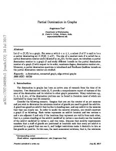
A direct consequence of this fact is that all partial 3-trees can be decomposed into an SP-graph and a forest. Thus, our edge-decomposition of a partial Matryoshka graph into an SP-graph and a forest (see Lemma 3.7) is a special case of this more general result. However, we shall now try to identify tighter decompositions for three subclasses of planar partial 3-trees: Halin graphs, IO-graphs, and partial Matryoshka graphs. In particular, we shall try to decompose these graphs into an outerplanar graph and a forest, recalling that outerplanar graphs are a strict subset of SP-graphs (by Theorems 1.7 and 1.8, or simply Theorem 1.12). By its very definition (see page 9) any Halin graph can be decomposed into a tree and a cycle. An IO-graph’s decomposition is not as obvious, but it can always be decomposed into a forest and an outerplanar graph: Lemma 4.1 Let G be an IO-graph. Then G can be decomposed into an outerplanar graph and a forest. Proof: Recalling the definition of an IO-graph, G has a planar embedding such that the vertices not on the outer-face form an independent set. Using this same planar embedding, we assign all edges in G not incident to the independent set vertices to set A. Using a cyclic labelling of the vertices on the outer-face (say, increasing in clockwise order), we define the range of an independent set vertex v to be the interval (lv , hv ), where lv is the lowest label vertex to which the independent set vertex v is adjacent, and hv is the highest. Given these ranges for all independent set vertices, we obtain a tree-like hierarchy using the property of range enclosure (i.e. since the graph is planar, there can be no overlap of ranges, only enclosure and disjointness as with Nested SAT). Now for each vertex v in the independent set, we assign to set A its edge to the vertex hv . Since the independent set vertices have degree one in edge set A and they are incident to vertices on the outer-face, then we can shift them to the outer-face without obscuring other vertices. Hence, it follows that the edges in set A induce an outerplanar graph. Thus, it only remains to show that E(G) \ A is a forest. We assume for contradiction that E(G)\A contains a cycle C. Since E(G)\A contains no edges between vertices on the outer-face, and G contains no edges between independent set vertices (by definition), then C must be a cycle of even length that alternates between vertices on the outer-face and vertices in the independent set. Let v be an independent set vertex in C such that v is not an ancestor of any other independent set vertex in C according to the range hierarchy on independent set vertices. Such a v must exist since enclosure is an acyclic property (i.e. the range hierarchy is a tree). Based on this, we can see that vertex v can only share lv and/or hv as common neighbours with other independent set vertices in cycle C. However, v is not adjacent to hv in E(G) \ A, and thus lv is a cut-vertex separating v from all other independent set vertices in C. This contradicts the fact that v is in a cycle C with these vertices, and hence we conclude that such a cycle cannot exist. Thus, E(G) \ A is a forest. 2 51
See Figure 4.1 for an example of such a decomposition. Finally, as mentioned in Chapter 3, finding a tighter edge-decomposition for partial Matryoshka graphs remains an open problem.
Figure 4.1: IO-Graph Decomposition into an Outerplanar Graph and a Forest We shall now turn our attention to decomposing graphs of unbounded treewidth. To ensure that our results are not trivial expressions of Remark 4.1, we will only be considering graph classes where k-trees (and other partial k-trees containing most edges implied by its tree decomposition) are excluded for large enough k. In particular, planar graphs and regular graphs enforce a linear relationship between m and n, and hence the additive relationship for bounded treewidth decompositions does not apply to them.
4.1.2
Decomposing Planar Graphs into Graphs of Bounded Treewidth
Every graph has an edge-decomposition into forests. The arboricity of a graph G, denoted Υ(G), is the minimum number of forests required to express G in this fashion. By Remark 1.10 it follows that the arboricity of a graph indicates the smallest k such that G is a partial (1, . . . , 1)-tree. | {z } k
l m qk Nash-Williams proved that for any non-trivial graph G, Υ(G) = maxk { k−1 }, where qk denotes the maximum number of edges in a subgraph of G containing k vertices [83, 84, 102]. By the Nash-Williams formula above and Remark 1.4, it is obvious that planar graphs have arboricity at most three, and that this bound is tight. In other words, planar graphs are a (strict) subset of partial (1, 1, 1)-trees but not a subset of partial (1, 1)-trees. Moreover, for this special case the decomposition can be found in linear time [36, 55, 96] and tightened with regards to the maximum degree of one forest [13]. 52
We also note that since any graph of treewidth p + q is a partial (p, q)-tree, then we can apply this result repeatedly to conclude that the arboricity of a graph is never greater than its treewidth: Remark 4.2 Let G be a graph of treewidth k. Then Υ(G) ≤ k.
IO-graphs forest + cycle
Nested SAT
Halin graphs
forest + outerplanar
Partial Matryoshka graphs
partial 3-trees
partial (2,1)-trees
partial (3,1)-trees Planar graphs =partial (2,2)-trees = partial (1,1,1)-trees
Figure 4.2: Planar Graph Class Hierarchy Of course, more sophisticated results have been shown. For instance, it is known that planar graphs are partial (2, 2)-trees [41, 73], and this result is also tight in terms of treewidth since planar graphs are not partial (2, 1)-trees [42]. An earlier result by El-Mallah and Colbourn had shown that planar graphs are partial (3, 3)-trees using IOgraphs to construct the decomposition [42]. We note that since outerplanar graphs have treewidth at most two, then all of these results are strongly related to the conjecture by Chartrand, Geller, and Hedetniemi that every planar graph can be decomposed into two outerplanar graphs [30]. Chartrand, Geller, and Hedetniemi had already shown that every planar graph had a vertex-decomposition into two outerplanar graphs when they made this conjecture, but it remains open today, despite claims to the opposite (e.g. [65]3 ). 3
Although I am unaware of the particular error in Heath’s paper,
53
websites such as
The Chartrand-Geller-Hedetniemi conjecture is trivial for planar graphs with a Hamiltonian cycle, since the cycle can be used to partition the graph’s edges (inside and outside the cycle) into two outerplanar graphs. Since we only need to consider triangulated planar graphs, and since 4-connected planar graphs always have a Hamiltonian cycle (Theorem 1.1), then the only types of graph to consider are (non-Hamiltonian) 3-connected triangulated planar graphs. In any case, strengthening the result from two SP-graphs to two outerplanar graphs is rather difficult. Although outerplanar and SP-graphs both have at most 2n − 3 edges, the additional structural restrictions on outerplanar graphs is significant. In this thesis, we will investigate the different, but related, problem of finding partial (k, 1)-tree decompositions.
4.2 4.2.1
Partial (k, 1)-Tree Decompositions Partial (2, 1)-Trees and Partial (3, 1)-Trees
From the infinite set of counter-examples given by El-Mallah and Colbourn [42], we know that planar graphs are not always partial (2, 1)-trees. We will show that this set of graphs does not prove that planar graphs are not partial (3, 1)-trees, but first we must recall some notation from page 34. Given triangulated planar graphs G and H with fixed planar embeddings, we use G ← H to denote the graph obtained by substituting graph H into every face of graph G. Given this notation, El-Mallah and Colbourn’s infinite set of graphs can be expressed as {HG = (((G ← K4 ) ← K4 ) ← P6 ), where G is any 5connected triangulated planar graph}. Recall from Theorem 1.12 and Figure 1.6 that K4 is a forbidden minor of partial 2-trees and the octahedral graph P6 is a forbidden minor of partial 3-trees. We shall now show that given a graph G that is a partial (3, 1)-tree, HG must also be a partial (3, 1)-tree:
Figure 4.3: Extending G’s Partial (3, 1)-Tree Decomposition to G ← K4 Lemma 4.2 Let G be a triangulated planar partial (3, 1)-tree, and let H = (G ← K4 ). Then H is a triangulated planar partial (3, 1)-tree. http://www.emba.uvm.edu/∼archdeac/problems/outplane.htm claim that the problem is unsolved. This claim is reinforced by the existence of later papers attempting to solve the conjecture, such as those by Kedlaya and Ding et al. [41, 73].
54
Proof: It is obvious that H will be planar and triangulated, so we need only argue that H is a partial (3, 1)-tree. For each face into which K4 is substituted, at most two of the edges on the boundary of this face can be in the forest of the partial (3, 1)-tree decomposition for graph G (since all three edges would create a cycle). For each of these cases, choosing appropriate edges when extending the forest ensures that the new vertex in each face is simplicial in the subgraph forming the partial 3-tree and has degree at most three (see Figure 4.3, where dashed edges represent edges assigned to the forest). Thus, by Theorem 2.2, the result holds. 2
1
3 2
1
2 3
1
2 3
Figure 4.4: Extending G’s Partial (3, 1)-Tree Decomposition to G ← P6 Lemma 4.3 Let G be a triangulated planar partial (3, 1)-tree, and let H = (G ← P6 ). Then H is a triangulated planar partial (3, 1)-tree. Proof: Once again, it is obvious that H will be planar and triangulated, so we need only argue that H is a partial (3, 1)-tree. We also know that at most two of the outer-face edges for P6 will be in the forest. We shall select our forest edges for P6 as shown in Figure 4.4 (where dashed edges represent forest edges). We can then remove the internal vertices of P6 in the order shown (see Figure 4.4), by applying the almost simplicial rule to the first vertex, and the simplicial rule to remove the other two. Since every vertex is removed when it has degree at most three, then we can conclude from Theorems 2.2 and 2.3 that H is a partial (3, 1)-tree. 2 Theorem 4.1 Let G be a triangulated planar partial (3, 1)-tree. If we define graph HG to be (((G ← K4 ) ← K4 ) ← P6 ), then HG is also a partial (3, 1)-tree. Proof: This result follows immediately from two applications of Lemma 4.2 and one application of Lemma 4.3. 2 The icosahedral graph (the smallest 5-connected triangulated planar graph) can be decomposed into a forest and an outerplanar graph, as shown in Figure 4.5. Thus, by Theorem 1.7 the icosahedral graph is a partial (2, 1)-tree, and hence a partial (3, 1)-tree. Hence, we can conclude the following: 55
Figure 4.5: The Icosahedral Graph is a Partial (2, 1)-Tree Theorem 4.2 Planar partial (2, 1)-trees are a strict subset of planar partial (3, 1)-trees. Proof: We have proven that the icosahedral graph is a partial (3, 1)-tree, and thus by applying Theorem 4.1, we conclude that at least one of the (infinite set of) graphs given by El-Mallah and Colbourn [42] is a partial (3, 1)-tree4 . However, El-Mallah and Colbourn proved that these graphs are not partial (2, 1)-trees. Thus, the result follows. 2 To summarize, we observe that planar graphs can be decomposed into three graphs of treewidth one, and into two graphs of treewidth two, but are not partial k-trees for any constant k. Thus the only remaining question is whether planar graphs are partial (k, 1)-trees for any constant k > 2 (see Figure 4.2), which we will explore in the next section.
4.2.2
Hamiltonian Planar Graphs
In this section we show that Hamiltonian planar graphs can be decomposed into a forest and graph of outerplanarity O(log n). As a consequence, we conclude that Hamiltonian 4 Indeed, we have shown that all of these graphs are partial (3, 1)-trees unless there exists a 5-connected triangulated planar graph that is not a partial (3, 1)-tree.
56
planar graphs are partial (k, 1)-trees where k is O(log n). Whether or not this outerplanarity result can be extended to all planar graphs remains an open question at this time. It also remains to be seen whether planar graphs are partial (k, 1)-trees for some constant k ≥ 3.
111111 000000 000000 111111 000000 111111 000000 111111 000000 111111 000000 111111 000000 111111
u
v
Figure 4.6: Outerplanar Sections of a Hamiltonian Graph Since any decomposition of a graph into graphs of bounded treewidth must also hold for all its subgraphs (by Theorem 1.6), then without loss of generality we need only consider triangulated planar graphs. We begin this analysis by examining Hamiltonian triangulated planar graphs. Let G denote our Hamiltonian triangulated planar graph, and let C denote its Hamiltonian cycle. Considering only edges on and outside C, we can envision this subgraph as being composed of three 2-connected outerplanar sections (see Figure 4.6)5 . Note that the edges on and within the Hamiltonian cycle form an outerplanar graph, and hence a graph of treewidth at most two (by Theorem 1.7). In order to bound the outerplanarity of this graph minus a forest, we will only select forest edges from the outerplanar sections outside of the Hamiltonian cycle. The goal is to assign edges to the forest such that all remaining edges in these outerplanar sections add at most O(log n) outerplanarity to the graph inside of the Hamiltonian cycle. We begin by introducing an algorithm that decomposes an outerplanar graph (minus one edge) into two forests with certain properties. The general idea of Algorithm 4 is to eliminate the edges that increase outerplanarity for the vertices furthest from the outerface. In order to do this, we consider the dual tree of the outerplanar section minus the outer-face (recall Remark 1.7). As we shall see, the height of the dual tree relates to the outerplanarity of the graph, and hence at each stage we simply select the edges to the child subtree of greater height. An example of the decomposition produced by this algorithm, along with the dual tree guiding this decomposition, appears in Figure 4.7. 5
Since we can select the outer-face of our planar embedding, we can guarantee that an edge on the Hamiltonian path will appear on the outer-face. In this manner we can reduce the number of outerplanar sections to two instead of three. However, this change does not simplify our proof or improve our results.
57
Algorithm 4: Decomposing a 2-Connected Outerplanar Graph Minus One OuterFace Edge Input: Internally-triangulated 2-connected outerplanar graph G with a fixed planar embedding, and two vertices u and v, adjacent on the outer-face Output: A decomposition of G − (u, v) into two forests such that neither forest has a path from u to v Let T be the dual of G Split the outer-face vertex into n pairwise non-adjacent vertices, one per edge incident to the outer-face Delete from T the (nth) outer-face vertex incident to the dual of edge (u, v) Let w denote the unique vertex in G such that u, v, w is an internal face of G Root the tree T at the face u, v, w Starting at the root and traversing the internal (non-leaf) vertices of tree T , we do the following at each vertex: Let p be the current vertex, cl its left child, cr its right child if height of cr ’s subtree cr > height of the cl ’s subtree then Colour (p, cl ) blue and (p, cr ) red else Colour (p, cl ) red and (p, cr ) blue Transfer all colours from T ’s edges to G’s edges Return R and B, the set of red and blue edges in G, respectively In greater detail, since the dual of an outerplanar graph minus the outer-face is a tree, and since we split the outer-face into n non-adjacent vertices, then the T in Algorithm 4 is also a tree (where each leaf is one of the pairwise non-adjacent outer-face vertices). Also, every edge in the outerplanar section except for (u, v) has a unique dual edge in T , and thus the edge colours can be transferred uniquely from T to G. Since the outerplanar graph G is internally-triangulated, each vertex in the tree T has exactly two children and one parent except for the root and the n − 1 leaves (outer-face vertices). The root face is not adjacent to the outer-face (since the dual of edge (u, v) is deleted), and thus it has two children and no parent. Each of the n − 1 outer-face vertices is obviously only adjacent to its parent. Finally, we note that the order in which vertices are traversed in the tree makes no difference, as subtree height is not affected by the colouring of the edges. We can now prove that the desired properties of Algorithm 4 do indeed hold: Lemma 4.4 Algorithm 4 assigns a unique colour to every edge in G except for (u, v). Proof: Every edge in G has a dual edge in T except for (u, v), and these edges are in one-to-one correspondence. Since each non-leaf vertex in T has exactly two children, and 58
u
v
Figure 4.7: Dual Tree and Resulting Decomposition by Algorithm 4 of Figure 4.6 Algorithm 4 visits each non-leaf vertex once, then each edge to a child is coloured exactly once (when its parental vertex in T is visited). 2 Lemma 4.5 Algorithm 4 returns a decomposition of G − (u, v) such that there is no single-colour path from u to v. Proof: Proof by mathematical induction on n: If G has three vertices, then edge (u, v) does not appear in the decomposition, while the two remaining edges are assigned opposite colours. Hence the claim holds for n ≤ 3. Assume the claim holds for all n < k, k ≥ 4 and consider the case where n = k. There exists a unique vertex w such that u, v, w is an internal face of G. Hence w is a cut-vertex in G − (u, v), and any path from u to v must pass through w. However, by our induction hypothesis, the only single-colour path from u to w is the edge (u, w), since the left child subtree is decomposed in the same manner as the entire tree. The same reasoning shows that the only single-colour path from w to v is the edge (w, v). However, since (u, w) and (w, v) are assigned different colours, then no single-colour path can exist from u to v. Thus the result holds for n = k. By the principle of mathematical induction, the statement is true for all n. 2 Lemma 4.6 Algorithm 4 returns a decomposition of G − (u, v) into two forests. Proof: Assume for contradiction that there is a cycle of some colour. Let e = (x, y) be the top-most edge in the cycle according to heights in the tree T . Then there is a singlecolour path from x to y in G − (u, v) − e. However, this implies that the subgraph rooted at edge e was coloured by Algorithm 4 such that it had a single-colour path between its two endpoints (not including the direct edge). However, this contradicts the results of Lemma 4.5. Thus no such cycle can exist. 2
59
Theorem 4.3 Let G be an internally-triangulated 2-connected outerplanar graph with a fixed planar embedding, and let u, v be vertices adjacent on the outer-face of G. If we delete the edge (u, v), then the resulting graph can be decomposed into two forests, such that neither forest has a path from u to v. Proof: Follows immediately from Lemmas 4.5 and 4.6.
2
Now we will show that using Algorithm 4 to decompose the three outerplanar sections of a Hamiltonian planar graph will result in a decomposition of Hamiltonian planar graphs into a forest and a graph of treewidth O(log n). The forest edges will be those marked as red, recalling that red edges were those to the subtree of greater height. Theorem 4.4 Let G be a triangulated planar graph with Hamiltonian cycle C. Assume Algorithm 4 is used to decompose each of G’s three outerplanar sections (see Figure 4.6), and returns the edges sets R1 and B1 , R2 and B2 , and R3 and B3 , respectively. Then G \ (R1 ∪ R2 ∪ R3 ) has outerplanarity at most log2 (n) + 2. Proof: We note that for any graph, the radius of its dual plus one is an upper-bound on the outerplanarity of the original graph (i.e. the face corresponding to the dual vertex of minimum eccentricity can be assigned as the outer-face). Thus, we need only consider a single outerplanar section on n vertices, and show that its dual graph has radius at most log2 n + 1. We do this by showing that the height of an outerplanar section’s dual tree (omitting the outer-face of the outerplanar section) T is at most log2 n. Since the dual of edge deletion is edge contraction, and since the forest of red edges is being deleted from graph G, then essentially Algorithm 4 contracts the edges to the child subtree of greatest height for every non-leaf vertex in T . Thus, we need only show that in a rooted tree with ≤ 2 children per node, contracting the edge to the child subtree of greatest height for every non-leaf vertex results in a tree with at most log2 n height. We prove this by induction: A tree on one node has height zero, and this equals log2 1, so the statement holds for n = 1. Assume tree T has n = k nodes, k ≥ 2, and that the statement holds for all n < k. If the root has a single child, then the edge connecting the root to that child will be contracted, and so the height of tree T is the height of the subtree, which is at most log2 (k − 1) < log2 (k) by the induction hypothesis. Thus the statement holds in this case. If tree T has two children whose subtrees have different heights, then we contract the edge to the higher sibling, and the height of tree T will be the height of this child’s subtree, which is at most log2 (k − 2) by the induction hypothesis. Again, since log2 (k − 2) < log2 (k), the statement holds. Lastly, if the root of tree T has two child subtrees of equal height, the height of tree T will be one greater than the height of its subtrees, no matter which edge is contracted. We note that the child subtree with the fewest number of vertices has at most k−1 2 vertices, indicating that it has height at most 60
log2 ( k−1 2 ) = log2 (k − 1) − 1. Since the two child subtrees have equal height, it follows that they both have height at most log2 (k − 1) − 1. Thus the height of tree T (after contraction) will be at most log2 (k − 1) < log2 (k). Thus, the statement holds for all cases and, by the principle of mathematical induction, for all n. Hence, we conclude that Algorithm 4 decomposes each outerplanar section such that its dual has radius at most log2 n + 1. In other words, each outerplanar section will have outerplanarity at most log2 n + 2, as desired. 2 We note that the concept of a compressed tree with O(log n) height in Harel and Tarjan’s paper [62] is quite similar, although not identical, to our contracted tree above. Similar ideas have also appeared in papers on set union [99] and algorithms relating to nearest common ancestor [1]. Now, having proved such a decomposition exists for planar graphs containing a Hamiltonian cycle, the question remains as to how efficiently we can find this decomposition. The dual of a planar graph can be computed in O(n + m) time, and given the Hamiltonian cycle, we can identify the outerplanar sections in linear time. Thus we can also compute a dual tree for each outerplanar section in linear-time. For each of these (at most three) outerplanar sections, we can compute the height of each node in linear-time using a simple postorder traversal. Thus we can identify which dual edges to contract in linear-time, and this corresponds to identifying the decomposition of the original graph in linear-time. Hence, we can conclude the following: Theorem 4.5 Given a triangulated planar graph G and a Hamiltonian cycle C in G, we can decompose G into a partial (k, 1)-tree with k ∈ O(log n) in linear time. Finally, although finding a Hamiltonian cycle on planar graphs is N P-complete on 3connected graphs, a linear-time algorithm exists when we restrict ourselves to 4-connected planar graphs ([33, 50], recall Theorem 1.1). We can also triangulate a planar graph in linear time. Thus, we obtain the following result as well: Theorem 4.6 Given a planar 4-connected graph G, we can decompose G into a partial (k, 1)-tree with k ∈ O(log n) in linear time. The obvious next step is to see whether or not this result extends to all 3-connected triangulated planar graphs, as this would prove the existence of such a decomposition for all planar graphs. However, as we shall see, this result cannot easily be extended to such graphs. If we have a 3-connected triangulated planar graph G, we can construct a tree of 4connected components to represent this graph, with nodes representing 4-connected components and edges connecting 4-connected components with a 3-separating set in common 61
1 0 0 1
11 00 00 11
11 00 00 11
11 00 00 11
1 0 0 1 0 1 1 0 0 1 0 1 1 0 0 1 0 1 11 00 00 11 00 11
11 00 00 11 00 11
1 0 0 1 0 1
11 00 00 11
1 0 0 1
1 0 0 1 1 0 0 1 0 1
1 0 0 1
1 0 0 1
1 0 0 1 0 1
1 0 0 1
Figure 4.8: 3-Connected Graph and its Tree of 4-Connected Components (see Figure 4.8). Using the decomposition method for Hamiltonian planar graphs we can derive a treewidth decomposition for each 4-connected component, but the problem is in combining these decompositions. Since graph G is triangulated, the 3-separating set must form a triangle (i.e. a cycle of length three), and thus one of the questions is whether or not the 4-connected components containing this triangle agree on its decomposition. If we root this tree of 4-connected components, then we can have each parent component impose its decomposition onto its children. Since each 4-connected component will have to alter its bounded treewidth decomposition for a single parent, and since this alteration affects a constant amount of edges (since a single triangle is being imposed), then the increase in treewidth is at most a constant for each 4-connected component. In other words, we can identify a forest in G such that each 4-connected component within G is decomposed into a partial (k, 1)-tree for some k ∈ O(log n). Unfortunately, combining the tree decompositions for each 4-connected component’s partial k-tree is problematic. If zero or two of the triangle’s edges are assigned to the 62
partial 1-tree, then the separating triangle is a clique of size three or one, respectively. In this case, a simple clique sum combines the tree decompositions without increasing treewidth. However, if exactly one of the separating triangle’s edges is assigned to the forest, then there is no guarantee that these tree decompositions can be merged without increasing treewidth. Furthermore, this problematic case cannot be avoided within every separating triangle without increasing the treewidth of these decompositions. Thus, our decomposition result is limited (for now) to 4-connected and Hamiltonian planar graphs.
4.2.3
Consequences
In conclusion, although the problem of decomposing planar graphs into a forest and partial k-tree for some constant k remains open, we give a decomposition for Hamiltonian planar graphs that bounds outerplanarity to O(log n). Consequently, we can solve most N Phard problems on the partial k-tree part of this decomposition in O(2k n) = O(n2 ) time, which can help in the construction of approximation algorithms for this graph class, as we shall see in Chapter 5.
4.3
Restricted Decompositions of Bounded Treewidth
We now explore restricted decompositions of graphs into partial (k, 1)-trees. In particular, we add the restriction that the forest has maximum degree one. In other words, it is a matching (i.e. a set of pairwise non-adjacent edges, see page 3). We extend our current notation by denoting matchings as partial 1/2-trees.
4.3.1
Cubic Graphs are Partial (k, 1/2)-trees
We begin by proving that cubic graphs can be decomposed into a matching and graph of treewidth at most two. We begin with the following well-known theorem: Theorem 4.7 Petersen’s Theorem: Every cubic bridgeless graph has a perfect matching [86]. Thus, for cubic bridgeless graphs, the problem is essentially solved: Lemma 4.7 A graph with maximum degree two has treewidth at most two. Proof: A connected graph with maximum degree two is either a path or a cycle. The former has treewidth one, while the latter has treewidth two. Thus the result follows for all such graphs. 2
63
Theorem 4.8 Every cubic bridgeless graph is a partial (2, 1/2)-tree. Proof: Let G be a cubic bridgeless graph. By Theorem 4.7, G has a perfect matching M . Since every vertex in G is covered by M , then G − M is a graph of maximum degree two. The result follows from Lemma 4.7. 2 In order to extend the result to all cubic graphs, we first make the following observations: Lemma 4.8 Let G be a graph containing one or more cycles (i.e. not a forest). Let H be the graph obtained by deleting all bridges in G. Then tw(H) = tw(G). Proof: Adding an edge between two separate components cannot increase treewidth, unless neither component had an edge (since this is a clique sum). Thus, so long as some component of H contains an edge, the result will follow. However, this must be true since G had a cycle. 2
Figure 4.9: Components after Bridge Deletion Thus our algorithm for decomposing cubic graphs into a matching and partial 2-tree begins with the deletion of all bridges. We note that any vertex incident to two bridges must be incident to three (if any incident edge is on a cycle, at least two of them must be). Thus the resulting components are either isolated vertices or components containing vertices of degree three and two (see Figure 4.9). Isolated vertices obviously have treewidth less than two, so we only need consider components containing cycles. Let C be such a component, and let d represent the number of vertices of degree two in C. We shall now argue that for every d > 0, we can construct a matching that covers all vertices of degree three. Thus, by Lemma 4.7, such components are partial (2, 1/2)-trees. 64
Figure 4.10: Components with Three or More Vertices of Degree Two Lemma 4.9 Let G be a connected graph with d ≥ 3 vertices of degree two, and n − d vertices of degree three. Then there exists a matching that covers all vertices of degree three. Proof: Since d ≥ 3, we can add d − 2 new cubic vertices to graph G in order to create a cubic bridgeless graph H (see Figure 4.10). Having added such vertices and edges, we can find a perfect matching MH for H, and then identify the subset of that matching contained within the original graph G (i.e. MG = {e : e ∈ MH ∩ E(G)}). MG must cover all vertices of degree three in G, since all vertices in G are covered by MH , and no vertex of degree three in G is incident to any edges in E(H) \ E(G). Hence we conclude that G − MG is a graph of maximum degree two. 2 Lemma 4.10 Let G be a connected graph with d = 2 vertices of degree two, and all other vertices of degree three. Then there exists a matching that covers all vertices of degree three. Proof: There exists a stronger version of Petersen’s Theorem (Theorem 4.7) such that cubic bridgeless multigraphs (that is, graphs where E is a multi-set rather than a set) have perfect matchings (refer to [20] for details and applications). Thus, we can simply connect the two vertices of degree two with a new edge, and find a perfect matching MH for this new graph H. Once again, we can obtain the subset of MH on graph G, which we denote as MG . Since only the two vertices of degree two may no longer be matched, then we conclude that G − MG has maximum degree two (see Figure 4.11). 2 For this last proof we require the concept of a tree of 2-connected components. Recall from page 62 that a tree of k-connected components is formed by representing each kconnected component of the graph as a node, and connecting two nodes if and only if their respective components have some vertices in common (i.e. a separating set in the original graph of size at most k − 1). Thus, for a tree of 2-connected components, each 65
Figure 4.11: Components with One or Two Vertices of Degree Two 2-connected component of a graph would be represented by a node, and two nodes would be adjacent if and only if they shared a common cut-vertex. We can now proceed with the proof. Lemma 4.11 Let G be a connected graph with a single vertex v of degree two, and all other vertices of degree three. Then there exists a matching that covers all vertices of degree three. Proof: There exists a stronger version of Petersen’s Theorem (Theorem 4.7) which states that cubic graphs have a perfect matching if their tree of 2-connected components forms a path [20]. Thus, if we create a copy of graph G, and connect v to its copy, we create a cubic graph H with a single bridge (see Figure 4.11). In other words, the tree of 2-connected components is K2 , which is certainly a path. Hence there exists a perfect matching MH on this new graph H, and we can identify the subset MG of this matching on graph G. Since only vertex v is incident to edges in E(H) \ E(G), then it follows that every degree three vertex in graph G is covered by MG . Hence, the result follows. 2 We can now apply these Lemmas to conclude the following: Theorem 4.9 Let G be a graph of maximum degree three. Then G is a partial (2, 1/2)tree. Proof: The case where G is cubic is handled by Theorem 4.8. Thus, without loss of generality we assume that G has one or more bridges. Using Lemma 4.8, we delete all bridges without affecting treewidth. Each resulting component is either an isolated vertex or a component with d > 0 vertices of degree two and all other vertices of degree three. In the second case, we can apply Lemmas 4.9, 4.10, and 4.11 accordingly in order to obtain a matching for each component that covers all vertices of degree three. It follows from Lemma 4.7 that each component is a partial (2, 1/2)-tree or an isolated vertex (i.e. of treewidth zero). Since every component is a partial (2, 1/2)-tree or isolated vertex, assigning the bridges of G to the partial 2-tree does not increase the treewidth,
66
by Remark 1.9, since it is a clique sum of size one. Thus, we conclude that G must be a partial (2, 1/2)-tree. 2 We note that if our partial (2, 1/2)-tree decomposition of a graph results in a partial 2tree with more than one component, then edges should be transferred from the matching back to the partial 2-tree until it is connected (i.e. without increasing treewidth, by Remark 1.9). This reduces the number of edges in the matching, which will be beneficial for our algorithms, as we shall see in Chapter 5.
4.3.2
Maximum Degree Three is Tight
We now prove that planar graphs of higher degree are not partial (k, 1/2)-trees for any fixed k. We do so by constructing a planar graph that will contain the k × k rectangular grid graph as a minor no matter how one selects the matching. Since this grid graph has treewidth k and we can construct such a planar graph for any fixed k, the result immediately follows. Indeed, our result holds for planar graphs of maximum degree four, thus proving that maximum degree three is tight.
Figure 4.12: 8 × 8 Rectangular Grid Graph Let Dk represent the graph constructed by replacing each edge in a k × k rectangular grid graph with two triangles (forming a diamond shape, see Figure 4.13). The resulting graph is certainly planar and, as we shall argue, must contain the original grid graph as a minor, no matter how one selects the matching. Lemma 4.12 Let k be any positive integer. Then Dk+1 is not a partial (k, 1/2)-tree. Proof: For each cycle of length three (i.e. triangle) in Dk+1 , at most one edge on the cycle can be in the matching. Hence, the vertices of a triangle remain in the same component after the deletion of any matching. The diamond shape (see Figure 4.13) consists of two 67
triangles, and hence the two original endpoints (the two vertices not common to both triangles) are connected by a path using only diamond vertices and edges, even after the deletion of any matching6 . By contracting this path (and deleting any unnecessary edges in the diamond shape), we obtain a single edge joining the two endpoints of the diamond shape. By doing this for every diamond in the graph, we obtain the (k + 1) × (k + 1) rectangular grid graph as a minor. In other words, deleting any matching from Dk+1 results in a graph of treewidth ≥ k + 1 by Theorem 1.6. 2
Corollary 4.1 Planar graphs are not partial (k, 1/2)-trees for any constant k. Proof: We need only show that Dk is planar for any integer k > 0. Since the rectangular grid graph is planar, and substituting the diamond shape for each edge does not make the graph non-planar, the result follows. 2
Figure 4.13: D8 and the Diamond Formation Since we know that planar graphs in general are not partial (k, 1/2)-trees yet cubic planar graphs are, the question arises as to where the cutoff is in terms of maximum degree. We shall now show that planar graphs with maximum degree ≥ 4 are not always decomposable into a matching and partial k-tree for any fixed k. In other words, the result on cubic graphs is tight. Lemma 4.13 Planar graphs with maximum degree at least four are not partial (k, 1/2)trees for any constant k > 0. Proof: We employ the same argument as before, but we use a slightly different substitution. More specifically, each vertex is replaced by two triangles with a single vertex 6 We can see here that a single triangle would have sufficed. However, we chose the diamond shape for symmetry.
68
in common, which we denote as an inverted diamond, and each edge is replaced with a diamond (see Figure 4.14). Note that each diamond is attached to a distinct vertex (not common to both triangles) on the inverted diamond. Once again, it is clear that this substitution does not make the graph non-planar, and the use of triangles ensures that the deletion of any matching cannot eliminate the path between two vertices that were adjacent in the original grid graph. Hence, once again we can construct a graph that contains the (k + 1) × (k + 1) rectangular grid graph as a minor (for any constant k) after the deletion of any matching. Finally, this modified substitution produces a graph with maximum degree four. Thus the result follows. 2
Figure 4.14: Modified Grid Graph of Maximum Degree Four The purpose of using matchings was to bound the maximum degree of the forest. Although this technique worked on cubic graphs (planar and non-planar), it could not be extended to graphs of higher degree, even when restricted to planar ones. If we loosen this bound to two or some higher constant (e.g. if the forest is a set of vertex-disjoint paths instead of a matching), can we then decompose graphs of higher maximum degree (planar or otherwise)? Perhaps Eulerian paths could help construct appropriate decompositions for quartic graphs, but this remains an open question at this time. However, this bound on the maximum degree of the forest is desirable since it helps in the development of algorithms using these decompositions, as we shall see in Chapter 5.
4.4
Decompositions into a Bipartite Graph and Forest
It has been proven that planar graphs can be decomposed into two bipartite graphs [61, 59, 80]. One question that arose in our research is whether planar graphs can be decomposed into a bipartite graph and a forest (note that a forest is bipartite since it contains no (odd) cycles, by Remark 1.3). This question does not relate directly to our 69
decompositions of bounded treewidth, since bipartite planar graphs can have unbounded treewidth (e.g. rectangular grid graphs). However, such a proof would be a strengthening of the Four Colour Theorem [59, 61, 80] and can also be used for approximation algorithms (see Chapter 5). Although the result was unpublished, Seymour answered this question in the negative in private discussions with Rick Mabry [81]. However, the result does hold for some types of planar graphs, which we explore below. We begin by exploring graphs of bounded treewidth, and we find that our first result does not require the graph to be planar: Theorem 4.10 Let G be a partial 3-tree. Then G can be decomposed into a bipartite graph and forest. Proof: Since G is a partial 3-tree, then it is the subgraph of a 3-tree, say H. Let v1 , . . . , vn be the perfect elimination order of H. Then we can greedily 4-colour H using the perfect elimination order. Because the predecessors of a vertex form a clique, then each vertex’s predecessors are assigned a unique colour. We can use this 4-vertexcolouring to assign the edges of H to three different sets (i.e. set A contains edges in E(H) whose endpoints are colours 1 and 2 or colours 3 and 4, set B contains edges whose endpoints are colours 1 and 3 or 2 and 4, and set C contains all other edges in E(H)). We claim that H[A] is a forest and H[B ∪ C] is a bipartite graph. The second half of this claim follows immediately from the definition of these edge sets since H[B ∪ C] does not contain any edges between vertices of colour 1 and 2, nor edges between vertices of colour 3 and 4. Thus we only need to prove the claim that H[A] is a forest. Assume (for contradiction) that a cycle exists. Then choose the last vertex in the cycle according to the perfect elimination order. This vertex must have two predecessors of the same colour, contradicting the properties of our vertex colouring. Hence the assumption cannot hold, and H[A] is a forest. Since H can be decomposed into a bipartite graph and forest, the same holds for its subgraph G. 2 Restricting the above result to planar partial 3-trees cannot make it false, thus we conclude the following: Corollary 4.2 Let G be a planar graph of treewidth at most three. Then G can be decomposed into a bipartite graph and a forest. For instance, applying the above method to the partial 3-tree from Figure 1.1, we obtain the perfect elimination ordering v11 , v5 , v3 , v7 , v12 , v10 , v1 , v2 , v4 , v9 , v8 , v6 , v13 , v14 , v15 , which results in the following 4-vertex-colouring: ({v1 , v9 , v11 , v13 , v15 }, {v2 , v5 , v10 , v14 }, {v3 , v6 , v8 }, {v4 , v7 , v12 }).
70
v8
v7 v6 v9 v2 v1
v5
v4
v3
v10 v11
v13 v15
v12 v14
Figure 4.15: Partial 3-Tree Bipartite-Forest Decomposition Thus we obtain a decomposition of this partial 3-tree into a bipartite graph and forest, as shown in Figure 4.15. However, we wish to construct decompositions enabling efficient algorithms for N Phard problems and, as previously mentioned, such algorithms already exist for graphs of bounded treewidth. Thus Theorem 4.10 cannot be used to construct more efficient algorithms, although it does highlight the following piece of information: Lemma 4.14 A graph G can be decomposed into a bipartite graph and a forest if and only if it has a 4-vertex-colouring (using colours 1, 2, 3, and 4) such that there are no (even) cycles containing only colours 1 and 2 or only colours 3 and 4. Proof: ⇒ Assume graph G is decomposed into a bipartite graph B and a forest F . Then we can 2-vertex-colour both B and F , using colours a, b and c, d respectively. We can then construct a 4-vertex-colouring for G using the cross-product of these two colourings (i.e. a vertex coloured with colour a in B and colour c in F is now assigned the colour (a, c), and so on). We note that if there are any 2-coloured cycles in G, they must be of even length. Furthermore, the colours (a, c) and (a, d) cannot form a 2-coloured cycle, since the alternation of colours implies that every edge in the cycle is in the forest F , which is a contradiction. Similarly, there cannot be any 2-coloured cycles on (b, c) and (b, d). Renaming colours (a, c), (a, d), (b, c), (b, d) with colours 1, 2, 3, 4 respectively results in the desired conclusion.
71
⇐ Assume G has a 4-vertex-colouring such that there are no 2-coloured cycles on colours 1 and 2 and colours 3 and 4. Then we assign all 1 − 2 and 3 − 4 edges to set F , and all other edges to set B. F is clearly a forest by definition, and partitioning the vertices of G into those coloured 1 and 2 and those coloured 3 and 4 makes it apparent that B is bipartite. Hence G can be decomposed into a bipartite graph and a forest. 2 Based on this result, it seems likely that 3-colourable planar graphs can be decomposed into a bipartite graph plus forest. Indeed, to prove this result we need only introduce colour 4 to re-colour some vertices of colour 1 and 2 such that: 1. all cycles of colour 1 and 2 are eliminated, and 2. no cycles of colour 3 and 4 are introduced
Figure 4.16: The Tutte Graph We note that a consequence of Seymour’s proof is that such a decomposition cannot exist for all Hamiltonian planar graphs, an example being the dual of the Tutte graph [81]. 72
Other interesting questions include whether or not treewidth three is tight and, if the statement does not hold for all 3-colourable planar graphs, whether it holds for trianglefree planar graphs (a proper subset of 3-colourable planar graphs [56]).
73
74
Chapter 5
Algorithms using Bounded Treewidth Decompositions In this chapter we discuss an application of bounded treewidth decompositions: namely, the development of approximation algorithms for N P-hard problems on graph classes of unbounded treewidth. We provide an overview of the approximation classes and the status of certain graph-theoretic problems, and review the contributions of existing algorithms that use bounded treewidth decompositions. Finally, we introduce some basic algorithms that use the decompositions we have been developing.
5.1
Approximation Complexity Classes
The question as to whether P = N P is still the most important open question facing computer scientists today. Given the extreme difficulty, and likely impossibility, of finding a polynomial-time algorithm for an N P-hard problem, it makes sense to approach such problems with heuristics or approximation algorithms. In order to compare approximation methods, some proof of the closeness to optimality is necessary, and thus approximation complexity classes have developed [48, 68, 70]. We will concern ourselves with both the maximum error possible, as well as the expected error. Given that the optimal solution is of size k, we say an algorithm has an approximation factor ≤ ǫ if the solution it returns is guaranteed to be ≤ (1 + ǫ)k (for minimization problems1 ). An approximation scheme is a class of algorithms A such that for any given ǫ > 0, there exists a corresponding algorithm Aǫ that has an approximation factor of at most ǫ. If for any fixed ǫ the running time of Aǫ is polynomial in n, 1 Maximization problems can be converted to minimization problems, and hence need not be considered separately.
75
the size of the input, then we say that the class of algorithms A is a polynomial-time approximation scheme (PTAS). If we have the stronger condition that the running time of Aǫ is polynomial in n and 1/ǫ, then we say that the class of algorithms A is a fully polynomial-time approximation scheme (FPTAS). Of course, not all optimization problems allow arbitrarily-close approximations. If an optimization problem allows approximation within a constant factor in polynomial-time, then it said to be in the approximable (APX) class. Unless P = N P, it is known that there are problems in APX that are not in PTAS, and we call these algorithms APX-hard [68]. Similarly, there are PTAS-hard problems that do not permit an FPTAS. Thus we have the following hierarchy, with the inequalities holding if P = 6 N P: F P T AS ⊂ P T AS ⊂ AP X.
5.2
Status of Independent Set and Vertex Cover
Recall from Chapter 1 that an independent set is a set of vertices no two of which are adjacent, and that a vertex cover is a set of vertices such that every edge in the graph is incident to some vertex in the cover. It is obvious that the empty set and V (G) are an independent set and vertex cover, respectively, for all graphs G. However, the problem of finding the maximum independent set or minimum vertex cover of a graph is N P-hard, even when restricted to cubic planar graphs [49]. These two problems are strongly related since the complement of an independent set is always a vertex cover (i.e. an edge cannot have both endpoints in the independent set, thus each edge is incident to a vertex not in the independent set, which satisfies the definition of a vertex cover), and thus finding the maximum independent set is equivalent to finding the minimum vertex cover. The difficulty of approximating these problems depends on which graph class we consider2 . For planar graphs, both problems are in PTAS [12]. However, both problems become APX-complete on graphs with bounded ∆(G) ≥ 3. That is, they can be approximated within a constant factor, but there does not exist any polynomial-time approximation scheme unless P = N P [2, 17, 85]. The lower bounds on the approximation factors for independent set are 1.0005 for ∆(G) = 3, 1.0018 for ∆(G) = 4, and 1.0030 for ∆(G) = 5 [18]. It is approximable log log ∆(G) within ∆(G)+3 for small ∆(G), and within O( ∆(G)log ) for large ∆(G) [3, 17, 71]. 5 ∆(G) In general, independent set is not approximable within n1/2−ǫ , ǫ > 0 [64]. For vertex cover, the problem is approximable within 7/6 for ∆(G) = 3, not approximable within 1.0029 for ∆(G) = 5, and not approximable within 7/6 for large enough 2
These results were mostly gathered from the online compendium http://www.nada.kth.se/∼viggo/wwwcompendium/wwwcompendium.html.
76
found
at
Table 5.1: Approximating Independent Set and Vertex Cover Graph Class Independent Set Vertex Cover Planar ∈ PTAS ∈ PTAS ∆(G) = 3 APX-com., ǫ ≥ 0.0005 APX-com., ǫ ≤ 1/6 ∆(G) = 4 APX-com., ǫ ≥ 0.0018 APX-com. ∆(G) = 5 APX-com., ǫ ≥ 0.003 APX-com., ǫ ≥ 0.0029 Small ∆(G) APX-com., ǫ ≤ ∆(G)−2 APX-com. 5 ∆(G) log log ∆(G) ) APX-com., ǫ ≥ 1/6 Large ∆(G) APX-com., ǫ ≤ O( log ∆(G) log n All graphs 6∈ APX APX-com., 1/6 ≤ ǫ ≤ 1 − log 2 log n ∆(G) [17, 18, 34, 63]. A simple and elegant greedy algorithm (select an arbitrary edge, add both endpoints to the cover, delete all incident edges, and repeat until no edges remain) is guaranteed to return a vertex cover no larger than twice the minimum possible log n size on all graphs. This has been tightened to 1 + ǫ ≤ 2 − log 2 log n , where n is the number of vertices [14, 82]. We summarize these results in Table 5.1. We will also be considering the weighted generalizations of these problems, where the vertices are assigned positive real weights, and we must find the maximum weight independent set/minimum weight vertex cover. Thus we need to highlight some of the progress made for this variation as well. The PTAS that exists for planar graphs also applies to the weighted versions of both these problems [12]. As well, the approximation log n within a factor of 2 − log 2 log n for vertex cover in general also holds for weighted vertex cover [14, 82]. As for independent set, the weighted version can be approximated within a factor of 3/2 on graphs with ∆(G) = 3, and within ∆(G)+2 for ∆(G) > 3 [58, 67]. 3 Since the weighted versions of both these problems have a PTAS for planar graphs, we shall focus our attention on producing approximation algorithms for graphs of bounded degree. However, before proceeding with our own algorithms, we shall now review some existing algorithms that use bounded treewidth decompositions to perform tasks efficiently.
5.3
Existing Algorithms using Bounded Treewidth Decompositions
Recalling that arboricity is essentially a decomposition into partial 1-trees, Chiba and Nishizeki have developed a subgraph-listing algorithm whose efficiency relates to bounded treewidth decompositions [32]. A similar use is found in Eppstein’s paper on listing maximal complete bipartite subgraphs [44]. A more obvious application of bounded treewidth decompositions is Baker’s development of a PTAS for problems on planar graphs, such as independent set and vertex cover [12]. Baker’s method is to decompose a planar graph 77
into n/k overlapping k-outerplanar graphs. Since k-outerplanar graphs have treewidth at most 3k − 1 (recall Theorem 1.7), then most N P-hard problems can be solved on these subgraphs. It can easily be shown that the best answer among these n/k solutions is at most a factor of 1/k away from optimal. Eppstein has also developed algorithms using bounded treewidth decompositions, and generalized Baker’s approach to decompositions of graphs with locally-bounded treewidth [45, 46]. Further improvements were recently made by Demaine et al. [38].
5.4 5.4.1
Approximation Algorithms for Partial (k, 1)-Trees General Approach
Our algorithmic approach for partial (k, 1)-trees will be to use the partial k-tree decomposition to solve the N P-hard problem exactly on the subgraph of treewidth k in linear time, and then to use the partial 1-tree to adjust this solution appropriately. We note that this approach will also work on graphs that have a decomposition into a bipartite graph and forest, subject to the restriction that the N P-hard problem can be solved efficiently on bipartite graphs (e.g. independent set [76]). However, we shall confine our attention to algorithm design for decompositions of bounded treewidth.
5.4.2
Basic Approximation Algorithms
Assuming that we have a partial (k, 1)-tree decomposition for some fixed k, then we can apply the following basic algorithm: Algorithm 5: Approximating Independent Set on Partial (k, 1)-Trees Input: A partial (k, 1)-tree decomposition for graph G, for some fixed constant k Output: An independent set for G Compute the maximum independent set I for the partial k-tree Take the partial 1-tree, delete all edges that do not have both endpoints in I, and define the resulting graph to be F Compute the minimum vertex cover C of F Return R = I \ C The maximum independent set and minimum vertex cover can be computed for a graph of treewidth x in O(2x n) time [90]. This is equivalent to linear time if x is a fixed constant (i.e. k or 1). Thus steps 1 and 3 take linear time. Step 2 iterates through all edges in the forest, and hence also takes O(n) time. Finally, step 4 can be implemented in linear time. Thus this is a linear-time algorithm.
78
However, this is an approximation algorithm, so we must also examine how accurately we approximate the maximum independent set. To do so, we must first review some wellknown graph properties: Theorem 5.1 Tur´ an’s Theorem: A graph on n vertices and m edges has an independent n2 set of size at least ⌈ 2m+n ⌉. [100]. Since we are considering regular graphs, the following corollary will be important to our analysis: Corollary 5.1 Every graph with n vertices and average vertex degree k contains an inn ⌉. dependent set of size ≥ ⌈ k+1 Thus, cubic graphs have an independent set of size at least ⌈n/4⌉. Bipartite graphs— including forests, by Remark 1.3—must have a maximum independent set of size at least n/2, since we can simply pick the larger half of the bipartition. We note that this second observation also holds for the weighted version of maximum independent set. Returning to Algorithm 5, we see that step 1 computes the maximum independent set for the partial k-tree, but the next three steps correct for the fact that the edges in the partial 1-tree were not considered. Thus the initial set I is clearly an upper-bound on the maximum independent set for G, and the minimum vertex cover is computed on a forest whose number of vertices is at most |I|. Since the minimum vertex cover of a forest on n vertices is at most n/2 vertices, then we delete at most |I|/2 vertices. Hence, the independent set R that we return is at least 1/2 of the optimal size. This analysis also holds for the weighted version of maximum independent set, since set I will still be the maximum for the partial k-tree, and the partial 1-tree will select a vertex cover of at most half the weight (i.e. the smaller weighted half of the bipartition is an upper-bound on C). A similar algorithm allows us to approximate vertex cover (directly) on partial (k, 1)trees: Algorithm 6: Approximating Vertex Cover on Partial (k, 1)-Trees Input: A partial (k, 1)-tree decomposition for graph G, for some fixed constant k Output: A vertex cover for G Compute the minimum vertex cover C1 for the partial k-tree Take the partial 1-tree, delete all edges that are incident to a vertex in C1 , and define the resulting graph to be F Compute the minimum vertex cover C2 of F Return R = C1 ∪ C2
79
By the same reasoning, this algorithm also takes linear time, so we only need to consider the approximation factor. The set C1 is optimal for the partial k-tree, and hence a lower bound on the minimum vertex cover size for graph G. Since no vertex in C1 can be incident to an edge in F , then in the worst-case F will be a tree on n − |C1 | vertices. 1| 1| Thus |C2 | is at most n−|C . So we conclude that R is at most |C1 |+ n−|C = n/2+|C1 |/2 2 2 n+|C1 | vertices. In other words, our approximation factor is no worse than 2|C1 | . Although this does not give us a constant factor for all planar graphs, a simple edge-counting argument for regular graphs proves that a vertex cover includes at least half of the vertices, giving us an approximation factor of at most 3/2. A better way of analyzing Algorithm 6 is to notice that a vertex cover on the partial k-tree and a vertex cover on the partial 1-tree are both lower-bounds on the size of a minimum vertex cover. Since |C1 | corresponds to this first bound, and |C2 | is no larger than this second bound, then we conclude that |C1 | + |C2 | is at most twice the optimal size. In other words, our approximation factor is never worse than 2. We can combine these results for independent set and vertex cover, since Algorithms 5 and 6 are essentially equivalent. That is, finding the maximum independent set and minimum vertex cover for the partial k-tree will return complementary vertex sets. In both cases, F is defined to be the subset of partial 1-tree edges not covered by the vertex cover, or equivalently, incident to two independent set vertices. Lastly, in both cases we identify the minimum vertex cover of F and transfer these vertices from the independent set to the vertex cover. Thus, our approximation bounds on Algorithm 6 also apply to Algorithm 5, and vice-versa. Thus from now on we shall only discuss Algorithm 5. Finally, although Algorithm 5 claims that k must be a fixed constant, the algorithm remains polynomial-time when k ∈ O(a log(n) + b) for constants a and b, since O(2k n) = O(2b na+1 ) ∈ P. Thus we obtain the following Theorem: Theorem 5.2 Assume G is a graph class that can be decomposed into partial (k, 1)-trees, where k ∈ O(a log(n)+b) for some fixed constants a and b. Let us also say that Algorithm 5 is performed on graph G ∈ G, and returns the solution (I, C), where I is an independent set and C is its complementary vertex cover. Then we can conclude that the optimal solution (weighted or unweighted) (I ∗ , C ∗ ) has the property that |I ∗ |−|I| = |C|−|C ∗ | = ∆ and that ∆ ≤ min{|I|, |C|/2}. Furthermore, this approximate solution can be computed in linear time when k is a constant independent of n (i.e. a = 0), and polynomial time otherwise. Looking at Table 5.1 and the results for the weighted versions of these problems, we can see that our algorithm does not improve on the best-known results for graphs with maximum degree three. However, if regular graphs of higher degree are also partial (k, 1)-trees for k ∈ O(log n), then our approach will offer a better approximation for these graph classes. 80
Finally, we note that by reducing the number of edges in the forest F , we can automatically improve our approximation factor for both of these algorithms, since the vertex cover of a graph can never be larger for a subgraph (i.e. the adjustment factor can only decrease by reducing the partial 1-tree). Thus, there are significant benefits to constraining the treewidth decompositions in ways that decrease the number of edges in the partial 1-tree. For instance, using a matching when possible, transferring as many edges as possible from the forest to the partial k-tree, and even using a non-minimal k for the partial (k, 1)-tree decomposition, thereby increasing the number of edges that can be transferred to the partial k-tree.
5.5
Sample Performance
Figure 5.1: A Perfect Matching for the Tutte Graph We will now show how Algorithm 5 performs on the Tutte graph. We begin by finding a perfect matching for this cubic graph in order to decompose it into a partial (2, 1/2)-tree (see Figure 5.1). In order to reduce the number of adjustments that will be required, we should transfer 81
some of the matching edges back into the partial 2-tree. In particular, bridges and edges covered by the tree decomposition should not be kept in the matching. Adding back such edges (seven of them) in the Tutte graph, we get the partial 2-tree and its maximum independent set, as shown in Figure 5.2.
1 0 0 1 1 0 0 1
1 0 0 1
1 0 0 1
1 0 0 1 1 0 0 1
1 0 0 1 1 0 0 1 1 0 0 1
1 0 0 1
1 0 0 1
1 0 0 1
1 0 0 1
1 0 0 1
1 0 0 1 1 0 0 1
1 0 0 0 1 1 0 1
1 0 0 1
1 0 0 1
1 0 0 1
1 0 0 1 Figure 5.2: A Maximum Independent Set for the Tutte Graph’s Partial 2-Tree Since the partial 2-tree has a maximum independent set of size 22, it follows that the Tutte graph cannot have an independent set of size greater than 22. Furthermore, four of the matching edges create a conflict with the above independent set (see the dashed edges in Figure 5.2), so our algorithm returns a maximum independent set of size 18. Thus we can conclude that our algorithm returns a maximum independent set that is, at worst, 18/22 of the optimum solution (an error margin of approximately 22%). However, it can be verified that the Tutte graph actually has a maximum independent set of size 19, and thus our algorithm’s error is actually < 6% for this example. However, it should be noted that the solution for the partial 2-tree is not unique, and other answers can result in a smaller independent set (e.g. of size 17, for instance).
82
Chapter 6
Conclusion In summary, we used the concept of treewidth to simplify and extend the results by Knuth, and Kratochv´ıl and K˘riv´ anek relating to nested satisfiability. This observation demonstrated that a restricted form of graph construction was associated with treewidth at most three, and that the tree decomposition could easily be constructed from this structure. We then identified that this class could be extended even further to include more planar partial 3-trees, thereby creating a new class of nested graphs, which we named partial Matryoshka graphs. We showed that partial Matryoshka graphs were a strict subset of planar partial 3-trees whose standardized tree decomposition had at most two children per node (i.e. binary planar partial 3-trees), and that the induced graphs of such tree decompositions were always Hamiltonian. We also demonstrated that partial Matryoshka graphs, although not closed under minors, contained many planar graph classes of treewidth at most three (besides Nested SAT graphs) including outerplanar graphs, Halin graphs, and IO-graphs. We determined that the structure of partial Matryoshka graphs allowed for a simple vertex decomposition into a forest and an outerplanar graph, as well as an edge decomposition into a forest and an SP-graph. Tighter decompositions were identified for both Halin and IO-graphs. Our observations directed us towards other mathematical results relating to decompositions of bounded treewidth, such as the research surrounding the conjecture by Chartrand, Geller, and Hedetniemi, as well as the concept of arboricity and the identification of partial (p + q)-trees as partial (p, q)-trees for all p, q. Hence, we focused on planar graphs and summarized the known relationships between graphs of bounded treewidth and graphs with decompositions of bounded treewidth. Having summarized the known relationships for planar graphs, we then attempted to answer the open question as to whether or not planar graphs are partial (k, 1)-trees for some constant k. We developed an efficient algorithm which produced such a decomposition for 4-connected planar graphs with k ∈ O(log n), and demonstrated obstructions 83
to generalizing this approach to 3-connected planar graphs. We also examined decompositions of bounded treewidth for graphs of bounded degree and determined that cubic graphs were partial (2, 1/2)-trees, and that this decomposition could be constructed efficiently. We also demonstrated that graphs of bounded degree greater than three were not partial (k, 1)-trees for any constant k, not even when restricted to planar graphs or for any k ∈ O(log n). Finally, we explored other constrained decompositions for planar graphs, and showed that such decompositions (bipartite graph plus forest) were always possible for partial 3-trees. Our final area of study was the potential use of partial (k, 1)-tree graph decompositions for the development of approximation algorithms. We developed such an algorithm for the complementary problems of weighted maximum independent set and weighted minimum vertex cover, and determined that our algorithm was guaranteed to produce a solution within an approximation ratio of at most two for both of these problems. This algorithm also produces upper and lower bounds on the optimal solution during its computation, thereby giving us a tighter range and ratio for many problem instances.
6.1
Future Research
This thesis produced many interesting open questions. With regards to partial Matryoshka graphs, the most important is to develop a polynomial-time algorithm for the recognition of such graphs, as well as an efficient algorithm for producing a Matryoshka drawing. In order to develop such an algorithm, a clearer knowledge of the characteristics of partial Matryoshka graphs is required, such as their relation to SP-graphs, and a clearer identification of their differences with binary planar partial 3-trees. It may also be interesting to examine the duals of partial Matryoshka graphs. With regards to graph decompositions of bounded treewidth, the most natural continuation of our research is to determine which graph classes (of unbounded treewidth) are partial (p, q)-trees. In particular, the decomposition of planar graphs into partial (k, 1)-trees for minimal k would complete this exploration for planar graphs. In order to solve this problem, there are several possible approaches which can be considered. Firstly, we can use 2-outerplanar graphs in a manner similar to El-Mallah and Colbourn’s use of IO-graphs [42]. Although this technique fails when cut-vertices appear at certain levels of outerplanarity, it does prove that a subset of planar graphs are partial (4, 1)-trees. Another approach likely to work is to identify forests that eliminate all k×k grid graph minors from planar graphs for some fixed k. This obtains a constant bound on the treewidth of the remaining graph since K5 is a forbidden minor of planar graphs, although the constant is far too large to be of any practical use (see page 270 of Diestel’s book for details [39]). Finally, Hamiltonian cycles and dual graphs seem to help in the construction of such decompositions, so a natural question is whether or not a non-Hamiltonian planar triangulated graph always has a Hamiltonian dual. Given the high likelihood of a cubic 84
planar bridgeless graph being Hamiltonian [93], this conjecture may seem likely, though similar conjectures have failed before [98, 103]. In any case, examining this problem in the dual graph seems to offer some interesting possibilities. Lastly, improvements should be made regarding our approximation algorithms for partial (k, 1)-trees. Although we proved that our algorithms have an approximation ratio of at most two, we have not shown that this bound is tight. Also, it would be interesting to investigate how constraints on the forest affect the performance of such algorithms. For instance, cubic graphs are both partial (1, 1)-trees (i.e. have arboricity two by the NashWilliams formula) and partial (2, 1/2)-trees. Although our analysis does not distinguish between these two decompositions, improved performance would be expected as more edges are shifted to the partial k-tree half of the decomposition. Thus, a more detailed analysis of the current approximation algorithms, as well as an investigation of potential improvements (i.e. making adjustments for the forest while computing for the partial k-tree) is certainly warranted. However, to make such approximation algorithms more worthwhile, we need to identify a wider range of graph classes as partial (k, 1)-trees, both for constant k and any k ∈ O(log n).
85
86
Bibliography [1] Alfred V. Aho and John E. Hopcroft. The Design and Analysis of Computer Algorithms. Addison-Wesley Longman Publishing Co., Inc., Boston, MA, USA, 1974. [2] P. Alimonti and V. Kann. Hardness of approximating problems on cubic graphs. Proc. 3rd Italian Conf. on Algorithms and Complexity, Lecture Notes in Comput. Sci. 1203, Springer-Verlag, pages 288–298, 1997. [3] Noga Alon and Nabil Kahale. Approximating the independence number via the θ function. Math. Programming, 80:253–264, 1998. [4] K. Appel and W. Haken. Every planar map is four colorable. Part I. Discharging. Illinois J. Math., 21:429–490, 1977. [5] K. Appel, W. Haken, and J. Koch. Every planar map is four colorable. Part II. Reducibility. Illinois J. Math., 21:491–567, 1977. [6] S. Arnborg and A. Proskurowski. Linear time algorithms for NP-hard problems restricted to partial k-trees. Discrete Applied Mathematics, 23(1):11–24, 1989. [7] S. Arnborg, A. Proskurowski, and D. Seese. Monadic second order logic, tree automata and forbidden minors. In Proceedings of Computer Science Logic 1990, CSL’90, Heidelberg, Springer-Verlag, Lecture Notes in Computer Science 533, pages 1–16, 1990. [8] Stefan Arnborg. Efficient algorithms for combinatorial problems on graphs with bounded decomposability—a survey. BIT, 25(1):2–23, 1985. [9] Stefan Arnborg, Jens Lagergren, and Detlef Seese. Easy problems for treedecomposable graphs. J. Algorithms, 12(2):308–340, 1991. [10] Stefan Arnborg and Andrzej Proskurowski. Characterization and recognition of partial 3-trees. SIAM J. Algebraic Discrete Methods, 7(2):305–314, 1986. [11] Stefan Arnborg, Andrzej Proskurowski, and Derek G. Corneil. Forbidden minors characterization of partial 3-trees. Discrete Math., 80(1):1–19, 1990. 87
[12] B. S. Baker. Approximation algorithms for NP-complete problems on planar graphs. J. Assoc. Comput. Mach., 41(1):153–180, 1994. [13] J. Balogh, M. Kochol, A. Pluhar, and X. Yu. Covering planar graphs with forests. J. Combinatorial Theory (B), 94:147–158, 2005. [14] R. Bar-Yehuda and S. Even. A local-ratio theorem for approximating the weighted vertex cover problem. In Analysis and Design of Algorithms for Combinatorial Problems, volume 25 of Annals of Disc. Math., pages 27–46. Elsevier science publishing company, Amsterdam, 1985. [15] C. Batini, E. Nardelli, and R. Tamassia. A layout algorithm for data-flow diagrams. IEEE Trans. on Software Engineering, 12(4):538–546, 1986. [16] G. Battista, P. Eades, R. Tamassia, and I. G. Tollis. Algorithms for drawing graphs: An annotated bibliography. Computational Geometry: Theory and Applications, 4(5):235–282, 1994. [17] P. Berman and T. Fujito. Approximating independent sets in degree 3 graphs. Lecture Notes in Computer Science, 955:449–460, 1995. [18] P. Berman and M. Karpinski. On some tighter inapproximability results. Technical Report Technical Report TR98-065, ECCC, 1998. [19] T. Biedl. Drawing planar partitions I: LL-drawings and LH-drawings. In ACM Symposium on Computational Geometry (SoCG’98), pages 287–296, 1998. [20] T. Biedl, P. Bose, E. Demaine, and A. Lubiw. Efficient algorithms for Petersen’s theorem. J. Algorithms, 38(1):110–134, 2001. [21] T. Biedl and P. Henderson. Nested SAT graphs have treewidth three. Technical Report CS-2004-70, University of Waterloo, December 2004. [22] Hans Bodlaender, Arie Koster, Frank van den Eijkhof, and Linda van der Gaag. Pre-processing for triangulation of probabilistic networks. In Proceedings of the 17th Annual Conference on Uncertainty in Artificial Intelligence (UAI-01), pages 32–39, San Francisco, CA, 2001. Morgan Kaufmann Publishers. [23] Hans L. Bodlaender. Dynamic programming on graphs with bounded treewidth. In ICALP ’88: Proceedings of the 15th International Colloquium on Automata, Languages and Programming, pages 105–118, London, UK, 1988. Springer-Verlag. [24] Hans L. Bodlaender. A tourist guide through treewidth. Acta Cybernetica, 11:1–21, 1993. [25] Hans L. Bodlaender. A linear time algorithm for finding tree-decompositions of small treewidth. SIAM Journal on Computing, 25:1305–1317, 1996. 88
[26] Hans L. Bodlaender. A partial k-arboretum of graphs with bounded treewidth. Theoretical Computer Science, 209:1–45, 1998. [27] Hans L. Bodlaender. Discovering treewidth. In Peter Vojt´ as, M´ aria Bielikov´ a, Bernadette Charron-Bost, and Ondrej S´ ykora, editors, SOFSEM, volume 3381 of Lecture Notes in Computer Science, pages 1–16. Springer, 2005. [28] Hans L. Bodlaender and Ton Kloks. Efficient and constructive algorithms for the pathwidth and treewidth of graphs. J. Algorithms, 21(2):358–402, 1996. [29] J. A. Bondy and U. S. R. Murty. Graph Theory with Applications. Elsevier, NorthHolland, 1976. [30] Gary Chartrand, Dennis Geller, and Stephen Hedetniemi. Graphs with forbidden subgraphs. J. Combin. Theory Ser. B, 10:12–41, 1971. [31] D. Chhajed. Edge coloring a k-tree into two smaller trees. Networks, 29:191–194, 1997. [32] Norishige Chiba and Takao Nishizeki. Arboricity and subgraph listing algorithms. SIAM J. Comput., 14(1):210–223, 1985. [33] Norishige Chiba and Takao Nishizeki. The Hamiltonian cycle problem is linear-time solvable for 4-connected planar graphs. J. Algorithms, 10:187–211, 1989. [34] A. Clementi and L. Trevisan. Improved non-approximability results for vertex cover problems with density constraints. Proc. 2nd Ann. Int. Conf. on Computing and Combinatorics, Lecture Notes in Comput. Sci. 1090, Springer-Verlag, pages 333– 342, 1996. [35] Stephen Cook. The complexity of theorem proving procedures. Proceedings Third Annual ACM Symposium on Theory of Computing, pages 151–158, May 1971. [36] H. de Fraysseix, J. Pach, and R. Pollack. How to draw a planar graph on a grid. Combinatorica, 10(1):41–51, 1990. [37] Erik D. Demaine and MohammadTaghi Hajiaghayi. Diameter and treewidth in minor-closed graph families, revisited. Algorithmica, 40(3):211–215, August 2004. [38] Erik D. Demaine, MohammadTaghi Hajiaghayi, Naomi Nishimura, Prabhakar Ragde, and Dimitrios M. Thilikos. Approximation algorithms for classes of graphs excluding single-crossing graphs as minors. Journal of Computer and System Sciences, 69(2):166–195, September 2004. [39] R. Diestel. Graph Theory. Graduate Texts in Math., Vol. 173, Springer-Verlag, New York, NY, 1997. 89
[40] Guoli Ding, Bogdan Oporowski, Daniel P. Sanders, and Dirk Vertigan. Partitioning graphs of bounded tree-width. Combinatorica, 18(1):1–12, 1998. [41] Guoli Ding, Bogdan Oporowski, Daniel P. Sanders, and Dirk Vertigan. Surfaces, tree-width, clique-minors, and partitions. J. Combin. Theory Ser. B, 79(2):221–246, 2000. [42] Ehab S. El-Mallah and Charles J. Colbourn. Partitioning the edges of a planar graph into two partial k-trees. Congr. Numer., 66:69–80, 1988. [43] Ehab S. El-Mallah and Charles J. Colbourn. On two dual classes of planar graphs. Discrete Math., 80(1):21–40, 1990. [44] David Eppstein. Arboricity and bipartite subgraph listing algorithms. Information Processing Letters, 51(4):207–211, 1994. [45] David Eppstein. Subgraph isomorphism in planar graphs and related problems. Technical Report 94-25, Dept. of Information and Computer Science, University of California, Irvine, May 1994. [46] David Eppstein. Diameter and treewidth in minor-closed graph families. Algorithmica, 27:275–291, 2000. [47] D. Fulkerson and O. Gross. Incidence matrices and interval graphs. Pac. J. Math, 15:835–855, 1965. [48] M. R. Garey, R. L. Graham, and J. D. Ullman. An analysis of some packing algorithms. Courant Comput. Sci. Sympos., 9:39–47, 1972. [49] M. R. Garey and D. S. Johnson. Computers and Intractability: A Guide to the theory of NP-completeness. W. H. Freeman, San Francisco, 1979. [50] M. R. Garey, D. S. Johnson, and R. E. Tarjan. The planar Hamiltonian circuit problem is NP-complete. SIAM Journal of Computing, 5:704–714, 1976. [51] M. R. Garey, David S. Johnson, and Larry J. Stockmeyer. Some simplified NPcomplete graph problems. Theor. Comput. Sci., 1(3):237–267, 1976. [52] Martin C. Golumbic. Algorithmic Graph Theory and Perfect Graphs. Academic Press, New York, NY, 1980. [53] Martin C. Golumbic and Clinton F. Goss. Perfect elimination and chordal bipartite graphs. J. Graph Theory, 2:155–163, 1978. [54] Georg Gottlob, Francesco Scarcello, and Martha Sideri. Fixed-parameter complexity in AI and nonmonotonic reasoning. In Logic Programming and Non-monotonic Reasoning, pages 1–18, 1999. 90
[55] Roberto Grossi and Elena Lodi. Simple planar graph partition into three forests. Discrete Appl. Math., 84(1-3):121–132, 1998. [56] H. Gr¨ otzsch. Ein dreifarbensatz fur dreikreisfreie netze auf der kuzel. Technical report, Wiss. Z. Martin Luther Univ. Halle Wittenberg, Math.-Nat., 1959. [57] R. Halin. Studies on minimally n-connected graphs. Combinatorial Mathematics and Its Applications, pages 129–136, 1971. [58] M. Halld´ orsson and H. C. Lau. Low-degree graph partitioning via local search with applications to constraint satisfaction, max cut, and 3-coloring. J. Graph Algorithms and Applications, 1:1–13, 1997. [59] F. Harary, D. Hsu, and Z. Miller. The biparticity of a graph. J. Graph Theory, 1:131–133, 1977. [60] Frank Harary. Graph theory. Addison-Wesley Publishing Co., Reading, Mass.Menlo Park, Calif.-London, 1969. [61] Frank Harary. The biparticity of a graph and the four color theorem. Bull. Inst. Comb. Appl., 16:92–93, 1996. [62] Dov Harel and Robert Endre Tarjan. Fast algorithms for finding nearest common ancestors. SIAM J. Comput., 13(2):338–355, 1984. [63] J. Hastad. Some optimal inapproximability results, 1997. [64] J. Hastad. Clique is hard to approximate within n1−ǫ . Acta Mathematica, 182:105– 142, 1999. [65] L. S. Heath. Edge coloring planar graphs with two outerplanar subgraphs. Proc. Second Annual ACM-SIAM Symp. on Discrete Algorithms, pages 195–202, 1991. ¨ [66] E. Helly. Uber mengen k¨ onvexer korper mit gemeinschaftlichen punkten. J. Deutsch. Math. Vereinig, 32:175–176, 1923. [67] D. S. Hochbaum. Efficient bounds for the stable set, vertex cover and set packing problems. Disc. Appl. Math., 6:243–254, 1983. [68] Dorit S. Hochbaum, editor. Approximation algorithms for NP-hard problems. PWS Publishing Co., Boston, MA, USA, 1997. [69] John Hopcroft and Robert Tarjan. Efficient planarity testing. J. Assoc. Comput. Mach., 21:549–568, 1974. [70] David S. Johnson. Approximation algorithms for combinatorial problems. Journal of Computer and System Sciences, 9:256–278, 1974. 91
[71] D. Karger, R. Motwani, and M. Sudan. Approximate graph coloring by semidefinite programming. J. ACM, 45:246–265, 1998. [72] R. M. Karp. Reducibility among combinatorial problems. Complexity of Computer Computations, Miller and Thatcher, eds., Plenum Press, New York, pages 85–104, 1972. [73] Kiran S. Kedlaya. Outerplanar partitions of planar graphs. J. Comb. Theory Ser. B, 67(2):238–248, 1996. [74] Donald E. Knuth. Nested satisfiability. Acta Inform., 28(1):1–6, 1990. [75] Jan Kratochv´ıl and Mirko Kˇriv´ anek. Satisfiability of co-nested formulas. Acta Inform., 30(4):397–403, 1993. [76] E. Lawler. Combinatorial Optimization: Networks and Matroids. Holt, Rinehart, and Winston; Fort Worth, Texas, 1976. [77] Thomas Lengauer. Combinatorial algorithms for integrated circuit layout. John Wiley & Sons, Inc., New York, NY, USA, 1990. [78] L. A. Levin. Universal sorting problems. Problemi Peredachi Informatsii, 1973. [79] David Lichtenstein. Planar formulae and their uses. SIAM J. Comput., 11(2):329– 343, 1982. [80] Rick Mabry. Bipartite graphs and the four color theorem. Bull. Inst. Comb. Appl., 14:119–122, 1995. [81] Rick Mabry and Paul Seymour. Personal correspondence, Feb 1994. [82] B. Monien and E. Speckenmeyer. Ramsey numbers and an approximation algorithm for the vertex cover problem. Acta Inf., 22:115–123, 1985. [83] C. St. J. A. Nash-Williams. Edge-disjoint spanning trees of finite graphs. J. London Math. Soc., 36:445–450, 1961. [84] C. St. J. A. Nash-Williams. Decomposition of finite graphs into forests. J. London Math. Soc., 39:12, 1964. [85] C. H. Papadimitriou and M. Yannakakis. Optimization, approximation, and complexity classes. J. Comput. System Sci., 43:425–440, 1991. [86] J. Petersen. Die theorie der regul¨ aen graphen. Acta Mathematica, 15:193–220, 1891. [87] N. Robertson, D. P. Sanders, P. D. Seymour, and R. Thomas. The four colour theorem. J. Combin. Theory Ser. B., 70:2–44, 1997. 92
[88] N. Robertson and P. Seymour. Graph minors: a survey. Surveys in Combinatorics, pages 153–171, 1985. [89] Neil Robertson and P. D. Seymour. Graph minors. III. Planar tree-width. J. Combin. Theory Ser. B, 36(1):49–64, 1984. [90] Neil Robertson and P. D. Seymour. Graph minors. II. Algorithmic aspects of treewidth. J. Algorithms, 7(3):309–322, 1986. [91] Neil Robertson and P. D. Seymour. Graph minors. IV. Tree-width and well-quasiordering. J. Combin. Theory Ser. B, 48(2):227–254, 1990. [92] Neil Robertson and P. D. Seymour. Graph minors. X. Obstructions to treedecomposition. J. Combin. Theory Ser. B, 52(2):153–190, 1991. [93] Robert W. Robinson and Nicholas C. Wormald. Almost all cubic graphs are Hamiltonian. Random Struct. Algorithms, 3(2):117–126, 1992. [94] Daniel P. Sanders. On linear recognition of tree-width at most four. SIAM J. Discrete Math., 9(1):101–117, 1996. [95] A. Satyanarayana and L. Tung. A characterization of partial 3-trees. Networks, 20(3):299–322, 1990. [96] W. Schnyder. Embedding planar graphs on the grid. In Proc. 1st ACM-SIAM Symp. Discrete Algorithms, pages 138–148, 1990. [97] Stefan Szeider. On fixed-parameter tractable parameterizations of SAT. SAT 2003, pages 188–202, 2003. [98] P. G. Tait. Remarks on the colouring of maps. Proc. Royal Soc. Edinburgh, 10:729– 729, 1880. [99] Robert Endre Tarjan. Efficiency of a good but not linear set union algorithm. J. ACM, 22(2):215–225, 1975. [100] P. Tur´an. On the theory of graphs. Colloq. Math., 3:19–30, 1954. [101] W. T. Tutte. A theorem on planar graphs. Transactions of the American Mathematical Society, 82(1):99–116, May 1956. [102] W. T. Tutte. On the problem of decomposing a graph into n connected factors. J. London Math. Soc., 36:221–230, 1961. [103] W. T. Tutte. On the 2-factors of bicubic graphs. Disc. Math., 1:203–208, 1971.
93