Plane-based Object Categorisation using Relational Learning

Plane-based Object Categorisation using Relational Learning: Implementation Details and Extension of Experiments Reza Farid

Claude Sammut

School of Computer Science and Engineering University of New South Wales, Australia {rezaf,claude}@cse.unsw.edu.au

Technical Report UNSW-CSE-TR-201416 May 2014

THE UNIVERSITY OF NEW SOUTH WALES

School of Computer Science and Engineering The University of New South Wales Sydney 2052, Australia

Abstract Object detection, classification and manipulation are some of the capabilities required by autonomous robots. The main steps in object recognition and object classification are: segmentation, feature extraction, object representation and learning. To address the problem of learning object classification using multi-view range data, we use a relational approach. The first step is to decompose a scene into shape primitives such as planes. A set of higher-level, relational features is extracted from the segmented regions. Thus, features are presented in three different levels: single region features, pair-region relationships and features of all regions forming an object instance. The extracted features are represented as predicates in Horn clause logic. Positive and negative examples are produced for learning by the labelling and training facilities developed in this research. Inductive Logic Programming (ILP) is used to learn relational concepts from instances taken by a depth camera. As a result, a human-readable representation for each object class is created. The methods developed in this research have been evaluated in experiments on data captured from a real robot designed for urban search and rescue, as well as on standard data sets. The results show that ILP is successful in recognising objects encountered by a robot and are competitive with the other state-of-the-art methods. In this report, we provide details of this plane-based object categorisation using relational learning, including the details of the developed segmentation method for producing high-quality planar segments used for learning object classes, implementation of features extraction, and specification needed for learning. We also perform some experiments to evaluate the new features and compare our method with a state-of-the-art non-relational object classifier.

1

Introduction

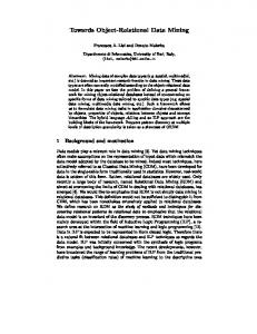
There are many applications that require machines with abilities close to those of human efficiency and consistency in understanding, interpreting and representing the world [1, 2]. Many industries, including agriculture, healthcare, medicine, mining, construction, virtual reality, entertainment, aviation and defence, make use of robots and artificial intelligence. The potential benefits of these technologies have a considerable impact on industry and the community by avoiding dangerous situations for humans by assigning parts of a task to a machine. Such a machine must be able to understand its environment and the semantics of complex objects, considering sub-parts and the functions of objects. The robot may be required to detect the existence of objects, recognise them and avoid or manipulate them. The current research is motivated by urban search and rescue (USAR), where a team of robots is sent to a disaster site. These robots are expected to navigate the site autonomously and, using captured data, find significant features, recognise and classify objects like victims, floors, walls and furniture. The scene might include some data that do not belong to the object of interest (cluttering) or a part of an object surface might be absent due to occlusion [3]. The robots are designed to return a human readable, annotated map [4] showing their findings such as recognised objects [5, 6, 7, 8, 9], and especially, to locate victims and to report their condition [10]. The focus of our research is to use machine learning to build an object classifier for an autonomous robot in an urban search and rescue operation. Time of flight sensors, such as laser range finders, radar and sonar, are often used to obtain 3D data for mobile robotics applications, producing data in the form of a polygonal mesh and point cloud [11, 4, 12]. Therefore, 3D range images, or their corresponding point clouds, which represent a partial view of the environment, are assumed to be the primitive input. 3D depth cameras, such as the Microsoft Xbox Kinect, are now widely used because they provide both range and video images and their cost is much reduced compared with previous generations of similar cameras. In a range image, each pixel’s value represents the distance of the sensor to the surface of an object in a scene from a specific viewpoint [13, 14]. This can be used to infer the shape of the object [15]. The Kinect, also incorporates a colour video camera but in this research, we only use the depth information for object recognition as colour calibration under different lighting conditions is problematic [1]. A range image can be transformed into a set of 3D coordinates for each pixel, producing a point cloud. Figure 1.1 shows a range image of a staircase with four steps, taken by a robot positioned in front of the staircase. In this grey scale image, the darker colour represents closer surfaces. For clarity, a colour-mapped version is also presented. The figure also includes front and top views for the same point cloud. The point cloud has been segmented into planes that are identified by unique colours. A range image only provides a partial view of a scene, since it is taken from one viewpoint. Constructing a complete 3D point cloud for an object requires multiple views. In our early work [16, 17, 18], we extracted planes from the 3D point cloud based on a region growing plane segmentation algorithm [16] and used them as primitives for object categorisation. Planes are useful in built environments, including urban search and rescue 2

Figure 1.1: Range image and its correspondent point cloud (coloured) from front and top view for identifying floors, walls, staircases, ramps and other terrain that the robot is likely to encounter. Modelling a scene from planar patches are used in computer vision, robotics and augmented reality [19]. For example, it has been used for scene understanding [20, 21], localisation [22] and 3D virtual reconstruction of the environment [23]. In this report, we provide details of implementation of the plane segmentation method, feature extraction and configuration for the ILP system used for the learning. Also, we add new features and perform new experiments to evaluate them. In the following sections, we describe the details of segmentation method, the features for extraction, the learning algorithm and the additional experimental results that demonstrate the utility of this approach. We also provide more detail of the system architecture and implementation.

2

The Overall Architecture

The overall system architecture can be decomposed into three general functions: 1. Data gathering: This covers different methods to obtain input images for the system. 2. Pre-processing, feature extraction and labelling: This is mostly performed by the GUI implemented for this research and the configuration files. 3. Learning and evaluation: This is performed outside of the GUI and is controlled by shell scripts that invoke external programs, including ALEPH [24]. Figure 2.1 illustrates the method. Note that there are some alternative labelling scenarios. In one case, the user can label the result of segmentation to form an object. In the second case, it is assumed that the input point cloud includes just one object and all segmented regions form the object. Therefore, automatic labelling is possible if the name of the object for a batch of data is provided. The output of labelling is a set of examples for each object class. For learning and evaluation, the examples are split into training and test sets by using 10-fold cross-validation in our experiments.

The Platform All programs have been implemented on Ubuntu 12.04. For some experiments, we augment the software infrastructure developed by Team CASualty for controlling rescue robots. This has two main components: ‘robotserv’ runs on the robot, performing the time-critical tasks for control and perception. ‘robotgui’ runs on a base station, providing an operator interface and also performs compute-intensive tasks, such as simultaneous localisation and mapping. 3

Fetch & Convert to Point Cloud

Depth images

Pos/Neg Examples

Features

Train/Test split

Training

Test

Rules

Segmentation using normal similarity

No

Labelling?

Yes Features

Do labelling Save as Pos/Neg Examples

Features

Pos/Neg Examples

Performance

(a) Segmentation, Feature Extraction and Labelling

(b) Learning and Evaluation

Figure 2.1: Experimental setup in this research Basestation

Robot

Player

RobotGUI

Drivers Player Player RobotServ

Map Camera Stream

Ice

Snap Sensor Fusion Autonomy

Figure 2.2: An overview of Team CASualty’s platform and its communication channels Both components are configured by an XML file, which specifies which sub-systems are to be used and their settings. Figure 2.2 shows an overview of this platform and its communication channels. We will provide more related details later in Section 8. Next five sections focus on segmentation, feature extraction and representation, the language specification used for learning and new experiments for evaluation. 4

Next item

Fetching data sub-system

calculate normals

remove noise

range image

convert to point cloud

fit planes

planes

another system

Figure 3.1: Illustration of plane segmentation steps and its communication with others

3

Segmentation

We use the plane as the primitive for describing objects, where an object is considered to be composed of a set of planes derived from a point cloud. To find these planes, each point’s normal vector is calculated and used to segment the point cloud. That is, neighbouring points are clustered by the similarity of their normal vectors. A schematic view of the use of plane segmentation is shown as Figure 3.1. Figure 1.1 shows an example of planes found using this method.

3.1

Range Image to Point Cloud

A range image can be transformed into a set of points in 3D space, producing a 3D point cloud [25]. Figure 3.2 shows the corresponding point cloud for Figure 1.1. Because using just one view, such as the front view (Figure 3.2a) is ambiguous, the other views of the same point cloud are also shown. Some points in this point cloud are removed because they are far away, such as the points in the yellow region of the colour-mapped version in Figure 1.1. After this conversion, an ordered (or structured) point cloud is available. Due to the 2D nature of the range image, the neighbourhood of each point in the ordered point cloud can be easily and quickly found. This fact has a great impact on the preprocessing speed. However, it should not be considered a limitation. Many algorithms create a neighbourhood structure when the point cloud is unordered. Therefore, the input is not be limited by range images. Any point cloud representing a partial view of an object can be used similarly. A point cloud can be produced by converting a range image into a set of 3D points. Each pixel in a range image has a 2D coordinate (X,Y) and a depth value, d. The pixels must be projected onto a 3D (X, Y, Z) coordinate system in the robot’s frame of reference. We use a routine provided by Team CASualty [26, 27, 28] in their CASrobot software libraries created for RoboCup Rescue. Lai et al. [29] also provide a MATLAB code1 for the same purpose. 1 http://www.cs.washington.edu/rgbd-dataset/software/depthToCloud.m

5

(a) Front view

(b) Top view

(c) Left view

(d) Right view

Figure 3.2: Corresponding point cloud for range image captured by SwissRanger SR3000 positioned in front of a staircase with four steps (Figure 1.1)

3.2

Plane Segmentation Algorithm

We developed a region growing plane segmentation algorithm in our early work [16] that did not include using a distance threshold. In this report, we update that algorithm and add the distance threshold criterion. The main idea of this region growing algorithm is that neighbouring points with similar normal vector values can form a region and will be represented as a plane. The method starts with a point and traverses the other points through the neighbourhood structure. To decide if the point can be added to the planar surface, it must satisfy the planar surface criteria, given below. We have used the below values for input variables:

min_neighbour_num = 4 base_update_step = 8 num_initial_points = 16 θ = 15◦ − 20◦ The region growing criteria determine when to add a point to a region. Our algorithm is based on using neighbouring points to grow the region. This is where the distance threshold, δ , can be used to decide whether a point is too far away to be accepted as a neighbour for a point. If a point is not too far, it can be included in the not visited neighbours list, candidates, as shown in the algorithm.

6

Algorithm 1 Region growing plane segmentation algorithm using normal vectors Input: PointCloud Input: min_neighbour_num > 0 Input: base_update_step > 0 Input: num_initial_points > 0 Input: min_region_size // minimum region size Input: θ // angle threshold Input: δ // distance threshold Input: angle_m f < 1 // angle modifying factor Input: normal vector f or all points in PointCloud 1: R ← {} // output: Regions 2: for all p in the PointCloud do 3: if p is visited ∨ p is re jected then 4: continue 5: else if number_o f _usable_neighbour(p) < min_neighbour_num then 6: continue 7: end if 8: CR ← p 9: Base_normal ← get_normal_vector(p) 10: candidates ← get_not_visited_neighbours(p, δ ) 11: for all q in candidates do 12: if Size(CR ) < num_initial_points ∨ mod(Size(CR ), base_update_step) = 0 then 13: Base_normal ← get_average_normal_vectors(CR ) 14: end if 15: current_angle ← get_angle(Base_normal, get_normal_vector(q)) 16: accepted ← false 17: if Size(CR ) < num_initial_points then 18: if current_angle < θ then 19: accepted ← true 20: end if 21: else if current_angle < θ ∗ angle_m f then 22: accepted ← true 23: end if 24: if accepted then 25: CR ← CR ∪ q 26: set_visited(q) 27: candidates ← candidates ∪ get_not_visited_neighbours(q, δ ) 28: end if 29: end for 30: if Size(CR ) > min_region_size then 31: set_ f inal_normal_vector(CR ) 32: R ← R ∪CR 33: end if 34: end for 35: return R

7

(a) Colour version, the area having similar normals are highlighted

(b) Normals are represented by RGB colour

Figure 3.3: The top side of box and the ground have similar normal vectors

(a) Colour version; the area having similar normals are highlighted

(b) Normals are represented by RGB colour

Figure 3.4: Another example when part of the two object surfaces have similar normal vectors 3.2.1

Calculating the Distance Threshold

In this section we explain how this threshold can be calculated. Since the segmentation algorithm uses a point’s neighbours for growing the region, there is a chance that a neighbouring point might have a normal vector close to the current point, even though it belongs to another region. This may occur on edges because of the sensor’s point of view as shown in Figures 3.3 and 3.4. For both figures, we have provided a colour version of the scene, highlighting the area which such issue has happened. Also a point cloud version of the scene is provided when the RGB colour of each point is formed by the normal vector of the point. Figure 3.3 shows such situation for a top surface of a box and the ground, while Figure 3.4 illustrates the same for two situations where a side of a box and the wall are having parallel normal vectors and also another wall has parallel normal vector with one side of a wooden stick. A distance threshold may avoid such points, having parallel normals, but are too distant, however, it is difficult to define too far or too distant. Turk and Levoy [30] suggest a method for building a triangular mesh from a range image using a distance threshold. If a point is too far from another point, no edge connects them in the mesh. Range points are flattened by not including depth information, which is using X,Y values and ignoring Z values. Next, the maximum distance between adjacent range points, s, is determined. Finally, the distance threshold, 4s, is defined. The idea is shown in Figure 3.5.

8

Figure 3.5: Illustration of the idea for setting distance threshold to build a mesh from range points [30] Although this thresholding mechanism does not work on our data, the same idea can be applied to another statistical component. We do not flatten the range data, instead, the minimum distance between each point and its adjacent neighbours is calculated. Next, the average of these minimum values, s, is found. Similar to the above method, 4s is used as the distance threshold. Figures 3.6 and 3.7 show some instances of segmentation with and without using distance thresholds. The front view of segmentation with bounding convex hulls and oriented bounding boxes is shown in the first figure. The top surface of one of the boxes is merged with the ground as one planar surface when the distance criterion is not used. Incorporating the distance criterion avoids this problem and better bounding for the related regions can be achieved. A similar situation occurs in Figure 3.7. Here, the front and top views are shown for the convex hull for regions and the oriented bounding boxes from the front view. We compared segmentation, with and without the distance threshold, for 105 images containing stairs. The segmentation of 69 images are improved and become closer to human manual segmentation when employing the distance threshold. 3.2.2

Setting Minimum Region Size

Another parameter is used in this algorithm, that is the minimum region size. If the size of a region, which is the number of points belonging to that region, is less than a threshold, the region is rejected. It is important to set this threshold based on the range camera used for capturing data. For this purpose, a comparable parameter such as camera density is determined, which represents the relative number of pixels due to the camera’s field of view. We defined the camera density for SwissRanger SR3000 as 3.5, while it is 10.0 for Kinect and ASUS Xtion. Using this value, one minimum region size set for the SwissRanger SR3000 can be set for another camera such as the Kinect by using the ratio of their camera densities. Since the fields of view of the available cameras are given to the system, all modules can set these parameters simply by specifying the camera that was used to capture the image. Another factor to be considered is the sampling rate used to reduce the number of points in the point cloud for faster processing.

9

(a) Colour version of the scene

(b) Front view, bounding convex hull, without and with using distance threshold

(c) Front view, oriented bounding box, without and with using distance threshold

Figure 3.6: Boxes in a scene, the effect of using distance threshold To calculate an appropriate minimum region size, we use min_region_size_base as the base number of points for a range image taken by SwissRanger SR3000. This number is scaled down in respect to the sub-sampling rate used. This threshold is also scaled by the corresponding camera density. For example, we used 175 as the base value for planar objects in various experiments.

4

Feature Extraction

We have used the plane as the primitives for describing objects, where an object is considered to be composed of a set of these primitives derived from a point cloud. The point cloud is represented by a set of features extracted from these regions and by relationships between regions. These features and relations include: the attributes of each individual region, the relationships between every pair of regions, and features based on an aggregation of the regions. After extracting these features, sets of regions are labelled according to the class to which they belong. The ALEPH ILP system [24] is used to build a classifier for each class, where objects belonging to that class are considered positive examples and all other objects are treated as negative examples. 10

(a) Colour version of the scene

(b) Front view, bounding convex hull, without and with using distance threshold

(c) Top view, bounding convex hull, without and with using distance threshold

(d) Front view, oriented bounding box, without and with using distance threshold

Figure 3.7: Bookcase in a scene, the effect of using distance threshold

11

(a) Diameter

(b) Width

Figure 4.1: Features of a convex hull

4.1

Single Region Features

4.1.1

Normal Vector:

The mass and normal vector of a planar region are the average of the points belonging to the plane and the average of their normal vectors, respectively. The normal vector is represented by its spherical coordinates (θ and φ ) [31], where θ is defined as zero when x=y=0. The normal vector is normalised, so ρ = 1 for all cases. 4.1.2

Region Boundary

The boundary of a planar region can be represented by a convex hull [32]. For example, Tsai et al. [33] used convex hulls to form boundaries of planes. There are many convex hull algorithms [34, 35, 36, 37]. The method employed in this research is a modification of the Andrew’s algorithm [38]. From the convex hull, two more features can be extracted: the diameter of the convex hull and the width of the convex hull. The former is the distance between two points on the convex hull that are furthest away [39]. The latter can be defined as the distance between two parallel lines containing the convex hull [40]. The width and diameter for a convex hull are illustrated in Figure 4.1. Calculating the ratio between these two features, another scale-invariant feature, convex_ratio, can be created. Some algorithms [40, 41, 39] are described for finding the diameter and width of a convex hull. We use the source code2 provided by Schneider and Eberly [42] that implements rotating calipers [41]. Since we are using range data and the point cloud does not show the whole 3D object shape, it is sufficient to find a 2D convex hull. The 2D convex hull algorithm introduced by Andrew [38] serves as a starting point. To fit a convex hull around a region, its points must be projected onto a 2D space. This is performed by projecting the region onto the smallest dimension of its oriented bounding box. After fitting the convex hull, it is projected back to 3D coordinates. 4.1.3

Bounding Box and Region Distribution

An additional feature is how a region is distributed. One way to calculate this is by using the bounding box and calculating the length of its three axes. By determining the difference between the maximum and minimum values of a region’s point coordinates (4x, 4y and 4z) and comparing them, we decide along which axis the plane is distributed the most. 2 http://www.geometrictools.com/LibMathematics/Containment/Wm5ContMinBox2.cpp

12

Another feature set consists of the ratios between each pair of the above values ( 4x 4y , 4x 4z ),

4y 4z

and

which is robust to scaling. These attributes are in the sensor’s frame of reference and

since they are not object-centred, rotating the object might affect them. 4.1.4

Oriented Bounding Box

Since region distribution does not consider orientation, it is useful to create an oriented bounding box for each region and to use its properties in the object description. To fit an oriented bounding box to each region, we use the method presented by Gottschalk [43] and implemented by Gregson [44]. Similar to 4x, 4y and 4z, three values 4di can be determined, which show how the region is distributed along the oriented bounding box axes (where 4d1 ≥ 4d2 ≥ 4d3 ). However, of interest are the ratios

4d1 4d2 4d2 , 4d3

and

4d1 4d3 .

Since the oriented bounding box

is robust to rotation, these ratios benefit from this robustness in addition to their scaleinvariance. Figure 4.2 shows the RGB-colour version of the scene, bounding boxes and oriented bounding boxes after the planar segmentation. Each region is represented by a different colour using the provided colour legend. In contrast to bounding boxes that are not object centred, oriented bounding boxes are object centred and can provide features that are invariant to transformation such as rotation. Since oriented bounding boxes were a later addition to our research, both feature sets are used separately in various experiments. Thus, bounding box features are introduced first, and are later replaced by oriented bounding boxes.

4.2

Region Relationships

The relationships between shape primitives describe the structure of an object and can be used to find similarities between instances of object classes. Thus, after finding segments and calculating their individual properties, relationships are constructed between each pair of primitives. These are in the form of how the regions are located with respect to each other and how their individual features can be compared. 4.2.1

Angle Between Two Regions

The angle between two regions is the angle between their normal vectors. 4.2.2

3D Spatial Relationship

Another relationship is based on binary topological [45] and spatial [46, 47] relationships such as the directional relationship [48, 49] that describes how two planes are located with respect to each other. For example, as shown in Figure 4.3, rectangle b is located on the east side of rectangle a, from the perspective of one 2D view. To find this direction between two rectangles, the line that connects both centres is used. The line that connects the centres of a and b is closer to the east axis defined on the centre of rectangle a. Thus, we say that b is east of a. This definition can be easily extended to other directions, north-east, north-west, south-west and south-east. Note that this relation is view dependent. 13

(a) Colour legend

(b) Pitch/roll ramp

(c) Stairs

(d) Stairs

(e) Kinect box on the table

Figure 4.2: RGB-colour image (left), bounding boxes (middle) and oriented bounding boxes (right) for some selected objects. Each region is represented by a different colour using the provided colour legend.

14

Figure 4.3: Example of spatial arrangement for four rectangles a, b, c and d A further relationship is when two rectangles share partial edges or one rectangle covers the other. In this figure, rectangle a covers c, while rectangles b and c are connected. Also rectangle d covers all rectangles a, b and c. This concept is defined for 2D space and requires some modification to be used for 3D space. Several researches have studied this kind of relationship. Borrmann et al. [50] define 3D spatial data types and their operators and devise a spatial query language. Berretti and Del Bimbo [51] propose a modelling technique for 3D spatial relationship, while Zlatanova et al. [52] give an overview of models for 3D topology. Ellul and Haklay [53] identify the requirements for 3D spatial relationships and Chen and Schneider [54] discuss this 2D to 3D generalisation and propose a neighbourhood configuration model to encode the topological relationship. We chose to test a simpler approach in this research. In Figure 1.1, two views of the same segmented 3D point cloud are shown: front view and top view. Both views are shown as 2D images. Regions that might not look parallel to each other from one view, are clearly parallel from another. The 3D view can be projected onto two 2D views to find the spatial-directional relationships in each 2D view. For this purpose, a bounding cube, with respect to the sensor’s coordinate frame, is generated for each set of points assigned to a region. Two projections of this cube are then used to represent the minimum bounding rectangles for the region from each of the two views. The projections are on the XY plane (front view) and the ZX plane (top view). Referring to Figure 4.3, the X-axis represents the West to East and the Y-axis shows the South to North direction in the front view. For the top view, the X-axis is in the South to North direction while the Z-axis represents the West to East direction It is possible that redundant relations will be generated for an object description. However, there are mechanisms for eliminating redundancies. For example, if the bounding rectangle of region X from a particular view is covered by the bounding rectangle of region Y, and region Z has another relationship with region Y, the relationship between region Z and X in that view is eliminated. This can be seen in the front view of Regions 1, 4 and 5 in Figure 4.2e. Region 5 is covered by Region 4, while there is another relationship between Regions 1 and 4. As a result, since the coverage relationship between Regions 4 and 5 dominates any possible relationship between Regions 1 and 5, the relationship between Region 1 and Region 5 is eliminated.

15

u = ns

(pt −ps ) v = u × kp t −ps k2

α = v.nt

w = u×v

s) φ = u. (pt −p d

θ = arctan(w.nt , u.nt ) d =k pt − ps k2 Figure 4.4: Relative difference between two masses and their associated normals [57] 4.2.3

Relative Difference Between Normal Vectors

Another region relationship is calculated from the difference between two centres of mass (ps and pt ) that belong to two regions, using their associated normal vectors (ns and nt ). This feature is used in the PCL [55] for creating Point Feature Histograms (PFH) [56]. The relationship is defined by a 4-tuple < α, φ , θ , d > and a coordinate frame at ps as shown in Figure 4.4, where d is the Euclidean distance between two points.

4.3

Region-Set Features

Another category of features considers all regions that together form an object. For example, the pitch/roll ramp is formed by Regions 2 and 3 in Figure 4.2b, while Regions 2, 3 and 5 in Figure 4.2e form the box. In the case of the stairs in Figures 4.2c and 4.2d, the number of regions that make up the object class is not fixed as stairs may have a different number of steps. For example, region-sets (1,3,4,5,6) and (1,3,4,5) in Figure 4.2c form stairs. This can be handled by a recursive class description. 4.3.1

Number of Regions Forming an Object

Following the previous point, many objects will have a fixed number of regions visible in a particular view, therefore, the number of visible regions may be used as a feature. However, as noted above, in some cases that number is not always useful. 4.3.2

Oriented Bounding Box and Corresponding Ratios

Another feature can be calculated by making an oriented bounding box for the whole object. Similar to the single region feature, three ratios for each box are extracted.The third category of features is based on considering all regions that form an object.

Binning for Angle and Ratio values We have used a binning system instead of using the exact value for angles and ratios. An angle will be represented by one of the following bins as 0±15, 45±15, 90±15, 135±15, 180±15, 22.5±15, 67.5±15, 112.5±15 and 157.5±15 or their negative corresponding.

16

Similar to binning used for angle values, ratios are binned in intervals defined around fixed values 1, 1.5, 2, 2.5, ... with the interval length 0.5 (i.e. ±0.25). That is, they can be represented as: { i ± 0.25; i = 1, 1.5, 2, 2.5, 3, ...} This binning system works for ratios ≥ 1 such as OBB ratios

4d1 4d2 4d2 , 4d3

and

4d1 4d3

which

are always ≥ 1. When the ratio 1, and to avoid having small ratios such as 0.005, the concept of inverted ratio values is defined here. The inverted ratio can be explained by an example. If a b then b a

≥ 1. Instead of using the ratio

a b

1, we use

b a

a b

1, and therefore

≥ 1. To show that we have applied this

inversion, we represent the inverted ratios by a negative sign. For example, when its inverted ratio is

b a

a b

= 0.78,

= 1.28. This value (1.28) must be represented as 1.5±0.25, however

since it is an inverted version, its corresponding ratio bin will be represented as -1.5±0.25.

5

Feature Representation

The directional relationships of rectangles shown in Figure 4.3, can be expressed easily as Prolog facts. For example, the Prolog facts for some of the directional relationships in Figure 4.3 are:

east(a,b). /* (rectangle) a is on the east side of b. */ covers(a,c), not_covers(a,b). /* a covers c and a does not cover b. */ connected(b,c). /* b is connected to c. */ covers(d,X). /* d covers all rectangles. */

Here, the names of the relations are east, covers, not_covers and connected. The last clause, is not a ground fact. It is a generalisation that contains the variable X, and subsumes the three ground facts:

covers(d,a). covers(d,c). covers(d,b). This section, explains how features and relations are encoded as Prolog facts. To represent a region-set that includes one or more regions, a Prolog list is used. The type of each region is represented by a particular primitive. For example, when only plane segmentation is applied, each region is a plane. However, if the segmentation algorithm can provide more primitives such as a cylinder, then the relation name used in Prolog will show the corresponding type. It is important that each region is denoted by a unique name or ID. As shown, there are five planar regions as the result of segmentation in Figure 4.2e. The regions shown in this figure can be represented as below, which is automatically generated as the result of segmentation. The general form is:

plane(plane_ID). 17

and the instances of planes are:

plane(pl_001). plane(pl_002). plane(pl_003). plane(pl_004). plane(pl_005). Since Regions 2, 3 and 5 form a box, this combination can be represented as below, which can be created automatically as the result of supervised training or labelling, as discussed later. There are two ways to represent a region-set belonging to a class: using the name of the class as the relation name, or using the class name as an argument. That is, the general form can be either:

object_class_name(region_set). % or class(object_class_name, region_set). and in this example it will be

box([ pl_002, pl_003, pl_005 ]). % or class(box,[ pl_002, pl_003, pl_005 ]). There is no significant difference between these two representations. Since we construct a binary classifier for each class, it is preferable to use the same declarations and settings for each class without changing the names of the relations. The first representation requires unique declarations and settings for each class, but is easier to read. Therefore, we use the second representation in our implementation, to save some effort, but in our explanations, we sometimes use the first notation, for clarity. As mentioned earlier, the features are grouped into three categories: single region features, region relations and region-set features. The next section describes the representation of these features as defined for learning.

6

ALEPH and Language Specification for Learning

ALEPH is the machine learning toolkit that is mainly used in this research. A part of the result of learning the class stairs using ALEPH is shown below. The features and relations for a large set of images are extracted and passed to ALEPH as background knowledge. The implemented GUI is used to label 237 instances as positive examples and 656 negative examples of the object stairs. It is also necessary to give some constraints to ALEPH to reduce the search for the hypothesis. One of the rules constructed by ALEPH is given below. In this example, plane segmentation is used and ALEPH is compiled with SWI-Prolog.

18

%[Rule] [Pos cover = 213 Neg cover = 0] stairs(REG_SET) :member(C, REG_SET), member(D, REG_SET), angle(D, C, `0 ± 15'), member(E, REG_SET), angle(E, C, `90 ± 15'), angle(E, D, `90 ± 15'), distributed_along(E, axis_X). This rule covers 213 positive examples (over 89.87% of total positives) and no negative examples. The member relation, which is predefined in Prolog, specifies that the first argument is a member of the list that is provided as the second argument. In other words, the primitive (plane) exists in the given region-set or the region belongs to the region-set. This clause defines a region-set as belonging to the class stairs if it has at least three planes, C, D and E of which regions C and D are approximately parallel, both regions C and D are approximately perpendicular to region E and region E is distributed mostly along the X-axis. In addition to providing positive and negative examples to ALEPH, some constraints on the hypothesis language must be given [24]. Mode declarations have the form:

mode(RecallNumber,PredicateMode). The first argument, recall number, specifies the maximum number of instances for the predicate. This must be a positive number greater than or equal to 1 or ‘*’, which represents no limit. For example, for predicate parent(P, C), the recall number is 2 since a child can have two parents [58], while for sister(S1, S2), the recall number does not have a limit. The second argument defines how a predicate must be called. It follows the template below:

p(ModeType, ModeType, ...). ModeTypes can be simple or structured. A simple ModeType has three possible forms: +T, -T and #T. A ‘+’ means that the variable is treated as input of the specified type, while ‘-’ indicates an output variable of the given type and ‘#’ specifies that it is a constant of the given type. A structured ModeType follows the form f(..) where f is a function symbol, and its arguments may also be simple or structured ModeTypes. For example,

:- mode(1,mem(+number,+list)). shows a mode declaration having solely simple modetypes while

:- mode(1,mem(+number,[+number|+list])). shows an example having both. Determination statements specify the predicates that might be used for hypothesis construction:

19

:::::::::::::::::::::-

modeb(1,angle(+region,+region,#angle_bin)). modeb(1,normal_spherical_theta(+region,#angle_bin)). modeb(1,normal_spherical_phi(+region,#angle_bin)). modeb(*,ratio_yz(+region,#ratio_bin)). modeb(*,ratio_xz(+region,#ratio_bin)). modeb(*,ratio_xy(+region,#ratio_bin)). modeb(*,ch_ratio(+region,#ratio_bin)). modeb(*,dr_xy(+region,+region,#direction)). modeb(*,dr_xz(+region,+region,#direction)). modeb(*,distributed_along(+region,#axis)). modeb(*,obb_ratio23(+region,#ratio_bin)). modeb(*,obb_ratio13(+region,#ratio_bin)). modeb(*,obb_ratio12(+region,#ratio_bin)). modeb(1,rel_dif_nv_alpha(+region,+region,#angle_bin)). modeb(1,rel_dif_nv_phi(+region,+region,#angle_bin)). modeb(1,rel_dif_nv_theta(+region,+region,#angle_bin)). modeb(1,rs_obb_ratio23(+region_set,#ratio_bin)). modeb(1,rs_obb_ratio13(+region_set,#ratio_bin)). modeb(1,rs_obb_ratio12(+region_set,#ratio_bin)). commutative(angle/3). commutative(rel_dif_nv_alpha/3).

Figure 6.1: Mode declarations corresponding to the features used in this research

determination(TargetName/Arity,BackgroundName/Arity). The first argument specifies the name and arity of the target predicate, which appears in the head of the hypothesis clauses. The next argument defines name and arity of a predicate which can contribute in the body of such clauses. Only one target predicate can be used. The features were discussed in previous sections. Next, we introduce a specification that can be used to guide our object classification method using ALEPH. Each region-set includes some regions and each region has some attributes. In addition, each region pair and each region-set might have some relations. Therefore, the following are declared:

:- modeb(*,n_of_parts(+region_set,#n)). which directs the learning algorithm to consider the number of regions in the region-set.

:- modeb(*,member(-region,+region_set)). which selects each region in the region-set for further processing. Other features can be declared as Figure 6.1, where the relations angle and rel_dif_nv_alpha are commutative. For the hypothesis mode declaration, there are two possible approaches, as discussed in Section 5: • Defining a different mode for each object class:

:- modeh(*,box(+region_set)). :- modeh(*,stairs(+region_set)). 20

%... :- modeh(*,wall(+region_set)). • Defining a single mode with the class name as an argument:

:- modeh(*,class(#class_name,+region_set)). class_name(box). class_name(stairs). %... class_name(wall). Similar to the previous example, an appropriate determination must be provided based on the above modes:

:- determination(box/1,angle/3). % for each object class and when using the second approach for hypothesis mode declaration:

:- determination(class/2,angle/3). Some constant definitions are also required as below:

%--- Axes --axis(axis_X). axis(axis_Y). axis(axis_Z). %--- directions --direction(north). direction(east). direction(south). direction(west). direction(is_covered). direction(covers). direction(connected). %--- angle_bins --anglebin(`0 ± 15'). anglebin(`-0 ± 15'). %... anglebin(`180 ± 15'). anglebin(`-180 ± 15'). anglebin(`22.5 ± 15'). anglebin(`-22.5 ± 15'). %... anglebin(`157.5 ± 15'). anglebin(`-157.5 ± 15'). %--- ratio_bins --ratiobin(`1.0 ± 0.25'). ratiobin(`-1.0 ± 0.25'). ratiobin(`1.5 ± 0.25'). ratiobin(`-1.5 ± 0.25'). %... ratiobin(`10.0 ± 0.25'). ratiobin(`-10.0 ± 0.25'). ratiobin(`10.5 ± 0.25'). ratiobin(`-10.5 ± 0.25'). 21

Parameter Settings in ALEPH Some parameter settings used in ALEPH [24] are required: • The number of literals for an acceptable clause can be limited using the following the parameter setting. The default value is 4. It is set to a higher value, 10.

:- set(clauselength,+V). • As the dataset contains noise, experiments vary ALEPH’s tolerance to noise using the following directive. The default value for V is 0, i.e. no noise.

:- set(noise,+V). • Another parameter is an upper bound for the number of nodes for exploration during the search. The default value is 5000. A higher value of 10000 is used here and can be set by:

:- set(nodes,+V). • Each clause covers some positive examples. However, it is possible to specify the minimum number to reject clauses with a small coverage. The default value is 1.

:- set(minpos,+V).

7 7.1

Additional Experimental Evaluation Feature evaluation

An RGB-D dataset of some common household objects is provided by Lai et al. [29] using a Microsoft Xbox Kinect sensor. Only one object on a turntable appears in each scene. As a result, after applying segmentation to the input scene, there is no need to select which regions form an object, since most regions participate. We have performed some experiments using this dataset in our previous work [18]. Although the dataset includes 51 classes, only a subset has been chosen, including ball, bowl, cap, cereal box and coffee mug. Note that each class has a different number of physically distinct instance sets. A physically distinct instance set (PDIS) is a collection of images of a particular instance of a class taken from different angles by rotating the object on a turntable and from different camera mounting points. Using the original captured and cropped images, sub-samples are taken from each sequence for each object, taking every ith frame. There is a specific split arrangement for training/testing data. Data for each object class come from a different physically distinct instance each of which is stored separately. For example, data for the class ball are saved in 7 folders, while the number of folders for the bowl object class is 6. As suggested by Bo et al. [59], for each iteration of learning, one PDIS of each object is chosen randomly as the test set and the rest form the training set. This random train/test split technique is k-fold cross validation, with a specific implementation to test the classification on a PDIS of an object which has not been used for training. 22

Table 7.1: Numerical information about the chosen subset of RGB-D dataset used as the first dataset Object class

Pos#

Neg#

PDIS#

Number of images for each PDIS

ball

225

582

7

[33,32,33,32,32,32,31]

bowl

160

647

6

[24,24,24,23,33,32]

cap

104

703

4

[26,27,25,26]

cereal box

119

688

5

[23,25,25,24,22]

coffee mug

199

608

8

[22,23,23,22,22,22,33,32]

Total

807

PDIS#: Number of physically distinct instance sets

We refer to this implementation as folder-based split. For each class, the chosen physically distinct instance sets for training are treated as positive or negative examples for training based on the current object, while the union of test sets is used for testing for all objects. In this section, experiments are conducted on a subset of this RGB-D dataset with different configurations. The aim is to measure learning performance using only plane segmentation on household objects that have curved surfaces. The distance threshold option is used. The experiments seek to test some features not covered in the previous experiments: • Region-set oriented bounding box and its ratios (Section 4.3.2). This feature is added to set to the basic configuration to determine how it affects the performance. • Relative difference between normals (Section 4.2.3) instead of directional relationship features. • Using each region’s oriented bounding box features (Section 4.1.4) instead of its bounding box features. • Combine two of the above new features. The configurations for this set of experiments are presented as in Figure 7.1. There are five configurations using five classes from the RGB-D dataset based on a sub-sampling factor of 25. Since the objects in the RGB-D dataset are much smaller when compared to the planar objects previously used, the minimum size for a region to be accepted is decreased by setting min_region_size_base=10. The number of physically distinct instance sets for each class, the number of images in each PDIS and the number of positive and negative examples used for this experiment set are presented in Table 7.1. As mentioned earlier, the folder-based split approach is used for this experiment set. Table 7.2 shows the performance comparison for the configurations used including the number of rules and the compression average. The measures are provided per configuration in the form of the weighted mean and standard deviation values. The results show that:

23

% method: PLOCRL (PLane-based Object Categorisation using Relational Learning) % segmentation method used: just plane segmentation

% minimum region size: decreased. % angle threshold: 20◦ % distance threshold: used :- set(noise,10). % data: RGB-D dataset using every 25th frame % ball, bowl, cap, cereal box, coffee mug % features common between all configurations % angle % normal_spherical_theta, normal_spherical_phi % ch_ratio % additional features for configuration(1) % ratio_yz, ratio_xz, ratio_xy, distributed_along % dr_xy, dr_xz % additional features for configuration(2) % % % %

ratio_yz, ratio_xz, ratio_xy, distributed_along dr_xy, dr_xz rs_ratio_obb23, rs_ratio_obb13 rs_ratio_obb12

% additional features for configuration(3), (testing dr versus rel_dif_nv) % % % %

ratio_yz, ratio_xz, ratio_xy, distributed_along rel_dif_nv_alpha rel_dif_nv_phi rel_dif_nv_theta

% additional features for configuration(4), (testing BB versus OBB) % % % %

obb_ratio23 obb_ratio13 obb_ratio12 dr_xy, dr_xz

% additional features for configuration(5), (using both OBB and rel_dif_nv) % % % % % %

obb_ratio23 obb_ratio13 obb_ratio12 rel_dif_nv_alpha rel_dif_nv_phi rel_dif_nv_theta

Figure 7.1: Configurations for experiments involving the RGB-D dataset 24

Table 7.2: Comparing overall weighted mean and the standard deviation for feature evaluation experiments Experiment

Accuracy (%)

Precision (%)

Recall (%)

Number of

Compression

Rules

Average

1

89.21±2.88

70.47±4.24

76.97±7.82

11.79±0.78

16.44±1.50

2

88.71±2.91

68.64±5.21

76.66±6.47

12.96±1.18

15.17±1.30

3

89.29±2.99

69.97±5.60

77.26±7.69

11.99±0.40

15.45±1.45

4

87.79±2.55

67.43±3.82

74.67±7.26

11.12±0.65

15.38±1.06

5

90.84±2.25

73.52±3.06

81.92±7.96

10.13±0.62

19.65±2.05

Experiment 1 :

No feature substitution

Experiment 2 :

Adding oriented bounding box ratios for region-set

Experiment 3 :

Directional relationships versus relative difference between normals

Experiment 4 :

Bounding Box versus Oriented Bounding Box for each region

Experiment 5 :

Combination of 3 & 4

• Using the region-set oriented bounding box feature has no major effect on overall measures at least for the selected object classes. • The alternative features (using relative difference between normals instead of directional relationships and the region’s oriented bounding box instead of bounding box) are practical and even their substitution combination increases the performance and average compression, as well as reducing the number of rules. In addition to the overall measures, it is useful to examine the performance measures per class as shown in Table 7.3. The results show that: • Accuracy, precision and recall are improved after each single substitution (Configurations 3 and 4) more than 40% of the time. • Comparing the basic configuration (configuration 1) and combined substitution configuration (configuration 5), the accuracy, precision and recall are improved 80%, 60% and 80% of the time respectively, which suggests the benefits of using these substitutions together. • Accuracy, precision and recall are improved for the class cap after using the region-set bounding box ratio feature, which shows its potential for further investigation. Regarding the number of rules and compression average: • Improvement is obtained more than 60% of the time by any single feature substitution. • Comparing the basic configuration (configuration 1) and combined substitution configuration (configuration 5), 80% of the combined substitutions have fewer rules with a greater compression average. 25

Table 7.3: Comparing each object class weighted mean and the standard deviation for feature evaluation experiments Object

ball

bowl

cap

cereal box

coffee mug

Experiment

Accuracy (%)

Precision (%)

Recall (%)

Number of

Compression

Rules

Average

1

88.39±3.16

73.65±9.64

85.27±10.53

11.89±1.50

26.55±2.78

2

88.39±3.16

72.87±6.85

84.87±10.48

12.22±2.23

26.91±3.96

3

87.27±2.82

70.64±6.63

82.04±6.55

13.44±1.97

21.38±3.43

4

85.03±2.23

66.15±6.32

79.7±11.44

11.11±2.17

24.55±3.97

5

87.42±2.64

69.13±6.16

87.35±7.81

10.56±1.40

29.2±1.93

1

85.32±4.24

65.33±11.61

62.62±25.15

11.67±1.89

12.38±1.61

2

84.13±3.31

59.86±12.72

63.09±30.56

11.89±2.59

11.58±1.80

3

84.58±4.79

62.62±11.95

60.53±29.29

11.44±1.61

14.41±3.16

4

82.7±5.29

56.37±12.56

57.19±26.07

10.33±1.79

12.47±2.88

5

85.55±4.12

63.6±8.06

65.39±27.49

10.89±2.04

12.47±2.10

1

88.02±3.31

69.47±8.83

70.13±11.22

6.89±0.96

12.44±2.02

2

88.62±3.31

71.96±8.60

70.74±10.39

10.00±1.41

7.69±2.09

3

88.02±2.82

70.09±8.60

70.31±7.87

7.56±1.39

8.69±1.72

4

89.14±4.24

73.15±12.04

69.66±15.19

6.11±1.26

12.85±3.10

5

94.9±2.44

86.71±9.05

88.85±4.12

6.11±1.17

19.17±4.38

1

97.38±1.73

91.9±8.12

94.09±7.07

3.44±0.48

35.8±5.09

2

96.55±2.23

88.73±9.00

93.33±6.40

3.78±0.65

35.24±5.67

3

96.78±1.73

89.41±6.78

93.31±6.16

4±0.82

31.49±4.21

4

97.67±1.41

93.2±5.74

94.06±9.11

3.11±0.85

40.93±10.08

5

97.67±1.41

93.5±3.74

93.26±8.94

3.78±0.8

34.24±7.33

1

78.44±4.58

45.44±8.94

65.16±13.96

17.44±3.03

8.42±1.68

2

77.47±4.79

43.83±8.42

64.24±11.31

18.56±3.34

8.1±1.14

3

81.06±5.19

49.96±8.71

72.42±15.96

15.78±2.68

8.78±2.75

4

75.82±3.31

41.44±7.48

64.92±5.74

17.78±2.90

6.47±1.11

5

79.86±3.00

47.65±6.48

66.9±18.22

12.78±2.68

11.32±2.28

Experiment 1 :

No feature substitution

Experiment 2 :

Adding oriented bounding box ratios for region-set

Experiment 3 :

Directional relationships versus relative difference between normals

Experiment 4 :

Bounding Box versus Oriented Bounding Box for each region

Experiment 5 :

Combination of 3 & 4

26

(b) Bowl

(a) Ball

(c) Cap

(d) Cereal box

(e) Coffee mug

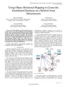
Figure 7.2: Colour and segmented version of selected objects from the RGB-D dataset Because only plane primitives have been used, lower accuracy might be expected for this experiment in comparison to previous experiments in which objects with mostly planar surfaces were used [16, 17, 18]. However, the high accuracy obtained in the above experiments shows that the method can be applied to an object with curved surfaces. However, rules are expected to be larger, with less compression. Thus, extending segmentation to cover more primitive shapes such as cylinders and spheres might lead to an improvement in accuracy, but particularly should result in rules that are more readable and may be learned more quickly. More regions should be expected when using only plane segmentation. Figure 7.2 shows an example for each class after segmentation in which each region is represented by its convex hull. Extending the segmentation should decrease the number of extracted regions as well as leading to less complexity for learning.

7.2

Comparison with a Non-Relational Object Classifier

As discussed in our previous work [18], Bo et al. [59] present a non-relational object classifier using an RGB-D dataset [29] with promising accuracy. Their method is compared with the method developed in this research, PLOCRL, using folder-based split approach as previously described. Bo et al. [59] provide MATLAB code3 for comparison. However, at the time of this experiment, a modification of the classification method was needed following the documentation provided in their C++ code, which meant using the ‘linear’ option to scale the training and testing data. They introduced depth kernel descriptors for classification using depth and colour images. However, since the current research uses solely range data, and their corresponding point clouds, the related gradient kernel descriptors (Gradient KDES), local binary pattern kernel descriptors (LBP KDES), dense normal kernel descriptors (Normal KDES), size kernel descriptors (Size KDES), and their combinations are used for comparison. 3 http://www.cs.washington.edu/ai/Mobile_Robotics/projects/kdes/

27

Table 7.4: Numerical information about the chosen subset of RGB-D dataset used as the second dataset Object class

Pos#

Neg#

PDIS#

Number of images for each PDIS

ball

225

761

7

[33,32,33,32,32,32,31]

bowl

160

826

6

[24,24,24,23,33,32]

cap

104

882

4

[26,27,25,26]

cereal box

119

867

5

[23,25,25,24,22]

coffee mug

199

787

8

[22,23,23,22,22,22,33,32]

sponge (planar)

179

807

6

[26,24,32,33,31,33]

Total

986

PDIS#: Number of physically distinct instance sets Table 7.5: Numerical information about the chosen subset of RGB-D dataset used as the third dataset Object class

Pos#

Neg#

PDIS#

Number of images for each PDIS

ball

225

889

7

[33,32,33,32,32,32,31]

bowl

160

954

6

[24,24,24,23,33,32]

cap

104

1010

4

[26,27,25,26]

cereal box

119

995

5

[23,25,25,24,22]

coffee mug

199

915

8

[22,23,23,22,22,22,33,32]

sponge (total)

307

807

10

[26,24,32,33,31,33,32,32,32,32]

Total

1114

PDIS#: Number of physically distinct instance sets

Three datasets are used for this comparison. One dataset includes five classes used in the previous section (ball, bowl, cap, cereal box, coffee mug) taking every 25th image from the image sequence as shown in Table 7.1. For the second dataset, a subset of the class sponge is added, which is mostly planar with the same sampling factor (see Table 7.4). The third dataset is the second dataset plus the rest of the class sponge, which is not mostly planar with the same sampling factor (Table 7.5). The PLOCRL method uses two configurations: basic and extended, which are the first and the last configurations (configurations 1 and 5 respectively) explained in the previous section, as before and after both feature substitutions. For both configurations, only plane segmentation is used. Since Bo et al. [59] give only the average accuracy of classification, this measure is used with the above descriptors to compare against this research’s method, PLOCRL, for these two configurations. The results are shown in Table 7.6. Bo et al. [59] build a multi-class classifier, while the method developed here employs a binary classifier for each object class. Therefore, the accuracy measure for our method must consider positive examples for each class, ignoring negative examples as discussed 28

Table 7.6: Comparing mean and the standard deviation of accuracy with a non-relational method using three subsets of the RGB-D dataset Dataset 1

Dataset 2

Dataset 3

Accuracy

Accuracy

Accuracy

Gradient KDES

69.38±8.56

69.38±8.56

69.87±14.69

LBP KDES

65.86±14.31

68.95±8.65

71.73±13.44

Normal KDES

77.25±7.31

72.02±8.06

72.76±12.24

Size KDES

74.61±12.83

68.32±13.11

76.05±9.47

Gradient + LBP KDES

82.53±9.60

74.08±12.62

78.98±11.60

combination of all

84.36±8.63

76.79±13.28

82.03±10.15

Basic version of PLOCRL

75.23±8.30

76.85±5.10

73.26±4.38

Extended version of PLOCRL

79.92±8.16

79.70±6.05

74.27±8.18

Method

Dataset 1:

ball, bowl, cap, cereal box, coffee mug

Dataset 2:

ball, bowl, cap, cereal box, coffee mug, sponge (planar)

Dataset 3:

ball, bowl, cap, cereal box, coffee mug, sponge (total)

by Abudawood and Flach [60]. That is, we calculate and sum true positive values for all classes, then divide the result by the total number of positive examples used for testing to determine the accuracy of PLOCRL as a multi-class classifier. In this case, since positive examples of one class are treated as negative examples of other classes, when TPi represents the true positive for the binary classifier for object class i, then the accuracy for the multiclass classifier using n binary classifiers is

n

n

∑ T Pi

∑ T Pi

i=1 n

n

∑ T Pi + ∑ FNi i=1

, which is equal to

i=1

N

, where N

i=1

is the total positive examples used for testing. Although the PLOCRL method used solely planar primitives, the comparison shows that its accuracy is very close to a state-of-the-art classifier even when it is tested on a subset of common objects having curved surfaces. The PLOCRL outperforms the majority of depth kernels most of the time. While the accuracy of a non-relational object classifier decreases by adding a planar shape object to the dataset, the accuracy of PLOCRL method increases. However, as expected, due to using plane segmentation, adding non-planar object shapes affects the accuracy of the method slightly. Besides accuracy, the method inherits relational learning benefits over non-relational methods. It describes the relationship between subparts, which is a useful feature of relational learning. In addition, knowledge accumulation, learning by using previously learned concepts in background knowledge, is an additional superior aspect of using relational learning. These two properties are not present in other methods such as the depth kernel descriptors.

29

7.3

Discriminative versus Descriptive Rules

The rules induced by ALEPH are discriminative rather than descriptive. For example, a stairs object can be defined by a different number of regions:

stairs([pl_01,pl_03,pl_04,pl_05,pl_06,pl_08]). stairs([pl_01,pl_03,pl_04,pl_05]). Both form a staircase but one is a subset of the other. If the induced rule for the smaller region-set can cover the larger one, ALEPH will not generalise it. That is, ALEPH creates a rule that is sufficiently practical to discriminate, but it is not necessarily the most descriptive rule. To create a more descriptive rule, further directions must be given to ALEPH. Additional analysis of examples used for training may also be necessary. Searching for clauses in ALEPH is affected by two parameters: the search strategy and the evaluation function. These parameters can be defined by:

:- set(search,Strategy). :- set(evalfn,Evalfn). where Strategy can be ar, bf, df, heuristic, ibs, ic, id, ils, rls, scs and false. For example, bf, which is the default strategy, enumerates shorter clauses before longer ones. EvalFn can take the values coverage, compression, posonly, pbayes, accuracy, laplace, auto_m, mestimate, entropy, gini, sd, wracc, or user define. Investigating the options for the search strategy and the evaluation function may be helpful to achieve rules that are more descriptive. As shown earlier in the previous work [17, 18], learned concept descriptions can be put into background knowledge to help learn another concept description. Additionally, a concept like stairs can be represented by a recursive description. To achieve a recursive rule, it might be necessary to define an evaluation function that rewards a recursive rule, since a recursive rule might be ignored if another rule is considered superior with respect to the current evaluation function. However, the most important factor in achieving a recursive rule is providing appropriate mode declarations and determinations which guide ALEPH to reduce the size of input arguments in the hypothesis. ALEPH constructs three non-recursive rules for stairs, using only angle predicates as shown in Figure 7.3. It is also able to construct recursive rules when some help is provided in the form of a declaration to accept a hypothesis as the output rule. For the current research, it was possible to make ALEPH learn a recursive description for stairs by the following mode declarations and determinations. These declarations and determinations guided ALEPH to replace a plane-set with a smaller subset of itself to form a recursive description:

30

%[Rule 1] [Pos cover = 143

Neg cover = 2]

stairs(REG_SET) :member(C,REG_SET), member(D,REG_SET), angle(D,C,`0±15'), member(E,REG_SET), angle(E,D,`0±15'), angle(E,C,`0±15'). %[Rule 2] [Pos cover = 213

Neg cover = 1]

stairs(REG_SET) :member(C,REG_SET), member(D,REG_SET), angle(D,C,`0±15'), member(E,REG_SET), angle(E,D,`90±15'), angle(E,C,`90±15'). %[Rule 3] [Pos cover = 92

Neg cover = 0]

stairs(REG_SET) :n_of_parts(REG_SET,4), member(C,REG_SET), member(D,REG_SET), angle(D,C,`0±15'). Figure 7.3: Non-recursive rules for a stairs object class using only angle predicate

:::::::-

mode(*,stairs(+plane_set)). mode(*,member(-plane1,+plane_set)). mode(*,member(-plane2,+plane_set)). mode(1,angle(+plane1,+plane2,#angle_bin)). mode(1,((+plane_set) = ([-plane1|-plane_set]))). mode(1,((+plane_set) = ([-plane2|-plane_set]))). commutative(angle/3).

::::-

determination(stairs/1,stairs/1). determination(stairs/1,`='/1). determination(stairs/1,member/2). determination(stairs/1,angle/3).

The result is as below for a total of 237 positive examples and 656 negative examples using solely the angle feature:

[Rule 1] [Pos cover = 227 Neg cover = 8] stairs(B) :B=[C|D], D=[E|F], F=[G|H], member(I,D), angle(C,I,'0±15'). [Rule 2] [Pos cover = 207 stairs(B) :B=[C|D], stairs(D).

Neg cover = 0]

31

The second rule is the recursive one that accepts a region-set B as stairs if another plane-set D is stairs, while D is the remaining plane-set after removing the head plane(s) from the plane-set B. In summary, ALEPH can provide rules based on relational information between primitives and features. These rules are practical enough to classify objects into different classes. However, the rules might be different from a human’s description of the concept.

8

Details and Configurations

8.1 8.1.1

Data Gathering General Procedure

As mentioned earlier, range data are captured using different depth cameras from various environments. The range images are generally saved in pgm or png formats. The range camera is mounted on a robot, which is driven into the environment, stopped where needed, and a sequence of images are taken when the robot is not moving. During each capture session, the camera is moved according to predefined pan, tilt and zoom values provided to the robot through the configuration file. To ensure a high quality image, without blurring, a user-defined value sets a delay after each camera movement and before the next shot. An example of such a setting for the server side is as below, which specifies the camera the Kinect Xbox and pan angles −30◦ , −20◦ , −10◦ , −5◦ , 0◦ , 5◦ , 10◦ , 20◦ and 30◦ for each capture session. It also forces a 600ms delay between each shot.

On the GUI side, the following entry defines how the capture session is started and what task must be run. As shown, the task begins when the ‘c’ key is pressed.

Each snapshot must be numbered sequentially and saved in the same collection folder. Since having a colour version of scene can help the user, especially for labelling, the user has the 32

Figure 8.1: A robot panel showing a camera input option to configure the system to take both colour and depth images for each snapshot. The colour images are generally saved in ppm or png formats. The operator of the robot is able to see the colour and depth versions of the scene through a panel before starting the capture process. Figure 8.1 shows the panel window that displays the state of the robot and the scene in front of the robot. The user can control the robot arm that carries the cameras by choosing pre-defined positions or by using the keyboard to set the desired angle before starting image collection. 8.1.2

Using Other Image Collection Systems

The image collection module used in this research applies to all range cameras: the SwissRanger SR3000, Kinect Xbox and ASUS Xtion Pro Live. However, NiViewer, a tool in the OpenNI4 toolkit developed by PrimeSense5 , can also be used to capture image with the ASUS Xtion Pro Live, although the output of this program has different format. Hence, we implemented a small program to convert this output into the same format as the rest of the image collection module. 8.1.3

Image Collection Without Using a Robot

The image collection module does not have to be run on a robot. It can be run on a computer connected to a range camera. In this case, there is no option to move the camera around and only one image per capture session can be taken. The user can move the camera or the object manually to cover different views. 4 http://www.openni.org/ 5 http://www.primesense.com/

33

Depth images

collected map

navigation log

other data

live camera

Fetch next item in the current folder

move to next folder

the item Signal: Next folder Signal: Next item another system

Figure 8.2: Illustration of the module developed for fetching data from folders/sub-folders

8.2

Pre-processing, Feature Extraction and Labelling

8.2.1

From Range Image to Point Cloud

Range images are stored in folder and sub-folder structure. For example, a folder named stairs can contain some sub-folders. Images related to this object class are placed in each sub-folder. This facilitates folder-based split implementation, which splits objects into training and test sets and eliminating one specific instance set from the training set to put it in the test set. For most perception and learning tasks, point clouds are created from range images. These can be sampled, sub-sampled and converted to other formats such as the PCL’s point cloud format, known as Point Cloud Data (PCD)6 . 8.2.2

Fetching Input Data

A module is implemented to navigate each folder and its sub-folders and to fetch one item at each step as shown in Figure 8.2. This module can ignore the rest of the items in the sub-folder and jump to the next sub-folder based on a user request. It can create a dynamic naming based on the current item that can be used later in other modules such as segmentation results and labelling. If the item is a range image and a corresponding masked image is provided to separate the desired object from the background in the range image, such as the RGB-D dataset provided by Lai et al. [29], this module is able to apply this mask, creating a masked version of the range image for further processing. For example, the entry below in the configuration file defines such a navigation scenario for the system to fetch range images. The configuration defines how to fetch input images with the following parameters: • one folder or all sub-folders • folder, name pattern, file sampling factor 6 http://pointclouds.org/documentation/tutorials/pcd_file_format.php

34

• point cloud sampling factor • cropped or full image? what is the original frame for the cropped version? • other files attached such as colour and masking • training action: automatic Positive/Negative examples or defined by user ... $local_split done fi [ -f " $trial_summary_file " ] && rm $trial_summary_file xc_acc =0.0 for (( objc = 0 ; objc < $objc_max ; objc ++ ) ) # for (( objc = 0 ; objc < 1; objc ++ )) do objname = ${ obj_classes [ $objc ]} echo $objname outfolder = $outfolder2 / $objname [ ! -d " $outfolder " ] && mkdir $outfolder final_processing_file = $outfolder /' rules . result ' # check if processing is done for the trial and the object if [ -f " $final_processing_file " ] then echo ' process is done for ' $outfolder else # processing the trial and the object rm -rf $outfolder /* echo ' processing is started for ' $outfolder # # forming train .b # cat $specfile_addr $featurefile > $outfolder / train .b # # forming test .f & train .f # text_for_search = ' img_ ' $objname '_ ' ${ xc [ $objc ]} '_ ' echo ' trial '$i ':: object ' $xc '--->' $text_for_search grep " $text_for_search " $data_folder / $objname .f > $outfolder / test .f if [ $use_shuffle -eq 1 ] then echo ' shuffle train .f ' grep -v " $text_for_search " $data_folder / $objname .f > $outfolder / ←train . f. tmp shuf $outfolder / train .f . tmp > $outfolder / train .f rm $outfolder / train .f. tmp else grep -v " $text_for_search " $data_folder / $objname .f > $outfolder / ←train . f fi # # forming test .n & train .n # for (( other_objc = 0 ; other_objc < $objc_max ; other_objc ++ )) do if [ $other_objc -ne $objc ]

44

174 175 176 177

178 179 180 181 182 183

184 185 186 187 188 189 190

191 192 193 194 195 196

197 198

199

200

201 202 203 204 205 206

207 208 209 210 211 212 213 214 215 216 217 218 219 220 221 222 223 224 225 226

then other_objname =${ obj_classes [ $other_objc ]} other_text_for_search =' img_ ' $other_objname '_ '${ xc [ $other_objc ]} '_ ' grep " $other_text_for_search " $data_folder / $other_objname .f >> ←$outfolder / test .n if [ $use_less_neg -ne 1 ] then # # use all negative examples # grep -v " $other_text_for_search " $data_folder / $other_objname .f >> ←$outfolder / train .n else # # use_less_neg # no_of_folders =${ obj_classes_folder_count [ $other_objc ]} picked_folder =${ xc [ $other_objc ]} for (( folder_number = 1 ; folder_number $outfolder / ←$train_n_temp n_size =$( wc -l $outfolder / $train_n_temp | awk '{ print $1 } ') no_neg_for_training =$( echo " scale =0; $n_size * $neg_percent "| ←bc ) echo ' total neg =' $n_size $TAB ' using ' $no_neg_for_training | ←column shuf -n $no_neg_for_training $outfolder / $train_n_temp >> ←$outfolder / train . n rm $outfolder / $train_n_temp fi done fi sed -i "s/ class ( $other_objname ,/ class ( $objname ,/ g" $outfolder / test .n sed -i "s/ class ( $other_objname ,/ class ( $objname ,/ g" $outfolder / ←train .n fi done if [ $runtraintest -eq 1 ] then # ---------------------------------------------------------# running dotrain_test # ---------------------------------------------------------echo " running dotrain_test " # exit bash dotrain_test . sh $outfolder ' train ' $bothtest fi rm $outfolder /*. b fi test_out_file = $outfolder /' test . out ' if [ -f " $test_out_file " ] then acc =$( awk '/^( Accuracy ) /{ print $NF }' $test_out_file ) echo ' test Accuracy =' $acc echo ' test accuracy [' $objc ']= ' $acc >> $trial_summary_file fi

45

227 228 229 230 231 232

233 234

done echo "% ----- calculations done ." >> $trial_summary_file # -------- Calculate total accuracy and mean of total for the current trial if [ $runtraintest -eq 1 ] then bash calc_mean . sh $trial_summary_file " test accuracy " " accuracy " ←$trial_summary_file fi done

Shell script for training and testing The following shell script is the main script for the training and testing modules using the random folder-based split. It also calculates the performance measures. Listing 2: Shell script for training/testing 1 2 3 4 5 6 7 8 9 10 11 12 13 14 15 16 17 18 19 20 21 22

# !/ bin / bash # # Author : Reza Farid , UNSW , Australia # 2011 -2014 # num_of_arg = $# if [ $num_of_arg -lt 2 ] ; then echo echo echo " USAGE : $( basename $0 ) < output Directory > < class name >" fi alephpl = " aleph_rf . pl " outDir = $1 objname = $2 tmpfile = $outDir /" train_tmp . pl " if [ $# -gt 2 ] ; then bothtest = $3 else bothtest =0 fi inducetype = " induce " # inducetype =" induce_max "

23 24 25 26 27 28 29 30 31 32 33 34 35 36 37 38 39 40 41 42

mkdir $outDir / misc echo ":- compile (' $alephpl ') ." > $tmpfile echo ":- read_all ('" $outDir "/" $objname " ')." >> $tmpfile # bash cat_non_comment . sh aleph . config >> $tmpfile # cat aleph . config >> $tmpfile echo ":- set ( recordfile ,'" $outDir "/ misc / record . txt ') . " >> $tmpfile echo ":- set ( goodfile ,'" $outDir " / misc / good . txt ') ." >> $tmpfile echo ":- $inducetype . " >> $tmpfile echo ":- write_rules ( '" $outDir "/ rules . txt ') ." >> $tmpfile echo ":- write_rules ( '" $outDir "/ hyp .pl ') ." >> $tmpfile echo ":- open (' " $outDir "/ test . out ', write , Stestout ) ," >> $tmpfile echo " set_output ( Stestout ) ," >> $tmpfile echo " write ( '++++++++++++++++++++++++++++ ') , nl , " >> $tmpfile echo " write (' Testing Positive Examples ... ') , nl ," >> $tmpfile echo " write ( '++++++++++++++++++++++++++++ ') , nl , " >> $tmpfile echo " test ( '" $outDir "/ test .f ', show ,Tp , NPosTot ) ," >> $tmpfile if [ $bothtest -eq 1 ]; then echo " write ( ' - - - - - - - - - - - - - - - - - - - - - - - - - - - - ') , nl , " >> $tmpfile

46

43 44 45 46 47 48 49 50 51 52 53 54 55 56

57 58 59 60 61 62 63 64 65 66 67 68 69

70 71 72 73 74 75 76 77

echo echo echo echo echo echo echo echo echo echo echo echo echo echo

" write (' Testing Negative Examples ... ') , nl ," >> $tmpfile " write ( ' - - - - - - - - - - - - - - - - - - - - - - - - - - - - ') , nl , " >> $tmpfile " test ( '" $outDir "/ test .n ', show ,Fp , NNegTot ) ," >> $tmpfile " Fn is NPosTot - Tp ," >> $tmpfile " Tn is NNegTot - Fp ," >> $tmpfile " Error is (( Fp + Fn ) / ( NPosTot + NNegTot ) ) ," >> $tmpfile " Precision is ( Tp / ( Tp + Fp )) ," >> $tmpfile " Recall is ( Tp / ( Tp + Fn )) ," >> $tmpfile " write ( '[ Test set performance ] ') , nl ," >> $tmpfile " write_cmatrix ([ Tp ,Fp , Fn , Tn ]) , nl ," >> $tmpfile " format ( '~ tStatistics ~ t ~72|~ n~n ') ," >> $tmpfile " write ( ' Error = ') , write ( Error ) , nl ," >> $tmpfile " write ( ' Precision = ') , write ( Precision ) , nl ," >> $tmpfile " write ( ' Recall = ') , write ( Recall ) , nl , write ( ' ( Sensitivity ) ') ←, nl ," >> $tmpfile echo " write ( pos ( Tp , NPosTot ) ) , nl ," >> $tmpfile echo " write ( neg ( Fp , NNegTot ) ) , nl ," >> $tmpfile else echo " Test_Accuracy is (( Tp ) /( NPosTot )) ," >> $tmpfile echo " write ( '[ Test set performance ] ') , nl ," >> $tmpfile echo " write ( ' Accuracy = ') , write ( Test_Accuracy ) , nl ," >> $tmpfile fi echo " write ( '[ end of test ] ') ," >> $tmpfile echo " close ( Stestout ) ." >> $tmpfile echo ":- halt ." >> $tmpfile echo "" $inducetype " in progress ... " swipl -q -s $tmpfile > $outDir / rules . result0 sed -n '/ theory / ,/ total clauses constructed /p ' $outDir / rules . result0 > ←$outDir / rules . result # cat " $outDir ". out >> $outDir . result rm $outDir / rules . result0 # rm $tmpfile echo "[ " $inducetype " is used ]" >> $outDir / rules . result sed -n '/ Training set performance / ,/ Accuracy /p ' $outDir / rules . result sed -n '/ Test set performance / ,/ end of test /p ' $outDir / test . out # cat $outDir / rules . result rm $tmpfile

8.5.2

Learning

ALEPH is the ILP learner used in most experiments described in this research. It can be compiled with two different Prolog systems: YAP8 and SWI-Prolog9 . In this research, ALEPH is run in SWI-Prolog. Further information about using ALEPH is provided by Srinivasan [24] and Conceição [58]. Each class description learned in each iteration is saved in a separate file. The performance measures are expressed as a confusion matrix. The file includes the Prolog rule, its coverage, the positive examples covered by the rule (True Positives) and the negative examples covered by the rule (False Positives). A script converts coverage results to an HTML file and links each example with its corresponding screen snapshots after segmentation. This HTML file can facilitate matching each false positive/negative to its visual segmentation and feature boundary result for further analyses. 8 http://www.dcc.fc.up.pt/∼vsc/Yap/ 9 http://www.swi-prolog.org/

47

8.5.3

Analysis

Other scripts have been written to assist in the analysis of the results of learning. These scripts make it easier to work out the role of different regions in the concept description, as discussed in our previous work [18]. For the most part, the following are calculated: overall accuracy, precision, recall, number of rules and compression average per iteration. These measures are also calculated for each class over all iterations. Some scripts are also implemented to compare different scenarios of the same dataset using different configurations such as the results provided in Section 7.

9

Conclusions

In this report, we have provided the details of the original approach used in this research, which uses planes as the segmentation primitives. The segmentation method is discussed in detail including the use of a distance threshold. A few features are added and used for new experiments including comparison with a state-of-the-art non-relational object classifier. The details of the system architecture, learning specifications and implementation are also provided.

Acknowledgement This research was supported by the Australian Research Council Centre of Excellence for Autonomous Systems. We would also like to thank Team CASulaty for the use of their RoboCup Rescue platform.

Note The code, shell scripts, data and documentation will be publicly available on UNSW-CSE Robolab Server via http://robolab.ai.cse.unsw.edu.au/∼rezaf/ocrl for research purposes subject to acknowledging the source and the related publications.

48

Bibliography [1] Andreas Opelt. Generic Object Recognition. PhD thesis, Graz University of Technology, 2006. [2] Shrihari Vasudevan, Stefan Gächter, Viet Nguyen, and Roland Siegwart. Cognitive maps for mobile robots–an object based approach. Robotics and Autonomous Systems (From Sensors to Human Spatial Concepts), 55(5):359–371, 2007. [3] Andrew Edie Johnson. Spin-Images: A Representation for 3-D Surface Matching. PhD thesis, Robotics Institute, Carnegie Mellon University, Pittsburgh, PA, August 1997. [4] Stefan Gächter, Ahad Harati, and Roland Siegwart. Structure verification toward object classification using a range camera. In Proceedings of the Tenth International Conference on Intelligent Autonomous Systems (IAS-10), pages 356–363, 2008. [5] Roger Bostelman, Hong Tsai, Raj Madhavan, and Brian Weiss. 3D range imaging for urban search and rescue robotics research. In Hong Tsai, editor, Safety, Security and Rescue Robotics, Workshop, 2005 IEEE International, pages 164–169, 2005. [6] Yutaka Hirano, Christophe Garcia, Rahul Sukthankar, and Anthony Hoogs. Industry and Object Recognition: Applications, Applied Research and Challenges, pages 49– 64. 2006. [7] Lars-Peter Ellekilde, Shoudong Huang, Jaime Valls Miró, and Gamini Dissanayake. Dense 3D map construction for indoor search and rescue. Journal of Field Robotics, 24(1-2):71–89, 2007. [8] Mark J. Micire. Evolution and field performance of a rescue robot. Journal of Field Robotics, 25(1-2):17–30, 2008. [9] Yi-an Cui, Zi-xing Cai, and Lu Wang. Scene recognition for mine rescue robot localization based on vision. Transactions of Nonferrous Metals Society of China, 18(2):432–437, 2008. [10] NIST. RoboCup and AAAI Rescue Robot Competition Rules, 2004. [11] May Stefan, Werner Bjorn, Surmann Hartmut, and Pervolz Kai. 3D time-of-flight cameras for mobile robotics. In Proceedings of the 2006 IEEE/RSJ International Conference on Intelligent Robots and Systems, pages 790–795, 2006. [12] Felix Leon Endres. Scene Analysis from Range Data. Master thesis, Albert-LudwigsUniversity Freiburg, Faculty of Applied Sciences, 2009. [13] Stefan Gächter. Results on range image segmentation for service robots. Technical report, Laboratoire de Systèmes Autonomes, Ecole Polytechnique Fédérale de Lausanne (EPFL), 2005.

49

[14] Stefan Gächter, Viet Nguyen, and Roland Siegwart. Results on range image segmentation for service robots. In Proceedings of IEEE International Conference on Computer Vision Systems (ICVS), pages 53–53, 2006. [15] Doaa Hegazy and Joachim Denzler. Generic 3D object recognition from time-of-flight images using boosted combined shape features. In Alpesh Ranchordas and Helder Araújo, editors, Proceedings of the Fourth International Conference on Computer Vision, Theory and Applications (VISAPP), volume 2, pages 321–326. INSTICC Press, 2009. [16] Reza Farid and Claude Sammut. A relational approach to plane-based object categorisation. In Robotics Science and System (RSS) 2012 workshop on RGB-D: Advanced Reasoning with Depth Cameras, 2012. [17] Reza Farid and Claude Sammut. Plane-based object categorisation using relational learning. In Online Proceedings of the 22nd International Conference on Inductive Logic Programming (ILP2012), 2012. [18] Reza Farid and Claude Sammut. Plane-based object categorisation using relational learning. Machine Learning, 94(1):1–21, 2014. [19] Johann Prankl, Michael Zillich, and Markus Vincze. Interactive object modelling based on piecewise planar surface patches. Computer Vision and Image Understanding, 117(6):718–731, 2013. [20] Adrien Bartoli. A random sampling strategy for piecewise planar scene segmentation. Computer Vision Image Understanding, 105(1):42–59, 2007. [21] Mai Xu and Maria Petrou. 3D scene interpretation by combining probability theory and logic: The tower of knowledge. Computer Vision and Image Understanding, 115(11):1581–1596, 2011. [22] Roger Mohr, Luce Morin, and Enrico Grosso. Relative positioning with uncalibrated cameras. In Joseph L. Mundy and Andrew Zisserman, editors, Geometric Invariance in Computer Vision, pages 440–460. MIT Press, Cambridge, MA, USA, 1992. [23] Matthew McGill, Rudino Salleh, Timothy Wiley, Adrian Ratter, Reza Farid, Claude Sammut, and Adam Milstein. Virtual reconstruction using an autonomous robot. In Proceedings of the International Conference on Indoor Positioning and Indoor Navigation (IPIN2012), pages 1–8, 2012. [24] Ashwin Srinivasan. The ALEPH Manual (Version 4 and above). Technical report, University of Oxford, 2002. [25] Tahir Rabbani Shah. Automatic reconstruction of industrial installations using point clouds and images. PhD thesis, Delft University of Technology, University of Engineering and Technology, Lahore, 2006.

50

[26] Waleed Kadous, Raymond Sheh, and Claude Sammut. CASTER: A robot for urban search and rescue. In Australasian Conference on Robotics and Automation, 2005. [27] Waleed Kadous, Raymond Sheh, and Claude Sammut. Effective user interface design for rescue robotics. In Proceedings of the 2006 Conference on Human-Robot Interaction, 2006. [28] Raymond Sheh, Waleed Kadous, and Claude Sammut. On building 3D maps using a range camera: Applications to rescue robotics. Technical Report UNSW-CSE-TR0523, UNSW, Sydney, Australia, 2006. [29] Kevin Lai, Liefeng Bo, Xiaofeng Ren, and Dieter Fox. A large-scale hierarchical multi-view RGB-D object dataset. In Proceedings of International Conference on Robotics and Automation (ICRA), 2011. [30] Greg Turk and Marc Levoy. Zippered polygon meshes from range images. In Proceedings of the 21st annual conference on Computer graphics and interactive techniques, pages 311–318, New York, USA, 1994. ACM. [31] John A. Vince. Geometry for Computer Graphics: Formulae, Examples and Proofs. SpringerVerlag, 2005. [32] Michael Ian Shamos. Computational Geometry. PhD thesis, Yale University, 1978. [33] Augustine Tsai, Chun.F Hsu, I-Chou Hong, and Wen-Kai Liu. Plane and boundary extraction from lidar data using clustering. In ISPRS Technical Commission III Symposium; Photogrammetric Computer Vision and Image Analysis (PCV), volume 38, pages 175–179, 2010. [34] C. Bradford Barber, David P. Dobkin, and Hannu Huhdanpaa. The quickhull algorithm for convex hulls. ACM Transactions on Mathematical Software, 22(4):469–483, 1996. [35] Michael T. Goodrich and Roberto Tamassia. Computational Geometry. In Algorithm Design: Foundations, Analysis, and Internet Examples, chapter 12. John Wiley & Sons, Inc., 2002. [36] Timothy M. Chan. A minimalist’s implementation of the 3-D divide-and-conquer convex hull algorithm (technical report). Technical report, School of Computer Science, University of Waterloo, 2003. [37] Tzung-Han Lin. Approximating the minimum-bounding box of a 3D model with minimum spans for flush edges. Materials Science Forum, 505-507:1099–1104, 2006. [38] Alex M. Andrew. Another efficient algorithm for convex hulls in two dimensions. Information Processing Letters, 9(5):216–219, 1979. [39] Sariel Har-Peled. A practical approach for computing the diameter of a point set. In Symposium on Computational Geometry, 2001.

51

[40] Michael E. Houle and Godfried T. Toussaint. Computing the width of a set. IEEE Transactions on Pattern Analysis and Machine Intelligence, 10(5):761–765, 1988. [41] Godfried Toussaint. Solving geometric problems with the rotating calipers. In Proceedings of IEEE MELECON, 1983. [42] Philip Schneider and David H. Eberly. Geometric tools for computer graphics. The Morgan Kaufmann Series in Computer Graphics. Morgan Kaufmann Publication, 2003. [43] Stefan Gottschalk. Collision queries using oriented bounding boxes. PhD thesis, The University of North Carolina, 2000. [44] James Gregson. Fitting oriented bounding boxes. Retrieved 2014-03-05, 2011. [45] Max Egenhofer. Reasoning about binary topological relations, volume 525 of Lecture Notes in Computer Science, pages 141–160. Springer Berlin / Heidelberg, 1991. [46] John Freeman. The modelling of spatial relations. Computer Graphics and Image Processing, 4(2):156–171, 1975. [47] David A. Randell, Zhan Cui, and Anthony G. Cohn. A spatial logic based on regions and connection. In Proceedings 3rd International Conference on Knowledge Representation and Reasoning, 1992. [48] Donna J. Peuquet and Zhan Ci-Xiang. An algorithm to determine the directional relationship between arbitrarily-shaped polygons in the plane. Pattern Recognition, 20(1):65–74, 1987. [49] Mehmet Dönderler, Özgür Ulusoy, and U˘gur Güdükbay. A Rule-Based Approach to Represent Spatio-Temporal Relations in Video Data, volume 1909 of Lecture Notes in Computer Science, pages 409–418. Springer Berlin / Heidelberg, 2000. [50] André Borrmann, Christoph Van Treeck, and Ernst Rank. Towards a 3D spatial query language for building information models. In Proceedings of Joint International Conference of Computing and Decision Making in Civil and Building Engineering (ICCCBE-XI), 2006. [51] Stefano Berretti and Alberto Del Bimbo. Modeling spatial relationships between 3D objects. In 18th International Conference on Pattern Recognition (ICPR 2006), volume 1, pages 119–122, 2006. [52] Siyka Zlatanova, Alias Abdul Rahman, and Wenzhong Shi. Topological models and frameworks for 3D spatial objects. Computers & Geosciences, 30(4):419–428, 2004. [53] Claire Ellul and Muki Haklay. Requirements for Topology in 3D GIS. Transactions in GIS, 10(2):157–175, 2006.

52

[54] Tao Chen and Markus Schneider. The neighborhood configuration model: A framework to distinguish topological relationships between complex volumes. In Olga Troyer, Claudia Bauzer Medeiros, Roland Billen, Pierre Hallot, Alkis Simitsis, and Hans Mingroot, editors, Advances in Conceptual Modeling. Recent Developments and New Directions, volume 6999 of Lecture Notes in Computer Science, pages 251–260. Springer Berlin Heidelberg, 2011. [55] Radu Bogdan Rusu and Steve Cousins. 3D is here: Point Cloud Library (PCL). In Proceedings of IEEE International Conference on Robotics and Automation (ICRA), pages 1–4, 2011. [56] Radu Bogdan Rusu, Nico Blodow, Zoltan Csaba Marton, and Michael Beetz. Aligning point cloud views using persistent feature histograms. In IEEE/RSJ International Conference on Intelligent Robots and Systems (IROS2008), pages 3384–3391, Sept 2008. [57] PCL-PFH. Point Feature Histograms (PFH) descriptors. Retrieved 2014-03-05. [58] João Paulo Duarte Conceição. The Aleph System Made Easy. Integrated Master in Electrical and Computers Engineering, Faculdade de Engenharia da Universidade do Porto, 2008. [59] Liefeng Bo, Xiaofeng Ren, and Dieter Fox. Depth kernel descriptors for object recognition. In Proceedings of the IEEE/RSJ International Conference on Intelligent Robots and Systems (IROS), 2011. [60] Tarek Abudawood and Peter Flach. Learning Multi-class Theories in ILP, volume 6489 of Lecture Notes in Computer Science, pages 6–13. Springer Berlin / Heidelberg, 2011. [61] Dirk Holz, Stefan Holzer, Radu Bogdan Rusu, and Sven Behnke. Real-time plane segmentation using rgb-d cameras. In T. Röfer, N. M. Mayer, J. Savage, and U. Saranlı, editors, RoboCup 2011: Robot Soccer World Cup XV, volume 7416 of LNCS, pages 306–317. Springer Berlin Heidelberg, 2012.

53