Planning and Learning in Environments with. Delayed Feedback. Thomas J. Walsh, Ali Nouri, Lihong Li, and Michael L. Littman. Rutgers, The State University of ...
Planning and Learning in Environments with Delayed Feedback Thomas J. Walsh, Ali Nouri, Lihong Li, and Michael L. Littman Rutgers, The State University of New Jersey Department of Computing Science 110 Frelinghuysen Rd., Piscataway, NJ 08854 {thomaswa,nouri,lihong,mlittman}@cs.rutgers.edu
Abstract. This work considers the problems of planning and learning in environments with constant observation and reward delays. We provide a hardness result for the general planning problem and positive results for several special cases with deterministic or otherwise constrained dynamics. We present an algorithm, Model Based Simulation, for planning in such environments and use model-based reinforcement learning to extend this approach to the learning setting in both finite and continuous environments. Empirical comparisons show this algorithm holds significant advantages over others for decision making in delayed environments.
1
Introduction
In traditional reinforcement learning [1], or RL, an agent’s observations of its environment are almost universally assumed to be immediately available. However, as tasks and environments grow more complex, this assumption falters. For example, the Mars Rover program has tremendously broadened the theater of engagement available to roboticists, but direct control of these agents from Earth is limited by the vast communication latency. Delayed observations are also a challenge for agents that receive observations through terrestrial networks [2], such as the Internet or a multi-agent sensor network. Even solo agents that do advanced processing of observations (such as image processing) will experience delay between observing the environment, and acting based on this information. Such delay is not limited to a single timestep, especially when processing may occur in a pipeline of parallel processors. These scenarios involving delayed feedback have generated interest within the academic community, leading to the inclusion of a delayed version of the “Mountain Car” environment in the First Annual Reinforcement Learning Competition1 . This paper considers practical solutions for dealing with constant observation and reward delays. Prior work in the area of delayed environments dates back over thirty years [3] and several important theoretical results have been developed, including the insight that action and observation delays are two sides of the same coin [4] and that planning can be performed for both finite- and infinite-horizon delayed 1
http://rlai.cs.ualberta.ca/RLAI/rlc.html.
2
MDPs or POMDPs using algorithms for their undelayed counterparts in much larger state spaces constructed using the last observation and the actions afterward [5, 6]. We cover this and several other approaches for planning and learning in delayed environments in Section 3. We then show that such augmented approaches can lead to an exponential state space expansion and provide a hardness result for the planning problem in general delayed MDPs. In light of these results, we develop algorithms for planning and learning in four special cases of Markovian (if not for the delay) environments: finite and continuous worlds with deterministic transitions, “mildly stochastic” finite environments, and continuous environments with bounded noise and smooth value functions. In Section 5, we provide the first empirical studies of learning agents in such delayed environments. We assume throughout this work that the delay value is constant and provided to the planner or learner at initialization.
2
Definitions
A finite Markov Decision Process [7] is defined as a 5-tuple hS, A, P, R, γi, where S is a set of states, A is a set of actions, and P is a mapping: S × A × S 7→ [0, 1] indicating the probability of an action taking the agent from state s ∈ S to state s′ ∈ S. R is a mapping: S 7→ ℜ, which governs the reward an agent receives in state s (similar results to those in this paper hold for R : S × A 7→ ℜ), and γ is the discount factor. A deterministic Markov policy, π : S 7→ A, maps states to actions. We refer to such policies as memoryless, as they depend only on the current state. The value function V π (s) represents the expected cumulativeP sum of discounted reward, and satisfies the Bellman equation: V π (s) = R(s)+γ s′ P (s, π(s), s′ )V π (s′ ). Every finite MDP has an optimal policy π ∗ = argmaxπ V π (s) and a unique optimal value function V ∗ (s). Given an MDP, techniques exist for determining V ∗ (s) and π ∗ (s) in time polynomial in the size of the MDP [7]. In this work, we will also consider continuous MDP’s where S ⊆ ℜn and A may also be continuous (A ⊆ ℜm ). Computing value functions in this case often requires approximation methods, an issue we treat in Sections 3.3 and 4.2. We define a constant delayed MDP (CDMDP) as a 6-tuple hS, A, P, R, γ, ki, where k is a non-negative integer indicating the number of timesteps between an agent occupying a state and actually receiving its feedback (the state observation and reward). We assume that k is bounded by a polynomial function of the size of the underlying MDP and the agent observes its initial state in response to each of its first k actions. One may think of a CDMDP policy as a mapping from previous state observations and actions (that is, histories) to actions, since the current state is not revealed at the time an action is taken if k > 0. It is known that an optimal CDMDP policy can be determined using Ik ∈ S × Ak , the last observation and previous k actions, following [5]. In light of this fact, we formally define a CDMDP policy as π : (S × Ak ) 7→ A. The CDMDP planning problem is defined as: given a CDMDP, initial state Ik0 , and a reward threshold θ, determine whether
3
a policy exists that achieves an expected discounted reward (from the initial state) of at least θ. In the CDMDP learning problem, an agent deployed in a delayed-feedback environment knowing only S, A, γ, and k is tasked with finding an optimal policy for the environment online. The positive results of this paper pertain to the following special cases for the underlying (undelayed) Markovian dynamics: I Deterministic finite: The undelayed MDP is finite and ∀s∃s′ P (s, a, s′ ) = 1. II Deterministic continuous: Same as Case I except S and A are continuous. III Mildly stochastic finite: The undelayed MDP is finite and there is some δ ≥ 0 s.t. ∀s∃s′ P (s, a, s′ ) ≥ 1 − δ. Case I is a degenerate case where δ = 0. IV Bounded-noise continuous: The underlying MDP is continuous, and transitions are governed by st+1 = T (st , at ) + wt , where T is a deterministic transition function: S × A 7→ S, and wt is bounded noise: kwt k∞ ≤ ∆ for some ∆ ≥ 0. We further assume that the CDMDP’s optimal value function is Lipschitz continuous when the action sequences for two Ik ’s coincide. That is, |V ∗ (s, a1 , · · · , ak ) − V ∗ (s′ , a1 , · · · , ak )| ≤ CV ks − s′ k for some constant CV > 0. This assumption is a consequence of smoothness of the underlying MDP’s dynamics. We note that this case covers a wide class of dynamical systems, including those with linear transitions and bounded white noise.
3
Strategies for Dealing with Delay
We now cover several known methods for acting in delayed environments and introduce a new method for planning in the special cases covered above. 3.1
General Approaches
The first solution we consider is the wait agent, which “waits” for k steps, and acts using the optimal action in the undelayed MDP. More formally, this approach corresponds to a CDMDP policy of π(Ik ) = π ∗ (s) if Ik = (s, ∅k ), and ∅ otherwise. Here, ∅ is the “wait” action. Some environments, such as Mountain Car, where the agent is rarely at a standstill, will not permit waiting, and even in those that do, the resultant policies will usually be suboptimal. Another intuitive planning approach is to just treat the CDMDP as an MDP and use the memoryless policy π(Ik ) = {π ∗ (s) | Ik = (s, a1 , · · · , ak )}. In some environments, this simple solution can produce reasonable policies, especially if the delay is relatively small compared to the magnitude of the state transitions. For the CDMDP learning problem, searching for the best policy that ignores delay is intimately connected to the search for good memoryless policies in POMDPs. One known technique that has shown empirical success in the latter theater is the use of eligibility traces [8], particularly in the online value-function-learning algorithm Sarsa(λ). Using λ > 0, the values of states in the same trajectory become “blurred” together, mitigating the effect of partial observability (in our case, delayed observations). As such, we include Sarsa(λ) in our empirical study (see Section 5) of the CDMDP Learning Problem.
4
The traditional method for modeling MDPs with constant delay is the augmented approach [5], which involves explicitly constructing an MDP equivalent to the original CDMDP in the much larger state space S × Ak . The formal construction of such an MDP is covered in previous work [4]. One can then use any of the standard MDP planning algorithms to determine V ∗ (Ik ) for Ik ∈ S × Ak . The corresponding optimal policy is known to be an optimal policy for the CDMDP [6]. Unfortunately, this expansion renders traditional MDP planning algorithms intractable for all but the smallest values of k. In Section 4.1, we show that the exponential state space growth is unavoidable in general, but in Section 3.2, we describe an approach that averts this computational burden and provides optimal or near-optimal policies in the special cases from Section 2. In Section 4.3, we outline a practical way to learn the augmented model with a polynomial number of samples. We note here that several RL modeling techniques that have an intuitive relationship to the CDMDP paradigm reduce, in the worst case, to the augmented approach and are therefore equally infeasible. These include modeling CDMDPs via factored MDPs, POMDPs, or POMDPs with variable length wait actions. The focus of this paper is on practical solutions for CDMDPs, and so we do not further discuss these generally intractable solutions, comparing simply against the augmented approach.
3.2
A New Approach: Model Based Simulation (MBS)
We now introduce a planning algorithm, Model Based Simulation (MBS), designed for the restricted CDMDP cases from Section 2. The intuition behind MBS is that, in a deterministic or benignly stochastic environment, given Ik , one can use P to “simulate” the most likely single-step outcomes of the last k actions, starting from the last observed state, thus determining, or at least closely approximating, the current state of the agent. In the deterministic cases, this prediction is straightforward. In the other two cases, (mildly stochastic and bounded noise) the algorithm will use the most likely or expected outcome, respectively. The MBS algorithm appears in Algorithm 1.2 Extending MBS to the learning setting is fairly straightforward in the context of finite CDMDPs (Cases I and III). One needs only to employ a model-based RL algorithm such as R-max [9] to learn the parameters (P and R) of the underlying zero-delay MDP. However, to extend MBS to continuous CDMDPs, simply discretizing the environment is not sufficient because this approach can easily turn deterministic (Case II) or slightly perturbed (Case IV) state transitions into far less benign dynamics, making the action simulations unsuitable. Instead, we require a method that trains a model of the transitions in the continuous space itself, but still plans in the discretized space (in order to make valid comparisons against the policies of the other finite-space algorithms). The next section defines such an algorithm. 2
Note: for continuous MDPs, some steps may require approximation, see Section 4.2.
5
Algorithm 1 Model Based Simulation 1: Input: A CDMDP M = hS, A, P, R, γ, ki, and Ik = (s, a1 , a2 , · · · , ak ) ∈ S × Ak . 2: Output: The optimal action a∗ = π ∗ (Ik ) ¯ = hS, A, P¯ , R, γi where P¯ (s, a, s′ ) = 1 for the most 3: Construct a regular MDP M likely (finite) or expected (continuous) outcome of a in s. ¯. 4: Find the optimal value function V¯ ∗ and an optimal policy π ¯ ∗ for M 5: Compute the current (but unobserved) state s¯ by applying action sequence (a1 , · · · , ak ) to s according to P¯ . 6: Return π ¯ ∗ (¯ s).
Algorithm 2 Model Parameter Approximation 1: 2: 3: 4: 5: 6: 7: 8: 9: 10: 11: 12: 13: 14: 15: 16: 17: 18:
3.3
Input: A collection of N sample instances X = {(si , ai , ri , s′i ) | i = 1, 2, · · · , N } S, A, γ and Rmax from a continuous MDP Function approximators TA and RA The current continuous observation s Output: The action to be taken from s. Train TA and RA using X. ˆ = hS, ˆ A, Pˆ , R, ˆ γi; for any s¯ ∈ Sˆ and a ∈ A: Construct discrete MDP M if we have enough samples in X then use maximum-likelihood estimates else if TA and RA have high confidence then generate an artificial sample set X ′ using TA and RA , build model using X ∪ X ′ else ˆ s, a) = Rmax . Pˆ (¯ s, a, s¯) = 1 and R(¯ end if ˆ. Find the optimal value function Vˆ ∗ and an optimal policy π ˆ ∗ for M sˆ = Discretize(s) Return π ˆ ∗ (ˆ s).
Model Parameter Approximation
Model Parameter Approximation, or MPA, (Algorithm 2) is a model-based RL algorithm designed for MDPs with bounded, continuous state and action spaces. MPA is closely related to Lazy Learning [10], which uses locally weighted regression to build approximations of the MDP dynamics and then plans in a discretized version of the MDP, using the trained regressor as a generative model. MPA performs a similar construction, but it can use any function approximator and borrows from the R-max algorithm by tagging state/action pairs as “known” or “unknown” and encouraging exploration of the unknown areas. MPA is a model-based reinforcement-learning algorithm for zero-delay MDPs whose planning component is very similar to MBS without simulation. Therefore, to use MPA in the continuous CDMDP learning setting, we perform MBS’s simulation before the discretization of the current state using MPA’s transition function approximator, TA , to apply the action sequence (using the expected one-step outcomes). We then discretize the outcome of that simulation and use
6
the appropriate action. This CDMDP learning algorithm, MBS+MPA, produces a “discretized” policy, valid for comparison against the other algorithms we will investigate in Section 5.
4
Theoretical Analysis of Delayed Problems
In this section, we develop several theoretical properties of the CDMDP planning and learning problems for CDMDPs as described in Section 2. Our treatment includes a hardness result in the general case, positive results for the four special cases, and an efficient way to learn augmented models. 4.1
Planning Results I: The General Case
The augmented approach represents a sound and complete method for finding an optimal policy. Although in certain cases it is unnecessary to fully expand the state space to S × Ak , Theorem 1 below shows that converting the CDMDP representation to an equivalent augmented MDP representation can require an exponential expansion over the size of the compact CDMDP model. ¯ = hS, ¯ A, P¯ , R, ¯ γi induced by a finite Theorem 1. The smallest regular MDP M ¯ = Ω(|A|k ). CDMDP M = hS, A, P, R, γ, ki can have a lower bound of |S| Proof (sketch). In an MDP, applying action a from state s produces a probability distribution over next states. It follows from the Markov assumption that in an MDP with |S| states, there can be at most |S| distinct probability distributions over next states for any possible action. Thus, the compact CDMDP representation, which has only |S| states, requires |S| · |A| probability distributions. In the worst case, however, we’re able to construct an MDP such that each action can result in Θ(|A|k ) probability distributions based on different k-step histories (s, a1 , ..., ak ). Thus, the representation of the induced augmented MDP provably has |S| · |A|k states and |S| · |A|k+1 distributions. ⊓ ⊔ The exponential increase in the number of states suggests that this approach is intractable in general, and the next theorem establishes that it is unlikely the CDMDP planning problem can be solved in polynomial time. Theorem 2. The general CDMDP planning problem is NP-Hard. Proof (sketch). The proof is by reduction from the problem of planning in a finite-horizon unobservable MDP (UMDP). The construction takes a UMDP with |S| states and horizon k and turns it into an infinite-horizon CDMDP with delay k and k + k|S| + 1 states. The first k states are merely “dummy” states needed to define Ik0 . Each of the next k|S| states represents one of the UMDP states at a timestep t, the new rewards are r(s)/γ t , and extra transitions are added from the old “final” states to a new final trap state with 0 reward. A solution to this problem would provide an answer to whether any policy from a given start state in a finite horizon UMDP can have a value of at least θ, which is known to be NP-Complete [11]. ⊓ ⊔
7
A more complicated reduction from 3-SAT shows this problem is indeed strongly NP-Hard. We note that if P 6= NP, then Theorem 1 would be a direct consequence of Theorem 2 since an MDP can be solved in time polynomial in the size of its representation. However, Theorem 1 gives a stronger result, showing an exponential blowup in representation is unavoidable when converting a CDMDP to an MDP, even if P=NP. The NP-Hardness result for CDMDP planning motivates the search for constrained cases where one can take advantage of special structure within the problem to avoid the worst case. We now provide theoretical results concerning the four special cases previously defined. 4.2
Planning Results II: Special Cases
The following results provide bounds on V¯ ∗ − V ∗ ∞ , where V¯ ∗ is the value ¯ (c.f. function for π ¯ ∗ computed by MBS in its deterministic approximation M Algorithm 1), and V ∗ is the true CDMDP value function. These bounds are also ¯ instead accuracy bounds for answering the CDMDP planning problem using M of M and can be used to derive the actual online performance bounds when using greedy policies w.r.t. V¯ ∗ compared to the optimal CDMDP policy [12]. We begin with the finite-state cases, starting with the more general “mildly stochastic” setting (Case III) where MBS will assume that the last k transitions have each had the most likely one-step outcome.
Theorem 3. In Case III, V¯ ∗ − V ∗ ≤ γδRmax2 . Hence, MBS solves the CD∞
(1−γ)
MDP planning problem for such CDMDPs with this accuracy in polynomial time.
Proof (sketch). We first bound the error on the one-step backup of the deterministic approximation, and then extend this result over the value function. Answering the CDMDP planning problem within this accuracy can then be done by approximating the current state s through simulation and comparing V¯ ∗ (s) to the reward bound θ. The major operation for MBS is the computation of V¯ ∗ ¯ , which can be done in O(SA + S 3 ) [13]. for a deterministic MDP M ⊓ ⊔ ∗ We note that, by definition, V¯ has taken the k-step prediction error into account; therefore, Theorem 3 provides a bound (indirectly) for the performance of MBS when it has to predict forward k steps using an inaccurate model. The bound above is only practically useful for small values of δ, because larger values ¯ to be a very poor approximation of M . At the opposite extreme, could cause M setting δ = 0, we arrive at the following result for Case I: Corollary 1. In Case I, MBS solves the CDMDP planning problem exactly in polynomial time. In the continuous cases (II and IV), computing V¯ ∗ and its maximum, even in the undelayed case, requires approximation (e.g. discretization [14]) that will introduce an additional error, denoted ǫ, to V¯ ∗ as compared to V ∗ . Computing V¯ ∗ will also require some (possibly not polynomially bounded) time, T . In Case IV, we assume the magnitude of the noise is bounded by ∆ and the optimal CDMDP value function is Lipschitz continuous with constant CV , leading to the following result.
8
Theorem 4. In Case IV, assuming an approximation algorithm for computing V¯ ∗ within ǫ accuracy, MBS solves the CDMDP planning problem with accuracy 2γCV ∆ 1−γ + ǫ in time polynomial in the size of the input and T . Proof (sketch). We establish an error bound on the one-step backup of the deterministic approximation using the Lipschitz condition given in Section 2. The major step in this proof ˛ is showing ˛ R ˛maxa P (s, a1 , s′ )V ∗ (s′ , a2 , · · · , ak , a)ds′ − maxa V ∗ (s0 , a2 , · · · , ak , a)˛ ≤ 2CV ∆, S where s0 is the expected next state by taking a in s. From there, the proof is similar to Theorem 3, using the approximation algorithm when appropriate. ⊓ ⊔ Similarly to Case III, this bound is only of interest if ∆ and ǫ are small. By setting ∆ = 0, we arrive at the following result that says planning in deterministic continuous CDMDPs is the same as in their equivalent undelayed ones: Corollary 2. In Case II, the MBS algorithm, using an approximation algorithm to compute V¯ ∗ , can answer the CDMDP planning problem with accuracy ǫ in time polynomial in the size of the input and T . 4.3
A Remark on Learning
A naive approach to the general CDMDP learning problem would be to apply standard RL algorithms in the augmented state space. While theoretically sound, this tack requires gathering experience for every possible Ik (an exponential sampling requirement). A preferable alternative is to instead learn the one-step model from experience, then build the augmented model and use it to plan, in conjunction with an algorithm, like R-max [9], that facilitates exploration. While this compact learning approach still suffers in the worst case from the unavoidable exponential burden of planning (Theorems 1 and 2), its sampling requirement is polynomially bounded, making it somewhat more practical.
5
Empirical Algorithm Comparisons
We now evaluate several of the methods discussed in Section 3 in the learning setting for each of the four cases. Agents were evaluated in episodic domains based on average cumulative reward for 200 episodes with a cap of 300 steps per episode. All data points represent an average over 10 runs. We implemented the “wait agent” using R-max in the finite-state setting and with MPA for continuous environments. Several variants of the memoryless-policy strategy were appraised, including model-based RL algorithms, R-max and MPA, as well as Sarsa(0)3 , Sarsa(.9), and “Batch” versions of Sarsa (B-Sarsa) that used experience replay [15] every 1000 steps. The Sarsa learning rate was set to .3 (empirically tuned) and exploration in these cases was guided by optimistic initialization of the value function along with an ǫ-greedy [1] approach for picking actions, with 3
Variants of Q(λ)-learning were also tried, yielding similar results to Sarsa(λ).
9
ǫ initialized to .1 and decaying by a factor of .95 per episode. Due to the large number of variations, only the best and worst of these “memoryless” approaches are plotted for each environment. For the “augmented” MDP approaches, we investigated both the naive and compact learners described in Section 4.3, with planning taking place in the augmented space using R-max. We also evaluated a naive Sarsa(λ) learner in the augmented space. Unfortunately, the computational burden of planning made these augmented approaches infeasible beyond delays of 5. Finally, for MBS, we again used R-max or MPA, as appropriate.
5.1
Delayed W-maze I: A Deterministic Finite Environment
We begin with a deterministic finite (Case I) world, the “W-maze”, as depicted in Figure 1 (left). The agent starts in a random cell and its goal is to escape the maze through the top center square by executing the “up” action. All steps within the maze garner a reward of −1. The environment is designed to thwart memoryless approaches, which have trouble finding the right situation to begin going “up” and instead alternate between the extreme branches. Figure 1 (right) shows the results of this experiment. The “wait” agent performs well in this environment, but sub-optimally for k > 0. In contrast, MBS+R-max quickly achieves optimality for all delay values. The best memoryless performer was B-Sarsa(.9), but its performance drops well below the random agent at higher delays. The worst memoryless learner was R-max, which fails to learn the transition function for k > 0. The compact version of the augmented learner performs comparably to MBS+R-max, but the planning for this method becomes intractable beyond a delay of 5. As expected, the naive augmented learners see a significant performance drop-off as delay increases. Unlike the memoryless approaches, which learn fast but can’t represent the optimal policy, these learners are too slow to learn from the finite samples available to them.
0
G
avg. cumulative reward
-50
-100 MBS+R-max Aug Compact Wait R-max
-150
Aug R-max Aug Sarsa(.9) B-Sarsa(.9)
-200
Random R-max
-250
-300 0
2
4
6
8
10
delay
Fig. 1. Left: W-maze. Right: Experimental results for deterministic W-maze.
10
5.2
Delayed Mountain Car: A Case II Environment
We further investigated these algorithms in a domain with deterministic continuous dynamics (Case II), a delayed version of “Mountain Car” [1], which was an event in the First Annual Reinforcement Learning Competition. The environment is made up of two continuous variables, representing the car’s location and speed. The car has 3 actions (forward, neutral, reverse) and rewards of −1 for all steps and 0 at the top of the hill. For the “memoryless”, and “augmented” approaches, we continued to use the algorithms described in the previous section and overlaid a 10 × 10 (empirically tuned) grid for discretization. The “wait” agent strategy was not applicable because this domain has momentum. For MPA, we used Locally Weighted Progression Regression (LWPR) [16] to approximate the transition function, and an averager to approximate the reward function. The results are illustrated in Figure 2 (left). Again, the best performer was MBS+MPA, which has the advantage of modeling continuous actions and efficiently compensating for delay. However, for many delay values, Batch Sarsa(.9) performed almost as well, because action effects in Mountain Car are quite small. By focusing on the results of the memoryless learners (Figure 2 (right)), we see the clear benefit of eligibility traces as both B-Sarsa(.9) and Sarsa(.9) outperform B-Sarsa(0), Sarsa(0) and MPA (without MBS) when k > 0.
MBS+MPA B-Sarsa(.9) Aug Compact Aug R-max Aug Sarsa(.9) Sarsa(0) Random
-50
-100
-150
-200
-250
0
avg. cumulative reward
avg. cumulative reward
0
B-Sarsa(0) B-Sarsa(.9) MPA Sarsa(0) Sarsa(.9) Random
-50
-100
-150
-200
-250
0
5
10 delay
15
20
0
5
10 delay
15
20
Fig. 2. Mountain Car Results. Left: various strategies. Right: memoryless learners.
5.3
Delayed W-maze II: A Stochastic Finite Environment
We also considered a mildly stochastic (Case III) version of W-maze, where actions succeed with a probability of .7 and “slip” in one of the other three directions with probability .1 each. The results of this experiment are illustrated in Figure 3 (left). Despite the non-determinism in the domain, MBS+R-max performed comparably to the compact augmented learner and outperformed all of the other approaches. The memoryless approaches all flounder with increasing delay, being outdone even by the naive augmented R-max and “wait” learners.
11 0
-40
avg. cumulative reward
avg. cumulative reward
B-Sarsa(.9) MBS+MPA Random Sarsa(0) Wait MPA Aug Compact Aug R-max Aug Sarsa(.9)
-100
-20
-60 -80 MBS+R-max Aug Compact Wait R-max Aug R-max B-Sarsa(.9) Aug Sarsa(.9) Random R-max
-100 -120 -140
-300 -500 -700 -900 -1100
-160
-1300
0
2
4
6
8
10
0
delay
5
10
15
20
25
delay
Fig. 3. Experimental results for stochastic W-maze (left) and Puddle World (right).
5.4
Delayed Puddle World: A Case IV Environment
Finally, we investigated a Case IV environment, Stochastic Puddle World [17] where action outcomes were perturbed by bounded Gaussian noise. The 2-D environment contains two puddles and a goal. Steps within the puddles garner large negative rewards while all other steps yield −1. A 10 × 10 tiling was used for discretization. The batch learners used experience replay every 2500 steps because of noise effects. The results are reported in Figure 3 (right). MBS+MPA clearly outperforms its memoryless counterparts, though eligibility traces help maintain performance with increasing delay. As with Mountain Car, MBS+MPA outperforms some augmented learners at k = 0 because MPA’s function approximators quickly and accurately learn the domain dynamics. The “wait” agent, which loiters in the puddles, performs poorly for large delays. This domain dramatically exhibits the benefits of the compact augmented approach over the naive ones.
6
Conclusions and Future Work
In this paper, we evaluated algorithms for environments with constant observation and reward delay. We showed the general CDMDP planning problem is NP-Hard, but planning can be done in polynomial time in the deterministic finite setting, and we provided loss bounds in three other settings. We introduced Model Based Simulation (MBS) for planning in CDMDPs, and Model Parameter Approximation (MPA) to extend MBS for learning in continuous environments. Our experiments show this approach outperforms various natural alternatives in several benchmark delayed MDPs. Several open research topics in this area remain. In the learning setting, one could relax the assumption that the delay is known, perhaps learning the delay values using clustering. A related problem is variable delay, or jitter, which is common when dealing with network latency and has been studied in prior work on augmented models [4]. Also, though we covered two important stochastic special cases, there may be more conditions that facilitate efficient planning. A related open question is whether an algorithm that exploits structure within
12
the belief space (for instance, if the number of reachable belief states from any start state within k steps is small) could plan in time not influenced by the potential exponential expansion. We note that MBS is an extreme case of such an algorithm, which considers only |S| reachable belief states, all of them pure. Acknowledgments This work was supported in part by NSF IIS award 0329153. We thank the First Annual Reinforcement Learning Competition, Adam White, and the anonymous reviewers for their contributions.
References 1. Sutton, R.S., Barto, A.G.: Reinforcement Learning: An Introduction. MIT Press, Cambridge, MA (March 1998) 2. Altman, E., Nain, P.: Closed-loop control with delayed information. In: Proc. 1992 ACM SIGMETRICS and PERFORMANCE. (1-5 1992) 193–204 3. Brooks, D.M., Leondes, C.T.: Markov decision processes with state-information lag. Operations Research 20(4) (1972) 904–907 4. Katsikopoulos, K.V., Engelbrecht, S.E.: Markov decision processes with delays and asynchronous cost collection. IEEE Transactions on Automatic Control 48 (2003) 568–574 5. Bertsekas, D.P.: Dynamic Programming and Optimal Control. 2nd edn. Volume 1/2. Athena Scientific (2001) 6. Bander, J.L., White III, C.C.: Markov decision processes with noise-corrupted and delayed state observations. The Journal of the Operational Research Society 50 (1999) 660–668 7. Puterman, M.L.: Markov Decision Processes: Discrete Stochastic Dynamic Programming. Wiley, New York (1994) 8. Loch, J., Singh, S.: Using eligibility traces to find the best memoryless policy in partially observable Markov decision processes. In: ICML. (1998) 323–331 9. Brafman, R.I., Tennenholtz, M.: R-max–a general polynomial time algorithm for near-optimal reinforcement learning. Journal of Machine Learning Research 3 (October 2002) 213–231 10. Atkeson, C.G., Moore, A.W., Schaal, S.: Locally weighted learning for control. Artificial Intelligence Review 11(1–5) (1997) 75–113 11. Papadimitriou, C.H., Tsitsiklis, J.N.: The complexity of Markov decision processes. Mathematics of Operations Research 12(3) (1987) 441–450 12. Singh, S.P., Yee, R.C.: An upper bound on the loss from approximate optimal-value functions. Machine Learning 16(3) (1994) 227–233 13. Littman, M.L.: Algorithms for Sequential Decision Making. PhD thesis, Brown University, Providence, RI (1996) 14. Munos, R., Moore, A.W.: Rates of convergence for variable resolution schemes in optimal control. In: ICML. (2000) 647–654 15. Lin, L.J.: Reinforcement Learning for Robots using Neural Networks. PhD thesis, Carnegie Mellon University, Pittsburgh, PA (1993) 16. Vijayakumar, S., Schaal, S.: Locally weighted projection regression: An o(n) algorithm for incremental real time learning in high dimensional space. In: ICML. (2000) 1079–1086 17. Boyan, J.A., Moore, A.W.: Generalization in reinforcement learning: Safely approximating the value function. In: NIPS. (1995) 369–376