http://www.cs.umass.edu/~dprecup. Richard S. Sutton. University of Massachusetts. Amherst, MA 01003-4610 http://www.cs.umass.edu/~rich. Satinder Singh.
Planning with Closed-Loop Macro Actions Doina Precup
Richard S. Sutton
Satinder Singh
University of Massachusetts University of Massachusetts University of Colorado Amherst, MA 01003-4610 Amherst, MA 01003-4610 Boulder, CO 80309-0430 http://www.cs.umass.edu/~dprecup http://www.cs.umass.edu/~rich http://www.cs.colorado.edu/~baveja
Abstract Planning and learning at multiple levels of temporal abstraction is a key problem for arti�cial intelligence. In this paper we summarize an approach to this problem based on the mathematical framework of Markov decision processes and reinforcement learning. Conventional model-based reinforcement learning uses primitive actions that last one time step and that can be modeled independently of the learning agent. These can be generalized to macro actions, multi-step actions speci�ed by an arbitrary policy and a way of completing. Macro actions generalize the classical notion of a macro operator in that they are closed loop, uncertain, and of variable duration. Macro actions are needed to represent common-sense higher-level actions such as going to lunch, grasping an object, or traveling to a distant city. This paper generalizes prior work on temporally abstract models (Sutton 1995) and extends it from the prediction setting to include actions, control, and planning. We de�ne a semantics of models of macro actions that guarantees the validity of planning using such models. This paper present new results in the theory of planning with macro actions and illustrates its potential advantages in a gridworld task.
Introduction The need for hierarchical and abstract planning is a fundamental problem in AI (see, e.g., Sacerdoti, 1977� Laird et al., 1986� Korf, 1985� Kaelbling, 1993� Dayan & Hinton, 1993). Model-based reinforcement learning o�ers a possible solution to the problem of integrating planning with real-time learning and decisionmaking (Peng & Williams, 1993� Moore & Atkeson, 1993� Sutton, 1990� Sutton & Barto, 1998). However, conventional model-based reinforcement learning uses one-step models that cannot represent common-sense, higher-level actions. Modeling such actions requires the ability to handle di�erent, interrelated levels of temporal abstraction.
Several researchers have proposed extending reinforcement learning to a higher level by treating entire closed-loop policies as actions, which we call macro actions (e.g., Mahadevan & Connell, 1990� Singh, 1992� Huber & Grupen, 1997� Parr & Russell, personal communication� Dietterich, personal communication� McGovern, Sutton, & Fagg, 1997). Each macro action is speci�ed by a closed-loop policy, which determines the primitive actions when the macro action is in force, and by a completion function, which determines when the macro action ends. When the macro action completes a new primitive or macro action can be selected. Macro actions are like AI's classical \macro operators" in that they can take control for some period of time, determining the actions during that time, and in that one can choose among macro actions much as one originally chose among primitive actions. However, classical macro operators are only a �xed sequence of actions, whereas macro actions incorporate a general closed-loop policy and completion criterion. These generalizations are required when the environment is stochastic and uncertain with general goals, as in reinforcement learning and Markov decision processes. This paper extends an approach to planning with macro actions introduced by Sutton (1995), based on prior work by Singh (1992), Dayan (1993), and by Sutton and Pinette (1985). This approach enables models of the environment at di�erent temporal scales to be intermixed, producing temporally abstract models. Sutton (1995), Dayan (1993) and Sutton and Pinette (1985) were concerned only with predicting the environment, in e�ect modeling a single macro action. Like Singh (1992), we model a whole set of macro actions and consider choices among them, but the extension summarized here includes more general macro actions and control of the environment. We develop a general theory of modeling and planning with macro actions. To illustrate the kind of advance we are trying to make, consider the example task depicted in Figure 1.
ROOM
HALLWAYS
4 unreliable primitive actions up left
MA1
right
Fail 33% of the time
down
The agent's objective is to learn a policy �, a mapping from states to probabilities of taking each action, that maximizes the expected discounted future reward from each state s: � n o v� (s) = E r1 + �r2 + � 2 r3 + �� s0 = s� � � ���
where � �0� 1) is a discount-rate parameter. The quantity v� (s) is called the value of state s under policy �, and v� is called the value function for policy �. The optimal value of a state is denoted � v�(s) = max � v (s) 2
G? MA2
8 macro actions (to each room's 2 hallways)
Figure 1: Example Task. The natural macro actions are to move from room to room. This is a standard gridworld in which the primitive actions are to move from one grid cell to a neighboring cell. Imagine that the learning agent is repeatedly given new tasks in the form of new goal locations to travel to as rapidly as possible. If the agent plans at the level of primitive actions, then its plans will be many actions long and take a relatively long time to compute. Planning could be much faster if macro actions could be used to plan for moving from room to room rather than from cell to cell. For each room, the agent learns two models for two macro actions, for traveling e�ciently to each of the two adjacent rooms. We do not address in this paper the question of how macro actions could be discovered without help� instead we focus on the mathematical theory of planning with given macro actions. In particular, we de�ne a very general semantics for models of macro actions|the properties required for such models to be used in the general kind of planning typically used with Markov decision processes. At the end of this paper we illustrate the theory in this example problem, showing how models of room-to-room macro actions can substantially speed planning.
Reinforcement Learning (MDP) Framework First we brie�y summarize the mathematical framework of the reinforcement learning problem that we use here. In this framework, a learning agent interacts with an environment at some discrete, lowest-level time scale t = 0� 1� 2� : : :. On each time step, the agent perceives the state of the environment, st , and on that basis chooses a primitive action, at . In response to each primitive action, at, the environment produces one step later a numerical reward, rt+1, and a next state, st+1 .
The environment is henceforth assumed to be a stationary, �nite Markov decision process (MDP). We assume that the states are discrete and form a �nite set, st 1� 2� : : :� n . The latter assumption is a temporary theoretical convenience� it is not a limitation of the ideas we present. 2 f
g
Macro Actions and Macro Models In order to achieve faster planning, the agent should be able to predict what happens if it follows a certain course of action. By a \course of action" we mean any way of behaving, any way of mapping representations of states to primitive actions. Therefore, underlying any course of action there is a policy. In order to have a well de�ned course of action, there are two additional items that one needs to know: in what states can it be applied (i.e. what are its preconditions), and when is the course of action complete. We de�ne a macro action to be a triple s� �� � , where s is the state in which the action applies, � is a policy that speci�es how the action is executed, and � is a completion function, specifying the probability of completing the macro action on every time step. The policy underlying a macro action, �, is of a slightly more general form than we have considered so far. Hitherto we required that a policy's action probabilities at time t should be a function only of the state at time t. For the policy of a macro action we instead allow the action probabilities to depend on all the states and actions from time t0, when the macro action began executing, up through the current time, t. We call policies of this more general class o�set-causal. The completion function for a macro action is also o�setcausal|its decision to complete or not at a given time may depend on the history of states and actions since the macro action began. What kinds of completion functions are meaningful and useful? Perhaps the simplest case is that of an
action that completes after some �xed number of time steps (e.g. after 1 step, as in the case of primitive actions, or after n steps, as in the case of a classical macro operator consisting of a sequence of n actions). Another simple case is that in which the action could complete during a certain time period, say 10 to 15 time steps later. In this case, the completion function should specify the probability of completion for each of these time steps. One of the most useful ways for an action to complete is with the occurence of a critical state, often a state that we think of as a subgoal. For instance, the action pick-up-the-object could complete when the object is in the hand. This event occurs at a very speci�c time, but the time is inde�nite, not known in advance. This is a very common and important kind of completion, but it requires the completion function to depend on the state history of the system, rather than explicitly on the time. Planning in reinforcement learning refers to the use of models of the e�ects of actions to compute value functions, particularly v�. We use the term model for any structure that generates predictions based on the representation of the state of the system and on the action that the system is following. We will now de�ne precisely what aspects of the future are worth predicting. A macro action may have several possible outcomes, that is, it may complete in several possible states. For instance, the action pick-up-the-object could complete when the object is in the hand, or by realizing that the object is too heavy, or if there is actually no object to be picked up. To handle such cases, the output of a model should be a distribution over states, rather than a single state. A n-vector p is a valid state prediction for state s if and only if there exists an action s� �� � such that p = E��T xT s0 = s� �� �� (1) where T is the time of completion, and xT denotes the unit basis n-vector corresponding to sT . Therefore, 0 p(s0 ) �p < 1� s0, where p(s0 ) denotes the s0 -th component of vector p. In order to plan with di�erent actions, the model also has to provide some information regarding the reward received or the cost incurred when following the action to completion. A scalar g is a valid reward prediction for state s if and only if there exists an action s� �� � such that � � g = E r1 + �r2 + + � T ;1 rT s0 = s� �� � : (2) j
�
�
8
���
j
A model is a set of state and reward predictions for speci�c states. A model is valid if and only if all of its predictions are valid for the same policy � and completion function � . The state prediction vectors of a model are often grouped as the rows of an n n state prediction matrix, P, and the reward predictions are often grouped as the components of an n-component reward prediction vector, g. We use the notation \ ", as in x y, to represents the inner or dot product between vectors or between a matrix and a vector. �
�
�
Combining Macro Actions and Their Models Our goal is to use models of macro actions in planning and decision-making in the same way in which we use primitive actions. In particular, we want to de�ne policies that include both primitive and macro actions, and to compute value functions for such policies. Henceforth, we use the term action generically, to mean both primitive and macro actions. In order to achieve our goal, we need to know how the models of actions can be combined to make predictions in two simple cases: � �
when the actions are executed in succession when a probabilistic choice is made in a state among the available actions
The semantics of these basic operations are described by the following two theorems.
Theorem 1 (Composition or Sequencing) Given a valid prediction g1 and p1 for some action s� �1� �1 , and a valid model g2 and P2 for some policy �2 and completion function �2 , the prediction de�ned by:
g = g1 + g2 p1
(3)
p = P2 p1
(4)
�
and
�
is a valid prediction for the action that starts in state s, follows �1 until it completes (as indicated by �1 ) and then follows �2 until completion.
Proof: Let k be the random variable denoting the
time at which �1 completes, and T be the random variable denoting the time at which �2 completes. We denote by �� � the behavior described in the theorem statement. Then we have: � � g = E r1 + + � T ;1 rT s0 = s� �� � � � = E r1 + + � k;1 rk s0 = s� �1� �1 ��� ���
j
j
� + E � k rk+1 +
1 X
= g1 +
k=1 X
���
+ � T ;1 rT s0 = s� �� �1
P k s0 = s� �1 � �1 � k f
j
g
P sk = s0 s0 = s� k f
s
0
j
�
E rk+1 +
= g(s) +
�
j
1 XX
���
g
+ � T ;k;1 rT sk = s0 � �2� �2
�
j
6
P k s0 = s� �1� �1 � k f
j
g
s k=1 P fX sk = s0 j s0 = s� kgg2 (s0 ) = g1 + p1 (s0 )g2 (s0 ) s = g1 + g2 � p1
planning at the macro level. In general, A contains a subset of the primitive and of the macro actions. Given a set of actions A, we can de�ne a macro policy , , as any stochastic rule that, when the agent is in state s, chooses among the actions from A that apply in state s (denoted As ). The action is then taken until it completes and then a new action is selected. For simplicity, we assume that As = � s, although the theory extends with some complications to the case in which As is empty for some states. The value of macro policy in state s is de�ned as the expected discounted reward if the macro policy is applied starting in s:
0
�
Theorem 2 (Averaging or Choice) Let gi� pi be a
set of valid predictions associated to the actions ai = s� � � �i , and let wi > 0 be a set of numbers such that P i i wi = 1. Then the prediction de�ned by: and
g=
X
p=
X
i i
wigi
(5)
w i pi
(6)
is valid for the action s� �� � , which chooses in state s among the actions ai with probabilities wi and then follows �i until completion, as indicated by �i .
Proof:
g = E r1 + + � T ;1 rT s0 = s� �� � X � � = wi E r1 + + � T ;1 rT s0 = s� �i� �i �
�
���
=
i
X
i
The equation for p follows similarly.
�
Planning with Macro Models In this section, we extend the theoretical results of dynamic programming for the case in which the agent is allowed to use an arbitrary set of actions, which can include macro as well as primitive actions. Collectively, this establishes a theory of planning for macro actions. Formally, we consider planning with an arbitrary set of actions, A. If A is exactly the set of primitive actions, then our results degenerate to the conventional case. If A consists entirely of macro actions, then we have
o
s0 = s� : (7)
vA� (s) = sup v�(s)�
(8)
�2�A
for all s, where !A is the set of macro policies that can be de�ned using the actions from A. The value functions are sometimes represented as nvectors, v� and vA� , each component of which is the value of a di�erent state. In addition, for any action a, we denote its valid predictions by ga � pa.
Theorem 3 (Value Functions for Composed Policies) Let be a macro policy that, when starting in state s, takes action a and, when the action completes, follows policy 0 . Then
v�(s) = ga + pa v� :
(9)
0
�
j
wi gi
��� �
Obviously, the de�nition is similar to the case of a policy over primitive actions. The optimal value function, given the set A, can be de�ned as
j
���
� �
n
v�(s) = E r1 + �r2 + � 2 r3 +
0
The equation for p follows similarly.
8
The proof is similar to the one used for composition.
Theorem 4 (Bellman Policy Evaluation Equation) For any macro policy : v�(s) = g�(s) + p�(s) v�� s� (10) �
8
where (s) is the action suggested by when starting in state s
The proof is immediate from theorem 3.
Theorem 5 (Policy Evaluation by Successive Approximation) Given a policy , the following algorithm: �
start with arbitrary initial values v0 (s) for all states
�
Theorem 10 (Policy Iteration) : Given a set of
iterate for all s
vk+1(s)
actions A such that As is �nite for all s, the policy iteration algorithm, which interleaves policy evaluation and policy improvement, converges to �A in a �nite number of steps.
g�(s) + p�(s) vk �
converges to v�.
Proof: It is straightforward to show that for any macro action a, the operator Ta (v) = ga + pa v is �
a contraction. The result follows from the contraction mapping theorem (Bertsekas 1987). �
Theorem 6 (Bellman Optimality Equation) vA(s) = amax ga + pa vA: 2As
(11)
�
�
The proof is analogous to the case in which only primitive actions are used (see, for instance, Ross, 1983), and is omitted here due to space constraints.
Theorem 7 (Convergence of Value Iteration) For any set of actions A, the Bellman Optimality Equation has a unique bounded solution, vA� and this solution can be computed by the following algorithm: � �
start with arbitrary initial values v0 (s) iterate the update:
vk+1 (s)
max g + pa � vk � a2As a
s
8
de�ned as
�A(s) = arg amax ga + pa vA� 2As �
achieves vA. Note that A is stationary in its choices among actions from the set A. �
The two previous theorems can be proven by showing that for any set of actions A and any state s, the operator TA (v) = maxa2As ga + pa v is a contraction. The results follow from the contraction mapping theorem (Bertsekas 1987). �
Theorem 9 (Policy Improvement Theorem)
For any policy de�ned using actions from set A, let 0 be the new policy de�ned by
0(s) = arg amax ga + pa v�: 2As �
Then v� (s) � v�(s), for all s, and there exists at least one state s such that v� (s) > v�(s), unless was already optimal for A ( = �A). 0
0
g + p v� v�(s) �
�
We say that valid models are non-overpromising (NOP), i.e. they never promise more that the agent can actually achieve.
Proof: Let be the policy that selects actions ac-
cording to � until the action completes, then switches to select actions according to the stationary optimal policy for the environment, �� . Then we have: v�(s) v� (s) = g + p v� (by theorem 3) �
�
�
Theorem 8 (Value Achievement) The policy �A
�
Theorem 11 (NOP) If g� p is a valid model for some action s� �� � , then
For any set of actions A, �
Both these theorems can be proven exactly in the same way as the analogous results for the case when only primitive actions are used.
These results together guarantee that valid models of macro actions can be safely mixed with models of primitive actions, and they are suitable for use in all the planning algorithms typically employed for solving MDPs.
Illustrative Example In order to illustrate the way in which multi-time models can be used in practice, let us return to the gridworld example (Figure 1). The cells of the grid correspond to the states of the environment. From any state the agent can perform one of four primitive actions, up, down, left or right. With probability 2/3, the actions cause the agent to move one cell in the corresponding direction (unless this would take the agent into a wall, in which case it stays in the same state). With probability 1/3, the agent instead moves in one of the other three directions (unless this takes it into a wall of course). There is no penalty for bumping into walls. For each state in a room, two macro actions are also available, for going to each of the hallways adjacent to the room. Each of these actions has two outcome states: the target hallway, which corresponds to a successful outcome, and the state adjacent to the other hallway, which corresponds to failure (the agent has
Iteration #1
Iteration #2
Iteration #3
Iteration #4
Iteration #5
Iteration #6
Figure 2: Value iteration using primitive and macro actions wandered out of the room). The completion function is therefore 0 for all the states except these outcome states, where it is 1. The policy � underlying the macro action is the optimal policy for reaching the target hallway. For each action, a, a valid model ga � pa is available. The goal state can have an arbitrary position in any of the rooms, but for this illustration let us suppose that the goal is two steps down from the right hallway. The value of the goal state is 1, there are no rewards along the way, and the discounting factor is � = 0:9. We performed planning according to the standard value iteration method: vk+1 (s) amax ga + pa vk � 2A
s
�
where v0 (s) = 0 for all the states except the goal state, for which v0 (goal) = 1. In one experiment, As was the set of all the primitive actions available in state s, in the other As included both the primitive and the macro actions possible in s. When using only primitive actions, the values are propagated one step on each iteration. After six iterations, for instance, only the states that are within six
steps of the goal are attributed non-zero values. The models of macro actions produce a signi�cant speedup in the propagation of values at each step. Figure 2 shows the value function after each iteration, using both primitive and macro actions. The area of the circle drawn in each state is proportional to the value attributed to the state. The �rst three iterations are identical to the case in which only primitive actions are used. However, once the values are propagated to the �rst hallway, all the states in the rooms adjacent to the hallway receive values as well. For the states in the room containing the goal, these values correspond to performing the macro action of getting into the right hallway, and then following the optimal primitive actions to get to the goal. At this point, a path to the goal is known from each state in the right half of the environment, even if the path is not optimal for all the states. After six iterations, an optimal policy is known for all the states in the environment. The models and policies of the actions do not need to be given a priori� they can be learned from experience. Models and policies closely approximating those used in the experiment described above were learned
(in a separate experiment) from a 1,000,000-step random walk in the environment. In order to learn the policies and the models corresponding to each action, we gave each target hallway a hypothetical value of 1, while the failure outcome state (stumbling onto the wrong hallway) had a hypothetical value of 0. We used Q-learning (Watkins 1989) to learn the optimal stateaction value function for reaching each target hallway. The greedy policy with respect to this value function is the policy associated with the macro action. At the same time, we used the � -model learning algorithm (Sutton 1995) to compute the models for each action. The learning algorithm is completely online and incremental, and its complexity is comparable to that of regular 1-step TD-learning.
Acknowledgements
The authors thank Amy McGovern, Andy Fagg, Manfred Huber, and Ron Parr for helpful discussions and comments contributing to this paper. This research was supported in part by NSF grant ECS-9511805 to Andrew G. Barto and Richard S. Sutton, and by AFOSR grant AFOSR-F49620-96-1-0254 to Andrew G. Barto and Richard S. Sutton. Doina Precup also acknowledges the support of the Fulbright foundation.
References
Bertsekas, D. P. 1987. Dynamic Programming: Deterministic and Stochastic Models. Englewood Cli�s, NJ: Prentice Hall. Dayan, P., and Hinton, G. E. 1993. Feudal reinforcement learning. In Advances in Neural Information Processing Systems, volume 5, 271{278. San Mateo, CA: Morgan Kaufmann. Dayan, P. 1993. Improving generalization for temporal di�erence learning: The successor representation. Neural Computation 5:613{624. Dietterich, T. G. 1997. Personnal comunication. Huber, M., and Grupen, R. A. 1997. Learning to coordinate controllers - reinforcement learning on a control basis. In Proceedings of the Fifteenth International Joint Conference on Arti�cial Intelligence, IJCAI-97. San Francisco, CA: Morgan Kaufmann.
Kaelbling, L. P. 1993. Hierarchical learning in stochastic domains: Preliminary results. In Proceedings of the Tenth International Conference on Machine Learning ICML'93, 167{173. San Mateo, CA:
Morgan Kaufmann. Korf, R. E. 1985. Learning to Solve Problems by Searching for Macro-Operators. London: Pitman Publishing Ltd.
Laird, J. E.� Rosenbloom, P. S.� and Newell, A. 1986. Chunking in SOAR: The anatomy of a general learning mechanism. Machine Learning 1:11{46. Mahadevan, S., and Connell, J. 1992. Automatic programming of behavior-based robots using reinforcement learning. Arti�cial Intelligence 55(2-3):311{365. McGovern, E. A.� Sutton, R. S.� and Fagg, A. H. 1997. Roles of macro-actions in accelerating reinforcement learning. In Grace Hopper Celebration of Women in Computing. Moore, A. W., and Atkeson, C. G. 1993. Prioritized sweeping: Reinforcement learning with less data and less real time. Machine Learning 13:103{130. Parr, R., and Russell, S. 1997. Personnal comunication. Peng, J., and Williams, J. 1993. E�cient learning and planning within the Dyna framework. Adaptive Behavior 4:323{334. Ross, S. 1983. Introduction to Stochastic Dynamic Programming. New York, NY: Academic Press. Sacerdoti, E. D. 1977. A Structure for Plans and Behavior. North-Holland, NY: Elsevier. Singh, S. P. 1992. Scaling reinforcement learning by learning variable temporal resolution models. In Proceedings of the Ninth International Conference on Machine Learning ICML'92, 202{207. San Mateo,
CA: Morgan Kaufmann. Sutton, R. S., and Barto, A. G. 1998. Reinforcement Learning. An Introduction. Cambridge, MA: MIT Press. Sutton, R. S., and Pinette, B. 1985. The learning of world models by connectionist networks. In Proceedings of the Seventh Annual Conference of the Cognitive Science Society, 54{64.
Sutton, R. S. 1990. Integrating architectures for learning, planning, and reacting based on approximating dynamic programming. In Proceedings of the Seventh International Conference on Machine Learning ICML'90, 216{224. San Mateo, CA: Morgan
Kaufmann. Sutton, R. S. 1995. TD models: Modeling the world as a mixture of time scales. In Proceedings of the
Twelfth International Conference on Machine Learning ICML'95, 531{539. San Mateo, CA: Morgan
Kaufmann. Watkins, C. J. C. H. 1989. Learning with Delayed Rewards. Ph.D. Dissertation, Cambridge University.