te < tLOS ⤠ts to send it, increases X(t) for t in [te,tLOS], and thus increases also the buffer occupancy at the receiver. It becomes clear that the minimal buffer ...
To appear in Proc. of First International Conference on Multimedia Services Access Networks (MSAN), Orlando, FL. June 2005. (C) Copyright reserved.
Playback Delay and Buffering Optimization in Scalable Video Broadcasting (Invited Paper) Jean-Paul Wagner, Pascal Frossard Ecole Polytechnique F´ed´erale de Lausanne (EPFL) Signal Processing Institute - LTS4 CH-1015, Lausanne
Abstract— This paper addresses the problem of optimizing the playback delay experienced by a population of heterogeneous clients, in video streaming applications. We consider a typical broadcast scenario, where clients subscribe to different portions of a scalable video stream, depending on their capabilities. Clients share common network resources, whose limited rate directly drives the playback delays imposed to the different groups of receivers. We derive an optimization problem, that targets a fair distribution of the playback delays among heterogeneous clients, as well as minimal buffer usage. A server-based scheduling strategy is then proposed, that takes into account the properties of the targeted clients, the channel status, and the structure of the media encoding. A polynomial-time algorithm providing close to optimal results is introduced and it is shown to offer significantly reduced playback delays per client population, as compared to traditional scheduling strategies. In the same time, PSNR performance is not affected, which altogether leads to an overall improvement of the quality of service.1
the enhancement layers, resulting generally in an increased playback delay. In this paper, we propose a server-based scheduling strategy that targets a fair distribution of the playback delays among the different groups of clients. It takes into account the network status, the client capabilities, and the video stream characteristics to optimize an average quality of service for all the subscribers. To the best of our knowledge, this work is a first effort to address the playback delay optimization problem, together with and the buffer minimization problem for broadcast to heterogeneous clients. The paper is organized as follows: we provide an overview of the system under consideration and discuss media scheduling in Section II. In Section III we formalize the considered problem and discuss its implications. Section IV shows our simulation results. Finally we conclude with Section V.
I. I NTRODUCTION Internet video streaming applications usually make use of client buffering capabilities to smooth the discrepancies between the video source rate, and the available channel bandwidth. Buffering then allows for a smooth playback of the stream, but it generally induces a playback delay at the client, and thus impacts the general quality of service. The particular problem we consider in this paper consists in a broadcast scenario where scalable media is streamed to a variety of heterogeneous clients, such as smart phones, notebooks or workstations. Due to their different capabilities, these clients subscribe to different resolutions of the media stream. They however share a common broadcast channel, whose limited rate directly affects the resolution of the stream that can be sent, and the playback delay induced by buffering at the client. The order in which data from the different hierarchical layers are sent by the server directly influences the distribution of the playback delays among the different receiver groups. The server may decide to first send the lower resolution data, or base layer, and thus to favor the least powerful clients, whose playback delay is then minimal. Such a policy however highly penalizes the other groups of clients, that receive an important share of base layer before 1 This work has been partly supported by the Swiss National Science Foundation.
II. S CALABLE V IDEO S TREAMING A. System Overview Streaming server
Media
s1(t)
s2(t)
...
sL(t)
Scheduler channel knowledge Network
B1(t) Receiver population
B2(t)
s1 (t � D1 ) R
BL(t) ...
2
1
Fig. 1.
x(t)
Channel c(t) x(t-ǻ)
L
¦ s (t � D )
¦ s (t � D )
l 1
l 1
i
i
2
R
i
...
i
L
R
General overview of the system under consideration.
We consider L-layered hierarchically coded bitstreams that are stored on a streaming server (see Figure 1). In such coding scenarios, all inferior layers from 1 up to l − 1 must be present at the decoder in order to decode layer l. Depending on the encoding choice, adding a layer may increase the PSNR of the decoded video, the framerate, or the framesize. Each layer is completely determined by its source trace, or playout trace sl (t), 1 ≤ l ≤ L, indicating how many bits the layer consumes during playout at all time instants t. The channel connecting the server to the receivers is defined by its bitrate
C(t-ǻ) bits
C(t-ǻ)
2 sD(t)
S(t)
c(t) xLOS(t)
X(t-ǻ)
bits
10000
S(t-D)
S(t-D)
5000 0 t
D tc
D
0
t
20 40 60 same sup(B(t))
15000
c(t), indicating how many bits the channel is able to transmit at any time t, and a potential network latency ∆. Generally, the server’s channel knowledge is extracted from client or network feedback. In this paper we will assume perfect channel knowledge at the server, as offered by guaranteed services for example. For other types of service, our approach leads to an upper bound on achievable performance. L sets of receivers connect simultaneously to the media stream, where each set Rl , 1 ≤ l ≤ L groups clients that subscribe to all layers up to l of the media stream. B. Media Scheduling In such scenarios, the most important logical part of the streaming server is the scheduler: given the source trace and the channel knowledge, it decides when to send data, in order to meet criteria such as desired distortion or delay [1] [2], or maximum utilization of the available channel bitrate. The scheduler outputs a stream of rate x(t) ≤ c(t), ∀t, the sending rate, indicating how many bits are sent on the channel at a given time. After the first bit of the stream is sent by the server, a client in population Rl waits for a time Dl , during which it buffers the data it receives, to ensure that its receiver buffer will never underflow, i.e., the playback will not be disrupted. We call D = {Dl }L l=1 the set of playback delays at the clients. We will use capital letters R t (S, C, X) for the cumulative rate functions, e.g., C(t) = 0 c(u)du is the number of bits the channel can transmit up to time t. Note that the cumulative rate functions are all non-decreasing in t. Using this notation [3][4], Figure 2 illustrates de concept of playback delay. If the client starts playback at the reception of the first bit, a buffer underflow occurs at time tc . Starting playback at the client after D makes sure that the buffer underflow does not occur. We say that a trace s(t) is schedulable over a channel with available bandwidth c(t)2 , with a playback delay D, if the following condition holds for all t: C(t − ∆)
(1)
If condition (1) is met, this implies that the server can find a scheduling such that each of the following, necessary conditions are satisfied for all t: S(t − D) ≤ X(t) ≤ x(t) ≤
X(t − ∆)
(2)
C(t) c(t).
(3) (4)
2 We assume here that there is no specific flow control policy, and that c(t) is fully usable by the streaming application.
c(t) xB(t)
bits
10000 5000 0
0
20 40 60 Generic Scheduling
1
0 20 5 x 10
40
60
sD(t) c(t) x(t)
10000 5000
C(t) XB(t)
20 40 60 time in frames (30 fps)
40
60 B(t)
1 0.5 0 20 5 x 10
40
60
SD(t)
1.5
C(t) X(t)
1
0
0 20 4 x 10
1.5
0
0 20 4 x 10
40
60
2
B(t)
1.5 1
0.5 0
0
2
SD(t)
1
2
B(t)
0.5
1.5
0
Buffer occupation
1.5
0.5
15000
0
0
x 10 2
C(t) XLOS(t)
1
4
Cumulative domain SD(t)
1.5
2
bits
Fig. 2. Left: Playback delay and buffer underflow prevention. Right: Schedulable play-out trace and a corresponding sending rate trace.
x 10
0.5
sD(t)
S(t − D) ≤
5
Last Opportunity Scheduling 15000
bits
D
0.5 0
20 40 60 time in frames (30 fps)
0
0
20 40 60 time in frames (30 fps)
Fig. 3. The video trace is 2 GOPs of the MPEG-4 encoded Foreman sequence. The channel is CBR. The left column depicts the source rate s(t), channel rate c(t) and the illustrated sending rate. The middle column shows the same in cumulative domain, and the right column shows the Buffer occupation as a function of time: X(t) − SD (t). Top: LOS scheduling. The sending rate follows the source rate whenever possible. Whenever sD (t) > c(t), data is sent at the latest possible earlier opportunity, thus minimizing the buffer occupancy ∀t. The maximum amount of buffering needed is 11468 bits (see top-right). Middle: Another sending rate that minimizes the needed buffer size, but not for all t. XB (t) 6= XLOS . Note that at times 0 to 4 for example bits are put into the buffer that are only retrieved after D = 10, and that are only sent later under the LOS policy. Bottom: A generic sending rate. Note that supt B(t) = 21264 > 11468 bits (see bottom-right).
In that case, it can be guaranteed that there is a scheduling solution. C. Last opportunity scheduling LOS We now introduce the Last Opportunity Scheduling (LOS) which will be important in what follows. A LOS-Scheduler sends data at the latest possible opportunity given their decoding deadline, so that the overall buffer occupancy is kept small. We set ∆ = 0, without loss of generality. If (1) is verified, there exists a family of sending rates X such that each X(t) ∈ X satisfies (2), (3) and (4). There further exists a sending rate in X that minimizes the buffer occupancy at all times t at the receiver. We will call this sending rate XLOS (t). Suppose that we have (C(t), S(t), D) such that (1) holds. We define sD (t) as follows: ½ 0 ,0≤t 0
⇔
F (t) ≥ G(t), ∀t and ∃τ s.t. F (τ ) = G(τ ) ⇔ F (t) > G(t), ∀t ⇔ ∃τ s.t. F (τ ) < G(τ ).
(10) (11) (12) (13)
Two useful properties of h(·) will be used in the optimization : 1) If h(G, F ) > 0 and G0 (t) = G(t − h(G, F )), then h(G0 , F ) = 0. In other words, h(G, F ) is the minimum shift we need to apply on G(t), so that F (t) ≥ G0 (t), ∀t. 2) Let F (t), G(t) and G0 (t) be non-decreasing functions such that G0 (t) > G(t), ∀t. Then: h(G0 , F ) > h(G, F ). Indeed by the definition of h(·) and F −1 (·), and because F (t) is non-decreasing, the result follows immediately, as F −1 (G0 (t)) > F −1 (G(t)), ∀t. Similarly, if G0 (t) < G(t), ∀t then h(G0 , F ) < h(G, F ). Let ~δ denote any set of L decreasingly ordered positive values: ~δ = {δ1 , δ2 , . . . , δL }, δ1 ≥ δ2 ≥ . . . ≥ δL ≥ 0. We will use the following notation ∀l, 1 ≥ l ≥ L: G~lδ (t) = Pl Pl i i l i=1 G (t). i=1 G (t + δi ) and G0 (t) = Lemma 3.1: Consider a set of L non-decreasing functions {Gl (t)}L l=1 and a non-decreasing function F (t), all defined on the temporal axis. We have, ∀l, 1 ≥ l ≥ L and ∀~δ: ³ ´ ¢ ¡ < h G~lδ , F = D~δl (14) D0l = h Gl0 , F l L Proof: As the functions {G (t)}l=1 are non-decreasing, we have, ∀l, 1 ≥ l ≥ L and ∀δl > 0: Gl (t) < Gl (t + δl ). Thus, ∀l, 1 ≥ l ≥ L and ∀~δ: Gl0 (t)
C(t), for some t, the smallest playback delay for layer l, is given by: ¡ ¢ D0l = h S0l , C , (16) P l where S0l (t) = i=1 S i (t) is the sum of all the layers without relative shifts. Since layers are hierarchically ordered, we know, by application of Lemma 3.1, that D0l is the lower bound l on all possible playback delays for layer l, thus Dmin = D0l . Furthermore, as all the rate traces are positive valued functions, l+1 l S0l+1 (t) ≥ S0l (t), ∀t, so from (III-B) we have Dmin ≥ Dmin . l Note that any playback delay lower than Dmin will result in a buffer underflow at the receiver, while any larger playback delay will allow reception without experiencing a buffer
underflow. This allows us to formulate a quick algorithm to l find Dmin using a simple bisection search, see Algorithm 1. It is important to note that, by achieving the minimum Algorithm 1 Dmin = getDmin (C(t), S(t)) 1: 2: 3: 4: 5: 6: 7: 8: 9: 10: 11:
Dlow ⇐ 0 Dhigh¡⇐some large value ¢ while Dhigh 1 do low > k j D− D+D low high Dtest ⇐ 2 if S (t − Dtest ) ≤ C(t), ∀t then Dhigh ⇐ Dtest else Dlow ⇐ Dtest end if end while Dmin = Dtest
playback delay for a given layer l, we do not necessarily achieve the minimum playback delay for any other layer. It rather represents a bound that will be used in the optimization algorithm that aims at solving (7). This can be illustrated using a simple 2-layer example, depicted in Figure 4. In Figure 41 , without considering higher layers. In top, we set D1 = Dmin 1 that case playout of layer 1 can begin after Dmin = 2 frames. If we consider layer 2 (Figure 4-middle) without taking into account lower layers individually, playout of layers 1 and 2 can 2 begin after Dmin = 127 frames. Note the induced playback delay penalty of 125 frames for clients in set R1 . Figure 4bottom shows the greedy rate allocation scheme: D1 is fixed 1 and the playback delay for layer 2 is computed using to Dmin the remaining channel bitrate. The playback delay for layer 2 grows to 219 frames, inducing a relative penalty of 92 frames. We are finally facing a typical tradeoff situation: as we increase the relative playback delay penalty for lower layers, we leave more available channel bits that can be used to decrease the playback delay penalty for higher layers. D. Optimization Algorithm Finding Df = {Dfl }L l=1 , the solution to the global optimization problem, is the hardest part of the joint problem. 6
2
x 10
C(t) S1(t−D1min)
bits
1.5
0
L we can easily compute Dmin . We can thus drastically limit the range of values in which DL can evolve. Starting from there, we can loop through the possible values of DL in the L range [Dmin , DgL ]. Fixing a value DL , we compute the bitrate available for layers 1 to L − 1 as: C L−1 (t) = C(t) − X L (t). Given this channel bitrate, we then compute the range of L−1 possible delays for layer L−1, [Dmin ; DL ], fix a value DL−1 and iterate down through the lower layers. While searching, we are thus limiting the search space to only feasible solutions. Although this reduces the number of iterations of the search algorithm, the worst case complexity remains unchanged.
2
E. Heuristic-based Algorithm 0 6 x 10
50
100
150
200 250 300 time in frames (30 fps)
350
400
450
500
C(t) S1(t−D2min)+S2(t−D2min)
1.5 bits
1: c1 (t) ⇐ c(t) 2: for l = 1 to L do ¡ ¢ l l 3: D ⇐ getDmin ¡ l C l(t), S¢(t) i 4: xg = LOS c (t), sD (t)) 5: for all t such that 0 ≤ t ≤ T + D do 6: cl+1 (t) ⇐ cl (t) − xlg (t) 7: end for 8: Dgl = D 9: end for
1 0.5
1 0.5 0 2
0 6 x 10
50
100
150
200 250 300 time in frames (30 fps)
350
400
450
500
100
150
200 250 300 time in frames (30 fps)
350
400
450
500
2
C (t) S2(t−D2)
1.5 bits
Once we have Df , we know how to schedule the layers in order to minimize the buffer occupancy, namely we need to use LOS scheduling. Finding Df is a combinatorial problem, and solving it generally implies a full search algorithm which belongs to class NP. Based on the example introduced above we can however make some observations about the structure of the solution space. We will first consider greedy layered scheduling as given by Algorithm 2. Using the greedy allocation scheme, the playback delay is minimized for the first layer given the available bitrate, and using the remaining bitrate, we iterate on higher layers. This scenario results in an upper bound DgL on the playback delay for the highest layer L, in the sense that increasing DL beyond DgL will no longer liberate channel bits that could be used to minimize the playback delays of lower layers. Indeed, fixing each Dgl , l < L to the shortest possible delay, given the available bitrate at that iteration, which results from the same procedure on the previous layer, all the spare bitrate for layer L will be available at the latest possible instant in time. We also have seen that ¡© ª © ª¢ ¡ ¢ Algorithm 2 xlg , Dgl = Greedy c(t), {sl (t)}
1 0.5 0
0
50
Fig. 4. Scheduling 300 frames of Foreman (QCIF). The 2 layers represent the MPEG-4 FGS base layer and the first bitplane of the enhancement layer. The channel is available for 450 time units, providing a mean rate of 128kbps, which drops to 64kbps between times 100 and 200.
We therefore consider a sub-optimal quick heuristic to find an approximation of Df . It is based on the a priori information we have about the structure solution. © of the optimal ªL Indeed, l any set of delays Dh = Dhl |Dhl = Dmin + kl l=1 , where kl are equal positive integers (k l = K, 1 ≤ l ≤ L) sets ϕ (Dh ) = 0. In other words the source traces of all layers need to be delayed by K units relative to their respective minimal l playback delay Dmin . Given the set of minimum playback delays Dmin , we thus construct the aggregate source rate trace L SD (t), defined as: min L SD (t) = min
L X i=1
¡ ¢ i S i t − Dmin
(17)
Using this, we can compute K as the minimum delay that is L needed to receive SD (t−K) over the channel of rate C(t). min Thus: ¡ L ¢ K = h SD ,C (18) min So kl = K, ∀l can be computed by using Algorithm 1 once. We know that an upper bound on the playback delay for the highest layer L is given DgL¢, so we can reduce the value we ¡ by L L found to Dh = min Dh , DgL , by adjusting kL accordingly. We then reduce the value for layer L − 1 in the same way: the upper bound is derived by greedily scheduling the L −1 lower layers over the channel of bitrate C L−1 (t) = C(t) − X L (t). Iterating this reduction procedure on all the lower layers gives us the final result. This algorithm executes in polynomial time and our simulations show that it finds results close to the optimum. If the optimum set of playback delays is such that ϕ (Df ) = 0, the algorithm finds the optimum itself. IV. R ESULTS Foreman 2 Dmin 212 212
D1 D2
Df 54 259
D1 D2
Composite 2 Dmin Df 241 59 241 297
TABLE I FAIR PLAYBACK DELAYS Df
IN FRAME UNITS .
C HANNEL : 100 KBPS CBR.
The video traces we used in our simulations are Foreman (300 frames), and a composite sequence made up of Foreman, Coastguard and News (total of 900 frames), both QCIF at 30 Hz framerate. We used the MoMuSys MPEG-4 FGS [5] reference codec to encode the sequences into a base layer and an enhancement layer. The GOP size is 150 frames, and it only contains P-frames. The enhancement layer has been cut along the bitplane boundaries to construct further layers. Table I shows results for both sequences sent over a channel of mean rate 100kbps. The channel can transmit 2 layers in 6
14
x 10
C(t) S1(t−D1f ) + S2(t−D2f ) + S3(t−D3f ) S1(t−D3min) + S2(t−D3min) + S3(t−D3min) 12
D1 D2 D3 iterations
3 Dmin (reference) 594 594 594 n/a
Df (optimum) 63 97 655 4824189
Dh (heuristic) 63 97 655 10
TABLE II O PTIMAL VS
HEURISTIC PERFORMANCE ( DELAYS IN FRAME UNITS )
both cases. The gain in playback delay for receivers of set R1 is of the order of seconds when using our fair distribution. Figure 5 and Table II show the results of another simulation run: we consider sending the composite sequence over a piecewise CBR channel with rate changing between 128, 256 and 384kbps, which can transmit 3 layers. Using a fair playback delay distribution playout at receivers of sets Rl , l = 1, 2, 3 can start playback after a delay of Dl , l = 1, 2, 3 respectively, as given in Table II. Note the gain in delay for clients in sets R1 and R2 , compared to a playback delay of 3 594 frames if Dmin is used for all clients (dotted line in Figure 5). The relative playback delay penalty per client set, l compared to their respective Dmin value, is of 61 frames each. The iterations field in Table II gives the number of feasible combinations that have to be checked for optimality for Df , which grows exponentially with the number of layers. The checking itself is performed in polynomial time. Similarly, iterations for Dh indicates the number of bisection search iterations before the result was found. This number grows logarithmically with the length of the trace only. Each iteration only contains steps of polynomial complexity. V. C ONCLUSIONS In this paper, we have outlined and formalized the problem of playback delay distribution in a scalable streaming scenario, where a streaming server broadcasts to a heterogeneous set of clients. We have proposed a server-based scheduling strategy, and validated a computationally fast algorithm, that targets a fair distribution of the playback delays and minimizes the buffering at the receivers. It is shown to bring significant improvements on the playback delays experienced by the clients, since it takes into account the heterogeneities in the client population, the structure of the encoded stream, and the available channel knowledge.
10
R EFERENCES bits
8 Playout of Layer 1 starts 6 Playout of Layer 3 starts 4 Playout of Layer 2 starts 2
0
0
200
400
600 800 1000 time in frames (30 fps)
1200
1400
1600
Fig. 5. Dashed curve: aggregate playout curve with playback delays Df . The 3 aggregate playout curve using playback delay Dmin is shown for reference.
[1] P.A. Chou, Z. Miao, Rate-distortion optimized streaming of packetized media, Microsoft Research Technical Report MSR-TR-2001-35, February 2001. [2] P. De Cuetos, K.W. Ross Unified Framework for Optimal Video Streaming, Infocom 2004, Hong Kong, February 2004. [3] T. Stockhammer, H. Jenkac, G. Kuhn, Streaming Video over Variable Bit-Rate Wireless Channels, IEEE Transactions on Multimedia, Vol. 6, No.2, April 2004. [4] P. Thiran, J.-Y. Le Boudec, Network Calculus, Springer-Verlag Lecture Notes on Computer Science number 2050. [5] W. Li, Overview of Fine Granularity Scalability in MPEG-4 Video Standard, IEEE Transactions on Circuits and Systems for Video Technology, March 2001.