Proc. 3rd Int’l Conf. Computational Intelligence and Neuroscience (JCIS’98/CI&N’98), 2, 91-94 Raleigh, NC, October 1998
PLC Implementation of a Genetic Algorithm for Controller Optimization Paolo Dadone and Hugh F. VanLandingham The Bradley Department of Electrical and Computer Engineering Virginia Polytechnic Institute and State University
[email protected] [email protected] no longer involved in the fine-tuning process; that is now carried out by the controller itself automatically. Genetic algorithms (GAs) [1] are a well established optimization technique, appropriate for black-box type problems (i.e., where only input-output measurements are available) for which the gradient of some performance measure is generally difficult to extract. For this reason GAs seem particularly suited for automating controller optimization (design), replacing the trial-and-error procedure generally carried out by the designer. This paper develops this approach for the control of a chemical process presented by Eastman Chemical Company in Kingsport, Tennessee. The process is first studied with input-output experiments. A distributed PID controller is developed and implemented on a PLC. Loop setpoints are then optimized by means of a GA implemented on the PLC itself. The control problem is introduced in Section 2. Section 3 discusses some design considerations, along with the actual design process. Section 4 presents GAs as an alternate or aiding design technique, and some conclusions are given in Section 5.
Abstract. A common practice is to design a controller by plant observations (i.e., experiments) and to optimize some of its parameters by trial-and-error. This paper proposes a genetic algorithm for the automation of the search procedure. A chemical process is introduced to explain the proposed approach. The process is controlled by a programmable logic controller (PLC). A genetic algorithm was implemented on a PLC and used for controller performance optimization. The advantage of such an approach consists of automating the search for a good solution. Moreover the genetic algorithm can be easily programmed in the PLC and reused for different plants with the only need of string encoding and fitness evaluation reprogramming. 1. Introduction In many practical control applications the designer is faced with an unmodeled plant to control. Many times the plant is only qualitatively known since a quantitative model might either not exist in closed mathematical form, or could be too complex and non convenient to pursue. It is current practice to heuristically design a controller, based on the qualitative knowledge of the plant, and to subsequently "optimize" (i.e., fine tune) it by a trial-anderror procedure. This generally turns out to be a long and complex task for non-trivial plants. Moreover, the timespan between setting an experiment and collecting the corresponding output data can be long, leading to a more complex fine-tuning (i.e., the experimentation activity is always interrupted for long periods of time). A current practice in controlling a plant is to use programmable logic controllers (PLC). PLCs use ladder logic, as well as special functions, loops etc to achieve the desired flexibility. For control purposes loops are very important since they implement discrete proportionalintegrative-derivative (PID) algorithms. Control engineers are thus left with the task of deciding where to place the loops (i.e., what variables will be manipulated by what other control variables), what loop gains to use and what setpoints to use. In general, intuition, common sense, and experience can lead to a good "loop placement". Since this job can be more qualitative than quantitative, it can be done by trial-and-error and/or with the aid of plant experts. The real time-consuming part of the design is the determination of some "optimal" loop parameters (i.e., setpoints and gains), thus, the idea of adjusting on-line these parameters in an automated fashion. The designer is
2. Problem statement The problem is to control a chemical plant in order to increase profit (at steady-state), while maintaining stable operating conditions. The chemical process produces a product, R, by reacting two chemicals, A and B. A second reaction also takes place and produces an undesired biproduct, S. Both reactions are exothermic and are as follows: A+B ➪ R 2B ➪ S
Reaction 1 Reaction 2
The chemical plant, shown in Fig. 1, consists primarily of two reactors (RX1 and RX2), a distillation column, a reflux drum, and the related valves, piping and measurement devices. The process begins as chemicals A and B are fed into reactor 1, where they are allowed to mix. Next the mixture flows into reactor 2, where it further reacts. This mixture then proceeds into the distillation column. The distillation column consists of a number of trays on which the chemicals flow down. Product R is separated from chemicals A, B, and S by heating the mixture through the use of steam. Since product R has a boiling point higher than the other chemicals, it remains a liquid and flows out the bottom of the column, while the other chemicals are transformed
91
into vapor and collected in the reflux drum. These chemicals are then cooled to the liquid state and are either sent back into the distillation column or to the beginning of the process. All the flows are controlled by the corresponding valves shown in Fig. 1. The plant profit is determined by several factors: quantity and quality of the product (R), amount of B feed stocks consumed, and amount of steam used to heat the distillation column. The product sells for 0.80 $/lb if the mass fraction of B in it is less than 0.0035, 0.40 $/lb if it is between 0.0035 and 0.005, and is not worth anything if the mass fraction of B is greater than 0.005. The B feed costs 0.254 $/lb and the steam costs 0.04 $/lb. A Siemens TI505 PLC was programmed through TISOFT v. 4.3. The interface software, TISOFT in this case, allows the user to program loops (i.e., PID controllers), special function programs, along with some additional features as well as relay ladder logic. For more references on PLCs and TISOFT see [2]. The PLC was connected to a 386/ATM coprocessor that runs a simulation of the chemical process, communicating with the PLC through the back plane using PCCOMM drivers [3]. The interfacing code [4] was developed at Eastman and added to the existing plant simulation code. Thus, the plant controller was developed and implemented on the PLC in an online fashion analogous to practical situations, with the difference that instead of an actual plant, a simulation is running and being controlled by the PLC. This does not subtract any amount of generality from the present approach which does not require any simulation or model of the plant.
Reflux Drum
A Feed
Distillate Flow Reflux Flow Rx 1 Out
B Feed
Coolant
Rx 2 Out
Distillation Column
Steam Flow
Product Out
Coolant Rx 1
Rx 2
Figure 1 Chemical process temperatures. This is due to the influence that the feed ratio has on the degree to which the exothermic reaction takes place. 1. A high ratio causes higher reactor temperatures and lower quality products due to an excess presence of reactant B. 2. A low ratio causes incomplete reactions, lower reactor temperatures, and lower concentration of desired product. 3. The ratio should also take into account the distillate flow which is mainly composed of chemical A (99% of A). Therefore, the B-to-A ratio, r, can be (approximately) defined as: B Feed (1) r≅ A Feed + Distillate Flow
• There is a positive correlation between the reactors temperatures and the distillation column temperature, since the reactors outflow go to the distillation column. • Increasing the reflux flow lowers the distillation column temperature, since the chemicals in the reflux drum are condensed (by a cooling process) and thus have a temperature lower than that of the distillation column.
4. Conventional Controller Design 4.1 Design considerations A mathematical model of the plant is not provided, thus the design process is based only on observations of the process. Using an inductive approach, the designer needs to become familiar with the plant, develop insight as to which variables are critical to the safe operation of the plant, and which variables seem to maximize the profit. While simulating the plant using various control strategies, the following observations were made: • The distillation column temperature needs to be above 152 C. Temperatures below 152 C cause extremely low profits due to the excessive mass fraction of B in the product. • There are two main approaches for controlling the reactor levels, using either the inflows or the outflows. A major disadvantage in using the outflows is due to the fact that the range for the outflow of reactor 1 is greater than that of reactor 2. This potentially leads to a lack of controllability that could casue unsustainable levels in reactor 2. Therefore, it seems safer to control the reactor levels with the inflows. • There is a correlation between the ratio of B and A feeds, the output product quality, and the reactors’
4.2 Distributed Controller The overall controller is a distributed controller composed of several PI (proportional plus integral) loops for level and temperature control. Reactor 1 level is controlled with the B feed, while A feed is manipulated in order to maintain a given B-to-A ratio (1). The setpoint for reactor 1 level was chosen to be 550 lb. (within 20% of maximum level), while the ratio r is 1.75. Reactor 2 level is controlled by the outflow of reactor 1; the setpoint is also 550 lb. The distillation column level is controlled (reverse acting) by the base flow. The setpoint for this controller is 400 lb. The outflow of reactor 2 also controls the distillation column level through a different loop. The setpoint for this controller is 700 lb (higher than the one of the previous loop), in order to maximize the outflow of reactor 2 while maintaining stable operating conditions. Indeed, this is a safety measure that prevents the distillation column from
92
The most time consuming part in this design was the determination of the loop setpoints for increased profit rate. The values that were used seem to result in a stable plant with the highest observed profit rate. Working with a simulation of the system helped in this regard since a minute of real plant operation is simulated in one second. Thus, the waiting time for steady state performance measures is greatly reduced. Unfortunately, this would not be the case for a real plant. For this reason a more general and advanced optimization approach that uses genetic algorithms is proposed in the next section.
r = 175 .
Reflux Drum 400
A Feed
Distillate Flow Reflux Flow 165
Rx 1 Out
B Feed
700
Rx 2 Out Coolant
Coolant
550 78
Rx 1
550 93
Distillation Column 152.5
Rx 2 Steam Flow
400
Base Flow
Figure 2 Conventional Controller Design
5. Genetic Algorithms
overflowing. The reflux drum level is controlled by the distillate flow. The setpoint for this controller is 400 lb. Reactors 1 and 2 temperatures are controlled by their respective coolant flow. The setpoints for these controllers are 78 C and 93 C. The distillation column temperature is also controlled by the steam flow. The setpoint for this controller is 152.5 C in order to heat the distillation column with steam only near the critical temperature. The reflux is used (in another loop) to avoid excessive distillation column temperatures; it controls (reverse acting) the column temperature at 165 C. After stabilizing the plant, necessary tuning was done to increase the profit. The proportional and integral gains are not crucial design factors for steady-state profit rate maximization. Therefore, values corresponding to reasonable plant dynamics were heuristically found. Tweaking the level setpoints does not significantly affect the steady-state performance; whereas the temperature setpoints as well as the B-to-A ratio do have a significant impact on the profit. All the setpoints listed above were determined by a trial-and-error procedure with the goal of profit rate maximization. This distributed controller is shown in Fig. 2. The level controllers are dotted while the temperature and controllers are solid. Figures 3 and 4 show transient behavior of the temperatures and levels, respectively. As seen they have a small settling time and steady-state error. The profit rate settled at a steady-state value of 1060 $/hr.
Genetic algorithms are search algorithms initially developed by John Holland (Michigan University) in the 1970s. These algorithms are based on natural selection and "survival of the fittest" processes. Because of their power and ease of implementation, genetic algorithms have been widely applied to combinatorial optimization problems. Genetic algorithms consist of a set (population) of candidate solutions (individuals) to an optimization problem that evolves at each iteration of the algorithm. The evolution of the population is obtained through a fitness function and some genetic operators such as reproduction, crossover, and mutation. The underlining idea in GAs is that the fittest individuals will survive generation after generation reproducing and generating eventually ‘stronger’ off-springs. At the same time the weakest individuals disappear from each generation and some mutations may randomly happen. To implement a GA, five basic operations need to be defined: string encoding, fitness evaluation, reproduction, crossover and mutation. The first two are problem dependent while the last three are problem independent, thus allowing for some modularity in the programming of a GA. More information can be found in [1]. Three search parameters are used: r (B-to-A ratio), reactor 1 temperature setpoint and reactor 2 temperature setpoint. Four bits were used for encoding r, and five for each of the temperatures. The chromosome of an
200 700
T Distillation Column e m p 150 e r a Reactor 2 t u r 100 e [C]
650 Reactor 1
600 L 550 e v 500 e l 450 s [lb] 400
Reactor 2 Distillation Column
Reactor 1
350 300 0
50 0 50
100 150 Time [minutes]
200
250
50
100 150 Time [minutes]
200
Figure 4 Controlled temperatures
Figure 3 Controlled levels 93
250
on-line tweaking process without the requirement of human resources. A chemical process was introduced as the plant to be controlled and a conventional controller was designed through observation of the system. Finally a GA was used for optimizing the profit rate of the plant. The GA was simple to implement and seemed to work well without needing too many generations to reach optimality. It is important to note that the small increase in performance achieved in this case is due to the fact that the controller was already almost optimal. In a more general situation this may not be the case. Indeed, here the trail-and-error determination of optimal setpoints was made easier by the reduced time to collect data coming from a simulation instead of the true plant. Moreover, building a GA and implementing it on PLCs is only required to be done only once since the algorithm is problem independent. For different plants it is only needed to reprogram the string encoding and fitness evaluation. The GA requires us to specify a range of variation for the search parameters, this turns out to be very useful since the automated search should always be carried out in stable regions. Thus, the user needs to be careful in selecting a range for the parameters that always assures stable operations. For this reason we often used the term "fine-tuning" since it is expected that conventional design can provide a "good" initial controller and that what is required is only a final adjustment. This also means that neighborhoods of existing operating points can be investigated for possible improvement. For a more global optimization to be carried out online stability issues need to be addressed.
individual will thus be comprised of 14 bits. The corresponding ranges are: 1.25 to 2.00 in 0.05 increments for r, 80 C to 111 C in 1 C increments for both temperatures. An individual can be stored in a word (16 bits) where two bits are not used. The fitness function of every individual is given by the profit rate that the corresponding controller accomplishes once steady state is reached. From our experience and recalling the dynamics shown in Figs. 3-4 a reasonable time to wait for steady state is 180 minutes. Therefore the fitness of an individual is defined as the average profit rate after 180 minutes of operation of the plant with controller corresponding to that individual. As previously mentioned GAs are a random search for an optimal solution; and, as such, their operation strongly relies on the availability of random numbers. Since random numbers are not available, a pseudo random number generator (PRNG) is implemented on the PLC in order to generate the necessary random actions. The objective of a PRNG is to generate a long sequence of numbers that are independent and uniformly distributed in [0, 1]. There are many different PRNGs among which the most used are linear congruential generators (LCGs) which generate pseudo random numbers according to the following recursion: (2) Z i = (aZ i −1 + c)( mod m) Every number is then normalized by dividing it by the modulus m. Explaining LCGs and PRNG in depth is not an objective of the present paper, for a first reading refer to Chapter 7 of [5]. In our case a, c and m are chosen to be: a=257, c=3, m=216 thus satisfying the "full-period" condition. The above mentioned LCG was implemented on the PLC with a special function subroutine. The characteristics of the GA that was implemented are the following: 12 individuals per generation, roulette wheel selection, one site cross over, mutation with probability 0.01 and elitism (the two best individuals are kept for the next generation). The GA was run for 60 generations yielding the following result: B-to-A ratio=1.8, reactor 1 temperature setpoint = 80 C, reactor 2 temperature setpoint = 95 C and profit rate (fitness) of $ 1108 per hour. This result is close to the one of the design of Section 4. Therefore, it seems that the initial design was already very good. However, this approach results in finding optimal setpoints for the proposed controller through an automatic on-line optimization procedure.
Acknowledgements We wish to thank Eastman Chemical Company for making this project possible through their support, provision of equipment, and effort. Some of these results were obtained with the collaboration of Michael Johnson, Riccardo Silini and, Robert Tamargo that we gratefully thank. References [1] D. E. Goldberg, Genetic Algorithms in Search, Optimization, and Machine Learning, Addison-Wesley Publishing Company, Inc., 1989. [2] SIMATIC TI505 Programming Reference Manual, Siemens, 1992. [3] SIMATIC TI505 386/ATM Coprocessor User Manual, Siemens, 1993. [4] Intface.c documentation (internal report), Eastman Chemical, 1997. [5] A. M. Law and W. D. Kelton, Simulation Modeling and Analysis, McGraw-Hill Inc., 1991.
6. Conclusions In this paper a simple approach to fine-tuning controller parameters was presented. This approach uses genetic algorithms to optimize a plant performance measure. The presented approach results in an automated
94