Chemometrics and Intelligent Laboratory Systems 58 Ž2001. 109–130 www.elsevier.comrlocaterchemometrics
PLS-regression: a basic tool of chemometrics Svante Wold a,) , Michael Sjostrom ¨ ¨ a, Lennart Eriksson b a
Research Group for Chemometrics, Institute of Chemistry, Umea˚ UniÕersity, SE-901 87 Umea, ˚ Sweden b Umetrics AB, Box 7960, SE-907 19 Umea, ˚ Sweden
Abstract PLS-regression ŽPLSR. is the PLS approach in its simplest, and in chemistry and technology, most used form Žtwo-block predictive PLS.. PLSR is a method for relating two data matrices, X and Y, by a linear multivariate model, but goes beyond traditional regression in that it models also the structure of X and Y. PLSR derives its usefulness from its ability to analyze data with many, noisy, collinear, and even incomplete variables in both X and Y. PLSR has the desirable property that the precision of the model parameters improves with the increasing number of relevant variables and observations. This article reviews PLSR as it has developed to become a standard tool in chemometrics and used in chemistry and engineering. The underlying model and its assumptions are discussed, and commonly used diagnostics are reviewed together with the interpretation of resulting parameters. Two examples are used as illustrations: First, a Quantitative Structure–Activity Relationship ŽQSAR.rQuantitative Structure–Property Relationship ŽQSPR. data set of peptides is used to outline how to develop, interpret and refine a PLSR model. Second, a data set from the manufacturing of recycled paper is analyzed to illustrate time series modelling of process data by means of PLSR and time-lagged X-variables. q 2001 Elsevier Science B.V. All rights reserved. Keywords: PLS; PLSR; Two-block predictive PLS; Latent variables; Multivariate analysis
1. Introduction In this article we review a particular type of multivariate analysis, namely PLS-regression, which uses the two-block predictive PLS model to model the relationship between two matrices, X and Y. In addition PLSR models the AstructureB of X and of Y, which gives richer results than the traditional multiple regression approach. PLSR and similar approaches provide quantitatiÕe multivariate modelling methods, with inferential possibilities similar to multiple regression, t-tests and ANOVA.
) Corresponding author. Tel.: q46-90-786-5563; fax: q46-9013-88-85. E-mail address:
[email protected] ŽS. Wold..
The present volume contains numerous examples of the use of PLSR in chemistry, and this article is merely an introductory review, showing the development of PLSR in chemistry until, around, the year 1990. 1.1. General considerations PLS-regression ŽPLSR. is a recently developed generalization of multiple linear regression ŽMLR. w1–6x. PLSR is of particular interest because, unlike MLR, it can analyze data with strongly collinear Žcorrelated., noisy, and numerous X-variables, and also simultaneously model several response variables, Y, i.e., profiles of performance. For the meaning of the PLS acronym, see Section 1.2.
0169-7439r01r$ - see front matter q 2001 Elsevier Science B.V. All rights reserved. PII: S 0 1 6 9 - 7 4 3 9 Ž 0 1 . 0 0 1 5 5 - 1
110
S. Wold et al.r Chemometrics and Intelligent Laboratory Systems 58 (2001) 109–130
The regression problem, i.e., how to model one or several dependent variables, responses, Y, by means of a set of predictor variables, X, is one of the most common data-analytical problems in science and technology. Examples in chemistry include relating Y s properties of chemical samples to X s their chemical composition, relating Y s the quality and quantity of manufactured products to X s the conditions of the manufacturing process, and Y s chemical properties, reactivity or biological activity of a set of molecules to X s their chemical structure Žcoded by means of many X-variables.. The latter models are often called QSPR or QSAR. Abbreviations are explained in Section 1.3. Traditionally, this modelling of Y by means of X is done using MLR, which works well as long as the X-variables are fairly few and fairly uncorrelated, i.e., X has full rank. With modern measuring instrumentation, including spectrometers, chromatographs and sensor batteries, the X-variables tend to be many and also strongly correlated. We shall therefore not call them AindependentB, but instead ApredictorsB, or just X-variables, because they usually are correlated, noisy, and incomplete. In handling numerous and collinear X-variables, and response profiles ŽY., PLSR allows us to investigate more complex problems than before, and analyze available data in a more realistic way. However, some humility and caution is warranted; we are still far from a good understanding of the complications of chemical, biological, and economical systems. Also, quantitative multivariate analysis is still in its infancy, particularly in applications with many variables and few observations Žobjects, cases..
1.2. A historical note The PLS approach was originated around 1975 by Herman Wold for the modelling of complicated data sets in terms of chains of matrices Žblocks., so-called path models, reviewed in Ref. w1x. This included a simple but efficient way to estimate the parameters in these models called NIPALS ŽNon-linear Iterative PArtial Least Squares.. This led, in turn, to the acronym PLS for these models Ž Partial Least Squares.. This relates to the central part of the esti-
mation, namely that each model parameter is iteratively estimated as the slope of a simple bivariate regression Žleast squares. between a matrix column or row as the y-variable, and another parameter vector as the x-variable. So, for instance, the PLS weights, w, are iteratively re-estimated as X X urŽuX u. Žsee Section 3.10.. The ApartialB in PLS indicates that this is a partial regression, since the x-vector Žu above. is considered as fixed in the estimation. This also shows that we can see any matrix–vector multiplication as equivalent to a set of simple bivariate regressions. This provides an intriguing connection between two central operations in matrix algebra and statistics, as well as giving a simple way to deal with missing data. Gerlach et al. w7x applied multi-block PLS to the analysis of analytical data from a river system in Colorado with interesting results, but this was clearly ahead of its time. Around 1980, the simplest PLS model with two blocks ŽX and Y. was slightly modified by Svante Wold and Harald Martens to better suit to data from science and technology, and shown to be useful to deal with complicated data sets where ordinary regression was difficult or impossible to apply. To give PLS a more descriptive meaning, H. Wold et al. have also recently started to interpret PLS as Projection to Latent Structures. 1.3. AbbreÕiations
AA Amino Acid ANOVA ANalysis Of VAriance AR AutoRegressive Žmodel. ARMA AutoRegressive Moving Average Žmodel. CV Cross-Validation CVA Canonical Variates Analysis DModX Distance to Model in X-space EM Expectation Maximization H-PLS Hierarchical PLS LDA Linear Discriminant Analysis LV Latent Variable MA Moving Average Žmodel. MLR Multiple Linear Regression MSPC Multivariate SPC NIPALS Non-linear Iterative Partial Least Squares NN Neural Networks
S. Wold et al.r Chemometrics and Intelligent Laboratory Systems 58 (2001) 109–130
PCA PCR PLS
Principal Components Analysis Principal Components Regression Partial Least Squares projection to latent structures PLSR PLS-Regression PLS-DA PLS Discriminant Analysis PRESD Predictive RSD PRESS Predictive Residual Sum of Squares QSAR Quantitative Structure–Activity Relationship QSPR Quantitative Structure–Property Relationship RSD Residual SD SD Standard Deviation SDEP, SEP Standard error of prediction SECV Standard error of cross-validation SIMCA Simple Classification Analysis SPC Statistical Process Control SS Sum of Squares VIP Variable Influence on Projection
C E fm F G pa P R2 R 2X Q2 ta T ua U wa W wa)
1.4. Notation W) We shall employ the common notation where column vectors are denoted by bold lower case characters, e.g., v, and row vectors shown as transposed, e.g., vX . Bold upper case characters denote matrices, e.g., X. ) X
a A i N k m X Y bm B ca
multiplication, e.g., A)B transpose, e.g., vX ,X X index of components Žmodel dimensions.; Ž a s 1,2, . . . , A. number of components in a PC or PLS model index of objects Žobservations, cases.; Ž i s 1,2, . . . , N . number of objects Žcases, observations. index of X-variables Ž k s 1,2, . . . , K . index of Y-variables Ž m s 1,2, . . . , M . matrix of predictor variables, size Ž N ) K . matrix of response variables, size Ž N ) M . regression coefficient vector of the mth y. Size Ž K )1. matrix of regression coefficients of all Y’s. Size Ž K ) M . PLSR Y-weights of component a
111
the Ž M ) A. Y-weight matrix; c a are columns in this matrix the Ž N ) K . matrix of X-residuals residuals of mth y-variable; Ž N )1. vector the Ž N ) M . matrix of Y-residuals the number of CV groups Ž g s 1,2, . . . ,G . PLSR X-loading vector of component a Loading matrix; pa are columns of P multiple correlation coefficient; amount Y AexplainedB in terms of SS amount X AexplainedB in terms of SS cross-validated R 2 ; amount Y ApredictedB X-scores of component a score matrix Ž N ) A., where the columns are ta Y-scores of component a score matrix Ž N ) A., where the columns are ua PLSR X-weights of component a the Ž K ) A. X-weight matrix; wa are columns in this matrix PLSR weights transformed to be independent between components Ž K ) A. matrix of transformed PLSR weights; wa) are columns in W ) .
2. Example 1, a quantitative structure property relationship (QSPR) We use a simple example from the literature with one Y-variable and seven X-variables. The problem is one of QSPR or QSAR, which differ only in that the responseŽs. Y are chemical properties in the former and biological activities in the latter. In both cases, X contains a quantitative description of the variation in chemical structure between the investigated compounds. The objective is to understand the variation of y s DDGTSs the free energy of unfolding of a protein Žtryptophane synthase a unit of bacteriophage T4 lysosome. when position 49 is modified to contain each of the 19 coded amino acids ŽAA’s. except arginine. The AA’s are described by seven highly correlated X-variables as shown in Table 1. Computational and other details are given in Ref. w8x. For al-
S. Wold et al.r Chemometrics and Intelligent Laboratory Systems 58 (2001) 109–130
112 Table 1 Raw data of example 1
Ž1. Ala Ž2. Asn Ž3. Asp Ž4. Cys Ž5. Gln Ž6. Glu Ž7. Gly Ž8. His Ž9. Ile Ž10. Leu Ž11. Lys Ž12. Met Ž13. Phe Ž14. Pro Ž15. Ser Ž16. Thr Ž17. Trp Ž18. Tyr Ž19. Val
PIE
PIF
DGR
SAC
0.23 y0.48 y0.61 0.45 y0.11 y0.51 0.00 0.15 1.20 1.28 y0.77 0.90 1.56 0.38 0.00 0.17 1.85 0.89 0.71
0.31 y0.60 y0.77 1.54 y0.22 y0.64 0.00 0.13 1.80 1.70 y0.99 1.23 1.79 0.49 y0.04 0.26 2.25 0.96 1.22
y0.55 0.51 1.20 y1.40 0.29 0.76 0.00 y0.25 y2.10 y2.00 0.78 y1.60 y2.60 y1.50 0.09 y0.58 y2.70 y1.70 y1.60
254.2 303.6 287.9 282.9 335.0 311.6 224.9 337.2 322.6 324.0 336.6 336.3 366.1 288.5 266.7 283.9 401.8 377.8 295.1
0.967 1.000 y0.968 0.416 0.555 0.750 0.433 0.711
y0.970 y0.968 1.000 y0.463 y0.582 y0.704 y0.484 y0.648
0.518 0.416 y0.463 1.000 0.955 y0.230 0.991 0.268
Correlation matrix PIE 1.000 PIF 0.967 DGR y0.970 SAC 0.518 MR 0.650 Lam 0.704 Vol 0.533 DDGTS 0.645
MR 2.126 2.994 2.994 2.933 3.458 3.243 1.662 3.856 3.350 3.518 2.933 3.860 4.638 2.876 2.279 2.743 5.755 4.791 3.054
0.650 0.555 y0.582 0.955 1.000 y0.027 0.945 0.290
Lam
Vol
y0.02 y1.24 y1.08 y0.11 y1.19 y1.43 0.03 y1.06 0.04 0.12 y2.26 y0.33 y0.05 y0.31 y0.40 y0.53 y0.31 y0.84 y0.13
82.2 112.3 103.7 99.1 127.5 120.5 65.0 140.6 131.7 131.5 144.3 132.3 155.8 106.7 88.5 105.3 185.9 162.7 115.6
0.704 0.750 y0.704 y0.230 y0.027 1.000 y0.221 0.499
0.533 0.433 y0.484 0.991 0.945 y0.221 1.000 0.300
DDGTS 8.5 8.2 8.5 11.0 6.3 8.8 7.1 10.1 16.8 15.0 7.9 13.3 11.2 8.2 7.4 8.8 9.9 8.8 12.0
0.645 0.711 y0.648 0.268 0.290 0.499 0.300 1.000
The lower half of the table shows the pair-wise correlation coefficients of the data. PIE and PIF are the lipophilicity constant of the AA side chain according to El Tayar et al. w8x, and Fauchere and Pliska, respectively; DGR is the free energy of transfer of an AA side chain from protein interior to water according to Radzicka and Woldenden; SAC is the water-accessible surface area of AA’s calculated by MOLSV; MR molecular refractivity Žfrom Daylight data base.; Lam is a polarity parameter according to El Tayar et al. w8x. Vol is the molecular volume of AA’s calculated by MOLSV. All the data except MR are from Ref. w8x.
ternative ways, see Hellberg et al. w9x and Sandberg et al. w10x.
3. PLSR and the underlying scientific model PLSR is a way to estimate parameters in a scientific model, which basically is linear Žsee Section 4.3 for non-linear PLS models.. This model, like any scientific model, consists of several parts, the philosophical, conceptual, the technical, the numerical, the statistical, and so on. We here illustrate these using the QSPRrQSAR model of example 1 Žsee above.,
but the arguments are similar in most other modelling in science and technology. Our chemical thinking makes us formulate the influence of structural change on activity Žand other properties. in terms of A effectsB —lipophilic, steric, polar, polarizability, hydrogen bonding, and possibly others. Similarly, the modelling of a chemical process is interpreted using AeffectsB of thermodynamics Žequilibria, heat transfer, mass transfer, pressures, temperatures, and flows. and chemical kinetics Žreaction rates.. Although this formulation of the scientific model is not of immediate concern for the technicalities of PLSR, it is of interest that PLSR modelling is consis-
S. Wold et al.r Chemometrics and Intelligent Laboratory Systems 58 (2001) 109–130
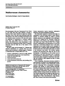
tent with AeffectsB causing the changes in the investigated system. The concept of latent Õariables ŽSection 4.1. may be seen as directly corresponding to these effects. 3.1. The data— X and Y The PLSR model is developed from a training set of N observations Žobjects, cases, compounds, process time points. with K X-variables denoted by x k Ž k s 1, . . . , K ., and M Y-variables ym Ž m s 1,2, . . . , M .. These training data form the two matrices X and Y of dimensionsŽ N ) K . and Ž N ) M ., respectively, as shown in Fig. 1. In example 1, N s 19, K s 7, and M s 1. Later, predictions for new observations are made based on their X-data. This gives predicted X-scores Ž t-values., X-residuals, their residual SD’s, and yvalues with confidence intervals. 3.2. Transformation, scaling and centering Before the analysis, the X- and Y-variables are often transformed to make their distributions be fairly symmetrical. Thus, variables with range of more than one magnitude of 10 are often logarithmically trans-
Fig. 1. Data of a PLSR can be arranged as two tables, matrices, X and Y. Note that the raw data may have been transformed Že.g., logarithmically., and usually have been centered and scaled before the analysis. In QSAR, the X-variables are descriptors of chemical structure, and the Y-variables measurements of biological activity.
113
formed. If the value zero occurs in a variable, the fourth root transformation is a good alternative to the logarithm. The response variable in example 1 is already logarithmically transformed, i.e., expressed in thermodynamic units. No further transformation was made of the example 1 data. Results of projection methods such as PLSR depend on the scaling of the data. With an appropriate scaling, one can focus the model on more important Y-variables, and use experience to increase the weights of more informative X-variables. In the absence of knowledge about the relative importance of the variables, the standard multivariate approach is to Ži. scale each variable to unit variance by dividing them by their SD’s, and Žii. center them by subtracting their averages, so-called auto-scaling. This corresponds to giving each variable Žcolumn. the same weight, the same prior importance in the analysis. In example 1, all variables were auto-scaled, except x 6 s Lam, the auto-scaling weight of which was multiplied by 1.5 to make it not be masked by the others Žso-called block-scaling.. In CoMFA and GRID-QSAR, as well as in multivariate calibration in analytical chemistry, auto-scaling is often not the best scaling of X, but non-scaled X-data or some intermediate between auto-scaled and non-scaled may be appropriate w5x. In process data, the acceptable interval of variation of each variable can form the basis for the scaling. For ease of interpretation and for numerical stability, it is recommended to center the data before the analysis. This is done—either before or after scaling —by subtracting the averages from all variables both in X and Y. In process data other reference values such as set point values may be subtracted instead of averages. Hence, the analysis concerns the deviations from the reference points and how they are related. The centering leaves the interpretation of the results unchanged. In some applications it is customary to normalize also the obserÕations Žobjects.. In chemistry, this is often done in the analysis of chromatographic or spectral profiles. The normalization is typically done by making the sum of all peaks of one profile be 100 or 1000. This removes the size of the observations Žobjects., which may be desirable if size is irrelevant. This is closely related to correspondence analysis w11x.
S. Wold et al.r Chemometrics and Intelligent Laboratory Systems 58 (2001) 109–130
114
3.3. The PLSR model
The APLS-regression coefficientsB, bm k ŽB., can be written as:
The linear PLSR model finds a few AnewB variables, which are estimates of the LV’s or their rotations. These new variables are called X-scores and denoted by t a Ž a s 1,2, . . . , A.. The X-scores are predictors of Y and also model X ŽEqs. Ž4. and Ž2. below., i.e., both Y and X are assumed to be, at least partly, modelled by the same LV’s. The X-scores are AfewB Ž A in number., and orthogonal. They are estimated as linear combinations of the original variables x k with the coefficients, AweightsB, w k)a Ž a s 1,2, . . . , A.. These weights are sometimes denoted by r k a w12,13x. Below, formulas are shown both in element and matrix form Žthe latter in parentheses.:
bm k s Ý c m a w k)a
t i a s Ý Wk)a X i k ;
Ž T s XW ) . .
Ž 1.
k
The X-scores Žt a’s. have the following properties: Ža. They are, multiplied by the loadings pa k , good AsummariesB of X, so that the X-residuals, e i k , in Eq. Ž2. are AsmallB: X i k s Ý t i a pa k q e i k ;
Ž X s TPX q E . .
Ž 2.
a
Ž 6.
a
Note that these b’s are not independent unless A Žthe number of PLSR components. equals K Žthe number of X-variables.. Hence, their confidence intervals according to the traditional statistical interpretation are infinite. An interesting special case is at hand when there is a single y-variable Ž M s 1. and XX X is diagonal, i.e., X originates from an orthogonal design Žfractional factorial, Plackett–Burman, etc... In this case there is no correlation structure in X, and PLSR arrives at the MLR solution in one component w14x, and the MLR and PLS-regression coefficients are equal to w 1 cX1. After each component, a, the X-matrix is AdeflatedB by subtracting t i)a p k a from x i k Žt a pXa from X.. This makes the PLSR model alternatively be expressed in weights wa referring to the residuals after previous dimension, E aI1 , instead of relating to the X-variables themselves. Thus, instead of Eq. Ž1., we can write: t i a s Ý wk a e i k , ay1
Ž t a s E ay1Wa .
Ž 7a .
k
With multivariate Y Žwhen M ) 1., the corresponding AY-scoresB Žu a . are, multiplied by the weights c a m , good AsummariesB of Y, so that the residuals, g i m , in Eq. Ž3. are AsmallB: yi m s Ý u i a c a m q g i m
Ž Y s UCX q G . ,
Ž 3.
a
Žb. the X-scores are good predictors of Y, i.e.: yi m s Ý c m a t i a q f i m
X
Ž Y s TC q F . .
Ž 4.
The Y-residuals, f i m express the deviations between the observed and modelled responses, and comprise the elements of the Y-residual matrix, F. Because of Eq. Ž1., Eq. Ž4. can be rewritten to look as a multiple regression model: yi m Ý c m a Ý w k)a x i k q f i m s Ý bm k x i k q f i m k
k
Ž Y s XW ) CX H F s XB H F . .
e i k , ay1 s e i k , ay2 y t i , ay1 pay1, k
Ž E ay 1 s E ay2 y t ay1 pXay1 . e i k ,0 s X i k Ž E 0 s X. .
Ž 5.
Ž 7b . Ž 7c .
However, the weights, w, can be transformed to w ) , which directly relate to X, giving Eq. Ž1. above. The relation between the two is given as w14x: W ) s W Ž PX W .
a
a
Ž B s W ) CX . .
y1
.
Ž 8.
The Y-matrix can also be AdeflatedB by subtracting t a cXa , but this is not necessary; the results are equivalent with or without Y-deflation. From the PLSR algorithm Žsee below., one can see that the first weight vector Žw 1 . is the first eigenvector of the combined variance–covariance matrix, XX YY X X, and the following weight vectors Žcomponent a. are eigenvectors to the deflated versions of the same matrix, i.e., ZXaYY X ZXa , where Z a s Z ay1 X y Tay 1 Pay1 . Similarly, the first score vector Žt 1 . is an eigenvector to XXX YY X , and later X-score vectors Žt a . are eigenvectors of Z a ZXaYY X .
S. Wold et al.r Chemometrics and Intelligent Laboratory Systems 58 (2001) 109–130
These eigenvector relationships also show that the vectors wa form an ortho-normal set, and that the vectors t a are orthogonal to each other. The loading vectors Žp a . are not orthogonal to each other, and neither are the Y-scores, u a . The u’s and the p’s are orthogonal to the t’s and the w’s, respectively, one and more components earlier, i.e., uXb t a s 0 and pXbwa s 0, if b ) a. Also, waX p a s 1.0. 3.4. Interpretation of the PLSR model One way to see PLSR is that it forms Anew xvariablesB ŽLV estimates., t a , as linear combinations of the old x’s, and thereafter uses these new t’s as predictors of Y. Hence, PLSR is based on a linear model Žsee, however, Section 4.3.. Only as many new t’s are formed as are needed, as are predictively significant ŽSection 3.8.. All parameters, t, u, w Žand w ) ., p, and c Žsee Fig. 1., are determined by a PLSR algorithm as described below. For the interpretation of the PLSR model, the scores, t and u, contain the information about the objects and their similaritiesrdissimilarities with respect to the given problem and model. The weights wa or the closely similar wa) Žsee below., and c a , give information about how the variables combine to form the quantitative relation between X and Y, thus providing an interpretation of the scores, t a and u a . Hence, these weights are essential for the understanding of which X-variables are important Žnumerically large wa-values., and which Xvariables that provide the same information Žsimilar profiles of wa-values.. The PLS weights wa express both the ApositiveB correlations between X and Y, and the Acompensation correlationsB needed to predict Y from X clear from the secondary variation in X. The latter is everything varying in X that is not primarily related to Y. This makes wa difficult to interpret directly, especially in later components Ž a ) 1.. By using an orthogonal expansion of the X-parameters in O-PLS, one can get the part of wa that primarily relates to Y, thus making the PLS interpretation more clear w15x. The part of the data that are not explained by the model, the residuals, are of diagnostic interest. Large Y-residuals indicate that the model is poor, and a normal probability plot of the residuals of a single Y-variable is useful for identifying outliers in the re-
115
lationship between T and Y, analogously to MLR. In PLSR we also have residuals for X; the part not used in the modelling of Y. These X-residuals are useful for identifying outliers in the X-space, i.e., molecules with structures that do not fit the model, and process points deviating from AnormalB process operations. This, together with control charts of the X-scores, t a , is used in multivariate SPC ŽMSPC. w16x. 3.5. Geometric interpretation PLSR is a projection method and thus has a simple geometric interpretation as a projection of the X-matrix Ža swarm of N points in a K-dimensional space. down on an A-dimensional hyper-plane in such a way that the coordinates of the projection Žt a , a s 1,2, . . . , A. are good predictors of Y. This is indicated in Fig. 2.
Fig. 2. The geometric representation of PLSR. The X-matrix can be represented as N points in the K dimensional space where each column of X Žx k . defines one coordinate axis. The PLSR model defines an A-dimensional hyper-plane, which in turn, is defined by one line, one direction, per component. The direction coefficients of these lines are pa k . The coordinates of each object, i, when its data Žrow i in X. are projected down on this plane are t i a . These positions are related to the values of Y.
116
S. Wold et al.r Chemometrics and Intelligent Laboratory Systems 58 (2001) 109–130
The direction of the plane is expressed as slopes, pa k , of each PLS direction of the plane Žeach component. with respect to each coordinate axis, x k . This slope is the cosine of the angle between the PLS direction and the coordinate axis. Thus, PLSR develops an A-dimensional hyperplane in X-space such that this plane well approximates X Žthe N points, row vectors of X., and at the same time, the positions of the projected data points on this plane, described by the scores t i a , are related to the values of the responses, activities, Yi m Žsee Fig. 2.. 3.6. Incomplete X and Y matrices (missing data) Projection methods such as PLSR tolerate moderate amounts of missing data both in X and in Y. To have missing data in Y, it must be multivariate, i.e., have at least two columns. The larger the matrices X and Y are, the higher proportion of missing data is tolerated. For small data sets with around 20 observations and 20 variables, around 10% to 20% missing data can be handled, provided that they are not missing according to some systematic pattern. The NIPALS PLSR algorithm automatically accounts for the missing values, in principle by iteratively substituting the missing values by predictions by the model. This corresponds to, for each component, giving the missing data values that have zero residuals and thus have no influence on the component parameters t a and p a . Other approaches based on the EM algorithm have been developed, and often work better than NIPALS for large percentages of missing data w17,18x. One should remember, however, that with much missing data, any resulting parameters and predictions are highly uncertain. 3.7. One Y at a time, or all in a single model? PLSR has the ability to model and analyze several Y’s together, which has the advantage to give a simpler overall picture than one separate model for each Y-variable. Hence, when the Y’s are correlated, they should be analyzed together. If the Y’s really measure different things, and thus are fairly independent, a single PLSR model tends to have many components and be difficult to interpret. Then a separate modelling of the Y’s gives a set of simpler models with fewer dimensions, which are easier to interpret.
Hence, one should start with a PCA of just the Y-matrix. This shows the practical rank of Y, i.e., the number of resulting components, A PCA . If this is small compared to the number of Y-variables Ž M ., the Y’s are correlated, and a single PLSR model of all Y’s is warranted. If, however, the Y’s cluster in strong groups, which is seen in the PCA loading plots, separate PLSR models should be developed for these groups. 3.8. The number of PLS components, A In any empirical modelling, it is essential to determine the correct complexity of the model. With numerous and correlated X-variables there is a substantial risk for Aover-fittingB, i.e., getting a well fitting model with little or no predictive power. Hence, a strict test of the predictive significance of each PLS component is necessary, and then stopping when components start to be non-significant. Cross-validation ŽCV. is a practical and reliable way to test this predictive significance w1–6x. This has become the standard in PLSR analysis, and incorporated in one form or another in all available PLSR software. Good discussions of the subject were given by Wakeling and Morris w19x and Clark and Cramer w20x. Basically, CV is performed by dividing the data in a number of groups, G, say, five to nine, and then developing a number of parallel models from reduced data with one of the groups deleted. We note that having G s N, i.e., the leave-one-out approach, is not recommendable w21x. After developing a model, differences between actual and predicted Y-values are calculated for the deleted data. The sum of squares of these differences is computed and collected from all the parallel models to form the predictive residual sum of squares ŽPRESS., which estimates the predictive ability of the model. When CV is used in the sequential mode, CV is performed on one component after the other, but the peeling off ŽEq. Ž7b., Section 3.3. is made only once on the full data matrices, where after the resulting residual matrices E and F are divided into groups for the CV of next component. The ratio PRESS arSS ay1 is calculated after each component, and a component is judged significant if this ratio is smaller than around 0.9 for at least one of the Y-variables. Slightly
S. Wold et al.r Chemometrics and Intelligent Laboratory Systems 58 (2001) 109–130
sharper bonds can be obtained from the results of Wakeling and Morris w19x. Here SS ay 1 denotes the Žfitted. residual sum of squares before the current component Žindex a.. The calculations continue until a component is non-significant. Alternatively with Atotal CVB, one first divides the data into groups, and then calculates PRESS for each component up to, say 10 or 15 with separate ApeelingB ŽEq. Ž7b., Section 3.3. of the data matrices of each CV group. The model with the number of components giving the lowest PRESSrŽ N y A y 1. is then used. This AtotalB approach is computationally more taxing, but gives similar results. Both with the AsequentialB and the AtotalB mode, a PRESS is calculated for the final model with the estimated number of significant components. This is often re-expressed as Q 2 Žthe cross-validated R 2 . which is Ž1 y PRESSrSS. where SS is the sum of squares of Y corrected for the mean. This can be compared with R 2 s Ž1 y RSSrSS., where RSS is the fitted residual sum of squares. In models with several Y’s, one obtains also R 2m and Q m2 for each Y-variable, ym . These measures can, of course, be equivalently expressed as residual SD’s ŽRSD’s. and predictive residual SD’s ŽPRESD’s.. The latter is often called standard error of prediction ŽSDEP or SEP., or standard error of cross-validation ŽSECV.. If one has some knowledge of the noise in the investigated system, for example "0.3 units for log Ž1rC . in QSAR’s, these predictive SD’s should, of course, be similar in size to the noise. 3.9. Model Õalidation Any model needs to be validated before it is used for AunderstandingB or for predicting new events such as the biological activity of new compounds or the yield and impurities at other process conditions. The best validation of a model is that it consistently precisely predicts the Y-values of observations with new X-values—a Õalidation set. But an independent and representative validation set is rare. In the absence of a real validation set, two reasonable ways of model validation are given by crossvalidation ŽCV, see Section 3.8. which simulates how well the model predicts new data, and model reestimation after data randomization which estimates
117
the chance Žprobability. to get a good fit with random response data. 3.10. PLSR algorithms The algorithms for calculating the PLSR model are mainly of technical interest, we here just point out that there are several variants developed for different shapes of the data w2,22,23x. Most of these algorithms tolerate moderate amounts of missing data. Either the algorithm, like the original NIPALS algorithm below, works with the original data matrices, X and Y Žscaled and centered.. Alternatively, so-called kernel algorithms work with the variance–covariance matrices, XX X, Y X Y, and XX Y, or association matrices, XXX and YY X , which is advantageous when the number of observations Ž N . differs much from the number of variables Ž K and M .. For extensions of PLSR, the results of Hoskulds¨ son w3x regarding the possibilities to modify the NIPALS PLSR algorithm are of great interest. Hoskuldsson shows that as long as the steps ŽC. to ŽG. below are unchanged, modifications can be made of w in step ŽB.. Central properties remain, such as orthogonality between model components, good summarizing properties of the X-scores, t a , and interpretability of the model parameters. This can be used to introduce smoothness in the PLSR solution w24x, to develop a PLSR model where a majority of the PLSR coefficients are zero w25x, align w with a` priori specified vectors Žsimilar to Atarget rotationB of Kvalheim et al. w26x., and more. The simple NIPALS algorithm of Wold et al. w2x is shown below. It starts with optionally transformed, scaled, and centered data, X and Y, and proceeds as follows Žnote that with a single y-variable, the algorithm is non-iterative.. ŽA. Get a starting vector of u, usually one of the Y columns. With a single y, u s y. ŽB. The X-weights, w: w s XX uruX u, Žhere w can now be modified. norm w to 5w 5 s 1.0 ŽC. Calculate X-scores, t: t s Xw. ŽD. The Y-weights, c: c s Y X trtX t.
S. Wold et al.r Chemometrics and Intelligent Laboratory Systems 58 (2001) 109–130
118
ŽE. Finally, an updated set of Y-scores, u: X
u s Ycrc c. ŽF. Convergence is tested on the change in t, i.e., 5t old I t new 5r5t new 5 - ´ , where ´ is AsmallB, e.g., 10y6 or 10y8 . If convergence has not been reached, return to ŽB., otherwise continue with ŽG., and then ŽA.. If there is only one y-variable, i.e., M s 1, the procedure converges in a single iteration, and one proceeds directly with ŽG.. ŽG. Remove Ždeflate, peel off. the present component from X and Y use these deflated matrices as X and Y in the next component. Here the deflation of Y is optional; the results are equivalent whether Y is deflated or not. p s XX tr Ž tX t . X s X y tpX Y s Y y tcX . ŽH. Continue with next component Žback to step . A until cross-validation Žsee above. indicates that there is no more significant information in X about Y. Chu et al. w27x recently has reviewed the attractive properties of matrix decompositions of the Wedderburn type. The PLSR NIPALS algorithm is such a Wedderburn decomposition, and hence is numerically and statistically stable. 3.11. Standard errors and confidence interÕals Numerous efforts have been made to theoretically derive confidence intervals of the PLSR parameters, see, e.g., Ref. w28x. Most of these are, however, based on regression assumptions, seeing PLSR as a biased regression model. Only recently, in the work of Burnham et al. w12x, have these matters been investigated with PLSR as a latent Õariable regression model. A way to estimate standard errors and confidence intervals directly from the data is to use jack-knifing w29x. This was recommended by Wold w1x in his original PLS work, and has recently been revived by Martens and Martens w30x and others. The idea is simple; the variation in the parameters of the various sub-models obtained during cross-validation is used to derive their standard deviations Žcalled standard
errors., followed by using the t-distribution to give confidence intervals. Since all PLSR parameters Žscores, loadings, etc.. are linear combinations of the original data Žpossibly deflated., these parameters are close to normally distributed, and hence jack-knifing works well.
4. Assumptions underlying PLSR 4.1. Latent Variables In PLS modelling, we assume that the investigated system or process actually is influenced by just a few underlying variables, latent Õariables (LV’s). The number of these LV’s is usually not known, and one aim with the PLSR analysis is to estimate this number. Also, the PLS X-scores, t a , are usually not direct estimates of the LV’s, but rather they span the same space as the LV’s. Thus, the latter Ždenoted by V. are related to the former ŽT. by a, usually unknown, rotation matrix, R, with the property RX R s 1: V s TRX or T s RV. Both the X- and the Y-variables are assumed to be realizations of these underlying LV’s, and are hence not assumed to be independent. Interestingly, the LV assumptions closely correspond to the use of microscopic concepts such as molecules and reactions in chemistry and molecular biology, thus making PLSR philosophically suitable for the modelling of chemical and biological data. This has been discussed by, among others, Wold et al. w31,32x, Kvalheim w33x, and recently from a more fundamental perspective, by Burnham et al. w12,13x. In spectroscopy, it is clear that the spectrum of a sample is the sum of the spectra of the constituents multiplied by their concentrations in the sample. Identifying the latter with t ŽLambert– Beers AlawB ., and the spectra with p, we get the latent variable model X s t1p1X q t2p2X q . . . s TPX q noise. In many applications this interpretation with the data explained by a number of AfactorsB Žcomponents. makes sense. As discussed below, we can also see the scores, T, as comprised of derivatives of an unknown function underlying the investigated system. The choice of the interpretation depends on the amount of knowledge
S. Wold et al.r Chemometrics and Intelligent Laboratory Systems 58 (2001) 109–130
about the system. The more knowledge we have, the more likely it is that we can assign a latent variable interpretation of the X-scores or their rotation. If the number of LV’s actually equals the number of X-variables, K, then the X-variables are independent, and PLSR and MLR give identical results. Hence, we can see PLSR as a generalization of MLR, containing the latter as a special case in situations when the MLR solution exists, i.e., when the number of X- and Y-variables is fairly small in comparison to the number of observations, N. In most practical cases, except when X is generated according to an experimental design, however, the X-variables are not independent. We then call X rank deficient. Then PLSR gives a AshrunkB solution which is statistically more robust than the MLR solution, and hence gives better predictions than MLR w34x. PLSR gives a model of X in terms of a bilinear projection, plus residuals. Hence, PLSR assumes that there may be parts of X that are unrelated to Y. These parts can include noise andror regularities non-related to Y. Hence, unlike MLR, PLSR tolerates noise in X. 4.2. AlternatiÕe deriÕation The second theoretical foundation of LV-models is one of Taylor expansions w35x. We assume the data X and Y to be generated by a multi-dimensional function F Žu,v., where the vector variable u describes the change between observations Žrows in X. and the vector variable v describes the change between variables Žcolumns in X.. Making a Taylor expansion of the function F in the u-direction, and discretizing for i s observation and k s variable, gives the LV-model. Again, the smaller the interval of u that is modelled, the fewer terms we need in the Taylor expansion, and the fewer components we need in the LV-model. Hence, we can interpret PCA and PLS as models of similarity. Data Žvariables. measured on a set of similar observations Ž samples, items, cases, . . . . can always be modelled Žapproximated. by a PC- or PLS model. And the more similar are the observations, the fewer components we need in the model. We hence have two different interpretations of the LV-model. Thus, real data well explained by these models can be interpreted as either being a linear combination of AfactorsB or according to the latter
119
interpretation as being measurements made on a set of similar observations. Any mixture of these two interpretations is, of course, often applicable. 4.3. Homogeneity Any data analysis is based on an assumption of homogeneity. This means that the investigated system or process must be in a similar state throughout all the investigation, and the mechanism of influence of X on Y must be the same. This, in turn, corresponds to having some limits on the variability and diversity of X and Y. Hence, it is essential that the analysis provides diagnostics about how well these assumptions indeed are fulfilled. Much of the recent progress in applied statistics has concerned diagnostics w36x, and many of these diagnostics can be used also in PLSR modelling as discussed below. PLSR also provides additional diagnostics beyond those of regression-like methods, particularly those based on the modelling of X Žscore and loading plots and X-residuals.. In the first example, the first PLSR analysis indicated that the data set was inhomogeneous—three aromatic amino acids ŽAA’s. are indicated to have a different type of effect than the others on the modelled property. This type of information is difficult to obtain in ordinary regression modelling, where only large residuals in Y provide diagnostics about inhomogeneities. 4.4. Non-linear PLSR For non-linear situations, simple solutions have w4x, and Berglund and been published by Hoskuldsson ¨ Wold w37x. Another approach based on transforming selected X-variables or X-scores to qualitative variables coded as sets of dummy variables, the so-called GIFI approach w38,39x, is described elsewhere in this volume w15x. 5. Results of example 1 5.1. The initial PLSR analysis of the AA data The first PLSR analysis Žlinear model. of the AA data gives one significant component explaining 43% of the Y-variance Ž R 2 s 0.435, Q 2 s 0.299.. In contrast, the MLR gives an R 2 of 0.788, which is equiv-
120
S. Wold et al.r Chemometrics and Intelligent Laboratory Systems 58 (2001) 109–130
Fig. 3. The PLS scores u 1 and t 1 of the AA example, 1st analysis.
alent to PLSR with A s 7 components. The full MLR solution, however, has a Q 2 of y0.215, indicating that the model is poor, and does not predict better than chance. With just one significant PLS component, the only meaningful score plot is that of y against t ŽFig. 3.. The aromatic AA’s, Trp, Phe, and, may be, Tyr, show a much worse fit than the others, indicating an inhomogeneity in the data. To investigate this, a second round of analysis is made with a reduced data set, N s 16, without the aromatic AA’s. 5.2. Second analysis The modelling of N s 16 AA’s with the same linear model as before gives a substantially better result
with A s 2 significant components and R 2 s 0.783, Q 2 s 0.706. The MLR model for these 16 objects gives a R 2 of 0.872, and a Q 2 of 0.608. This strong improvement indicates that indeed the data set now is more homogeneous and can be properly modelled. The plot in Fig. 4 of u 1 Žy. vs. t 1 shows, however, a fairly strong curvature, indicating that squared terms in lipophilicity and, may be, polarity are warranted. In the final analysis, the squares of these four variables were included in the model, which indeed gave better results. Two significant PLS components and one additional with border-line significance were obtained. The resulting R 2 and Q 2 values are for A s 2: 0.90 and 0.80, and for A s 3: 0.925 and 0.82, respectively. The A s 3 values correspond to RSD s 0.92, and PRESD ŽSDEP. s 1.23, since the SD of Y
Fig. 4. The PLS scores, u 1 and t 1 of the AA example, 2nd analysis.
S. Wold et al.r Chemometrics and Intelligent Laboratory Systems 58 (2001) 109–130
121
Fig. 5. The PLS scores t 1 and t 2 of the AA example, 2nd analysis. The overlapping points up to the right are Ile and Leu.
is 2.989. The full MLR model gives R 2 s 0.967, but with much worse Q 2 s 0.09. 5.2.1. X-scores (t a ) show object similarities and dissimilarities The plot of the X-scores Žt 1 vs. t 2 , Fig. 5. shows the 16 amino acids grouped according to polarity from upper left to lower right, and inside each group, according to size and lipophilicity. 5.2.2. PLSR weights w and c For the interpretation of PLSR models, the standard is to plot the w ) ’s and c’s of one model dimension against another. Alternatively, one can plot the
w’s and c’s; the results and interpretation is similar. This plot shows how the X-variables combine to form the scores t a ; X-variables important for the ath component fall far from the origin along the ath axis in the wc-plot. Analogously, Y-variables well modelled by the ath component have large coefficients, c a m , and hence fall far from the origin along the ath axis in the same plot. The example 1 weight plot ŽFig. 6, often also called loading plot. shows the first PLS component dominated by lipophilicity and polarity ŽPIF, PIE, and Lam on the positive side, and DGR on the negative., and the second component being a mixture of size and polarity with MR, Vol, and SAC on the positive Žhigh. side, and Lam on the negative Žlow. side.
Fig. 6. The PLS weights, w ) and c for the first two dimensions of the 2nd AA model.
122
S. Wold et al.r Chemometrics and Intelligent Laboratory Systems 58 (2001) 109–130
Fig. 7. PLS regression coefficients after A s 2 components Žsecond analysis.. The bars indicate 95% confidence intervals based on jackknifing.
The c-values of the response, y, are proportional to the linear variation of Y explained by the corresponding dimension, i.e., R 2 . They define one point per response; in the example with a single response, this point ŽDDGTS. sits far to the right in the first quadrant of the plot. The importance of a given X-variable for Y is proportional to its distance from the origin in the loading space. These lengths correspond to the PLSregression coefficients after A s 2 dimensions ŽFig. 7.. 5.3. Comparison with multiple linear regression (MLR) Comparing the PLS model Ž A s 2. and the MLR model Žequivalent to the PLS model with A s 7.
shows that the coefficients of x 3 ŽDGR. and x 4 ŽSAC. change sign between the PLSR model ŽFig. 7. and the MLR model ŽFig. 8.. Moreover, the coefficients of x 4 , x 5 , and x 7 which are moderate in the PLSR Ž A s 2. model become large and with opposite signs in the MLR model Ž A s 7., although they are strongly positively correlated to each other in the raw data. The MLR coefficients clearly are misleading and un-interpretable, due to the strong correlations between the X-variables. PLSR, however, stops at A s 2, and gives reasonable coefficient values both for A s 2 and A s 3. With correlated variables one cannot assign AcorrectB values to the individual coefficients, the only thing we can estimate is their joint contribution to y.
Fig. 8. The MLR coefficients corresponding to analysis 2. The bars indicate 95% confidence intervals based on jack-knifing. Note the differences in the vertical scale to Fig. 7.
S. Wold et al.r Chemometrics and Intelligent Laboratory Systems 58 (2001) 109–130
123
Fig. 9. VIP of the X-variables of the three-component PLSR model, 3rd analysis. The squares of x 1 s PIE, x 2 s PIF, x 3 s DGR, and x 6 s Lam, are denoted by S1)1, S2)2, S3)3, and S6)6, respectively.
5.4. Measures of Õariable importance
5.5. Residuals
In PLSR modelling, a variable Žx k . may be important for the modelling of Y. Such variables are identified by large PLS-regression coefficients, bm k . However, a variable may also be important for the modelling of X, which is identified by large loadings, pa k . A summary of the importance of an Xvariable for both Y and X is given by VIPk Žvariable importance for the projection, Fig. 9.. This is a weighted sum of squares of the PLS-weights, wa)k , with the weights calculated from the amount of Yvariance of each PLS component, a.
The residuals of Y and X ŽE and F in Eqs. Ž2. and Ž4. above. are of diagnostic value for the quality of the model. A normal probability plot of the Y-residuals ŽFig. 10. of the final AA model shows a fairly straight line with all values within "3 SD’s. To be a serious outlier, a point should clearly deviate from the line, and be outside "4 SD’s. Since the X-residuals are many Ž N ) K ., one needs a summary for each observation Žcompound. not to drown in details. This is provided by the residual SD of the X-residuals of the corresponding row
Fig. 10. Y-residuals of the three-component PLSR model, 3rd analysis, normal probability plot.
124
S. Wold et al.r Chemometrics and Intelligent Laboratory Systems 58 (2001) 109–130
of the residual matrix E. Because this SD is proportional to the distance between the data point and the model plane in X-space, it is also often called DModX Ždistance to the model in X-space.. A DModX larger than around 2.5 times the overall SD of the X-residuals Žcorresponding to an F-value of 6.25. indicates that the observation is an outlier. Fig. 11 shows that none of the 16 compounds in example 1 has a large DModX. Here the overall SD s 0.34. 5.6. Conclusions of example 1 The initial PLSR analysis gave diagnostics Žscore plots. that indicated in-homogeneities in the data. A much better model was obtained for the N s 16 non-aromatic AA’s. A remaining curvature in the score plot of u 1 vs. t 1 lead to the inclusion of squared terms, which gave a good final model. Only the squares in the lipophilicity variables are significant in the final model. If additional aromatic AA’s had been present, a second separate model could have been developed for this type of AA’s. This would provide insight in how this aromatic group differs from the non-aromatic AA’s. This is, in a way, a non-linear model of the changes in the relationship between structure and activity when going from non-aromatic to aromatic AA’s. These changes are too large and non-linear to be modelled by a linear or low degree polynomial model. The use of two separate models, which do not
directly model the change from one group to another, provides a simple approach to deal with these nonlinearities.
6. Example 2 (SIMCODM) High and consistent product quality combined with AgreenB plant operation is important in today’s competitive industrial climate. The goal of process data modelling is often to reduce the amount of down time and eliminate sources of undesired and deleterious process variability. The second example shows the investigation of possibilities to operate a process industry in an environment-friendly manner w40x. At the Aylesford Newsprint paper-mill in Kent, UK, premium quality newsprint is produced from 100% recycled fiber, i.e., reclaimed newspapers and magazines. The first step of the process is one of deinking. This has stages of cleaning, screening, and flotation. First the wastepaper is fed into rotating drum pulpers, where it is mixed with warm water and chemicals to initiate the fiber separation and ink removal. In the next stage, the pulp undergoes prescreening and cleaning to remove light and heavy contaminants Žstaples, paper clips, sand, plastics, etc... Thereafter the pulp goes to a pre-flotation stage. After the pre-flotation the pulp is thickened and dispersed and the brightness is adjusted. After post-flotation and washing the de-inked pulp ŽDIP. is sent via
Fig. 11. RSD’s of each compound’s X-residuals ŽDModX., 3rd analysis.
S. Wold et al.r Chemometrics and Intelligent Laboratory Systems 58 (2001) 109–130
storage towers to the paper machines for production of premium quality newsprint. The wastewater discharged from the de-inking process is the main source of chemical oxygen demand ŽCOD. of the mill effluent. COD estimates the oxygen requirements of organic matter present in the effluent. The COD in the effluent is reduced by 85% prior to discharge to the river Medway. Stricter environmental regulations and costs of COD reduction made the investigation of the COD sources and possible control strategies one of the company’s environmental objectives for 1999. A multivariate approach was adopted. Thus, data from more than a year were used in the multivariate study. The example data set contains 384 daily observations, with one response variable ŽCOD load, y 1 . and 54 process variables Ž x 2 y x 55 .. Half of the observations Žprocess time points. are used for model training and half for model validation.
125
Fig. 13. Example 2. PCA loading plot Žp1rp2. corresponding to Fig. 12. The position of the COD load, variable number 1, is highlighted by an increased font size.
6.1. OÕerÕiew by PCA PCA applied to the entire data set ŽX and Y. gave an eight-component model explaining R 2 s 79% and predicting Q 2 s 68% of the data variation. Scores and loadings of the first two components accounting for 54% of the sum of squares are plotted in Figs. 12 and 13.
Fig. 12 reveals a main cluster in the right-hand part of the score plot, where the process has spent most of its time. Occasionally, the process has drifted away towards the left-hand area of the score plot, corresponding to a lower production rate, including planned shut downs in one of the process lines. The loading plot shows most of the variables having low numerical values Ži.e., low material flow, low addition of process chemicals, etc.. for the low production rates. This analysis shows that the data are not strongly clustered. The low production process time points deviate from the main cluster, but not seriously. Rather, the inclusion of the low production time points in the subsequent PLSR modelling give a good spanning of key features such as brightness, residual ink, and addition of external chemicals. 6.2. Selection of training set for PLSR and lagging of data
Fig. 12. Example 2. PCA score plot Žt1rt2. of overview model. Each point represents one process time point.
The parent data set, with preserved time order, was split into two halves, one training set and one prediction set. Only forward prediction was applied. Process insight, initial PLSR modelling, and inspection of cross-correlations, indicated that lagging 10 of the variables was warranted to catch process dynamics.
126
S. Wold et al.r Chemometrics and Intelligent Laboratory Systems 58 (2001) 109–130
6.3. PLSR modelling PLSR was utilized to relate the 54 q 10 process variables to the COD load. A two-component PLSR model was obtained, with R 2X s 0.49, R 2Y s 0.60, Q Y2 ŽCV. s 0.57, and Q Y2 Žext. s 0.59 Žexternal validation set.. Fig. 14 shows relationships between observed and predicted levels of COD for the validation set. The picture for the training set is very similar. 6.4. Results
Fig. 14. Example 2. Observed verses predicted COD for the prediction set.
These were: lags 1–4 of COD, and lags 1 and 2 of variables x 23 , x 24 Žaddition of two chemicals., and x 35 Ža flow., totally 10 lagged X’s. Lagging a variable L steps means that the same variable shifted L steps in time is included as an additional variable in the data set.
The collected process variables together with their lags predict COD load with Q 2 ) 0.6. This is a satisfying result considering the complexity of the process and the great variations that occur in the starting material Žrecycled paper.. The PLS-regression coefficients ŽFig. 15., show the process variables with the strongest correlation to the COD load to be x 23 , x 24 Žaddition of chemicals., x 34 , x 35 Žflows., and x 49 and x 50 Žtemperatures., with coefficients exceeding 0.04. Only some of these can be controlled, namely x 23 , x 24 , and x 49 . More-
Fig. 15. Example 2. Plot of regression coefficients of scaled and centered variables of PLS model. Coefficients with numbers 2 to 55 represent the 54 original process variables. Coefficients 57–60 depict lags 1–4 of COD, and coefficients 61–66 the two first lags of variables x 23 , x 24 , and x 35 .
S. Wold et al.r Chemometrics and Intelligent Laboratory Systems 58 (2001) 109–130
over, the lagged variables are important. Variables 57–60 are the four first lags of the COD variable. Obviously, past measurements of COD are useful for modelling and predicting future levels of COD—the change in this variable is slow. The variables 61–66 are lags 1 and 2 of x 23 , x 24 , and x 35 . The dynamics of these process variables are thus related to COD. Unfortunately, none of the three controlled variables Ž x 23 , x 24 , and x 49 . offer a means to decrease COD. The former two variables describe the addition of caustic and peroxide to the dispergers, and cannot be significantly reduced without endangering pulp quality. The last variable is the raw effluent temperature which cannot be lowered without negative effects on pulp quality. This result is typical for the analysis of historical process data. The value of the analysis is mainly to detect deviations from normal operation, not as a means to process optimization. The latter demands data from a statistically designed set of experiments with the purpose of optimizing the process.
7. Summary; how to develop and interpret a PLSR model Ž1. Have a good understanding of the stated problem, particularly which responses Žproperties., Y, that are of interest to measure and model, and which predictors, X, that should be measured and varied. If possible, i.e., if the X-variables are subject to experimental control, use statistical experimental design w41x for the construction of X. Ž2. Get good data, both Y Žresponses. and X Žpredictors.. Multivariate Y’s provide much more information because they can first be separately analyzed by a PCA. This gives a good idea about the amount of systematic variation in Y, which Y-variables that should be analyzed together, etc. Ž3. The first piece of information about the model is the number of significant components, A—the complexity of the model and hence of the system. This number of components gives a lower bound of the number of effects we need to postulate in the system. Ž4. The goodness of fit of the model is given by 2 R and Q 2 Žcross-validated R 2 .. With several Y’s,
127
one obtains also R 2m and Q m2 for each ym . The R 2 ’s give an upper bound of how well the model explains the data and predicts new observations, and the Q 2 ’s give lower bounds for the same things. Ž5. The Žu,t. score plots for the first two or three model dimensions will show the presence of outliers, curvature, or groups in the data. The Žt,t. score plots—windows in X-space—show in-homogeneities, groups, or other patterns. Together with this, the Žw ) c. weight plots gives an interpretation of these patterns. Ž6a. If problems are seen, i.e., small R 2 and Q 2 values, or outliers, groups, or curvature in the score plots, one should try to remedy the problem. Plots of residuals Žnormal probability and DModX and DModY. may give additional hints for the sources of the problems. Single outliers should be inspected for correctness of data, and if this does not help, be excluded from the analysis only if they are non-interesting Ži.e., low activity.. Curvature in Žu,t. plots may be improved by transforming parts of the data Že.g., log., or by including squared andror cubic terms in the model. After possibly having transformed the data, modified the model, divided the data into groups, deleted outliers, or whatever warranted, one returns to step 1. Ž6b. If no problems are seen, i.e., R 2 and Q 2 are OK, and the model is interpretable, one may try to mildly prune the model by deleting unimportant terms, i.e., with small regression coefficients and low VIP values. Thereafter a final model is developed, interpreted, and validated, predictions are made, etc. For the interpretation the Žw ) c. weight plots, coefficient plots, and contour or 3D plots with dominating X’s as plot coordinates, are invaluable.
8. Regression-like data-analytical problems A number of seemingly different data-analytical problems can be expressed as regression problems with a special coding of Y or X. These include linear discriminant analysis ŽLDA., analysis of variance ŽANOVA., and time series analysis ŽARMA and similar models.. With many and collinear variables Žrank-deficient X., a PLSR solution can therefore be formulated for each of these.
128
S. Wold et al.r Chemometrics and Intelligent Laboratory Systems 58 (2001) 109–130
In linear discriminant analysis ŽLDA., and the closely related canonical variates analysis ŽCVA., one has the X-matrix divided in a number of classes, with index 1,2, . . . , g, . . . ,G. The objective of the analysis is to find linear combinations of the X-variables Ždiscriminant functions. that discriminate between the classes, i.e., have very different values for the classes w11x. Provided that each class is AtightB and occupies a small and separate volume in X-space, one can find a plane—a discriminant plane—in which the projected observations are well separated according to class. With many and collinear X-variables, a PLS version of LDA ŽPLS-DA. is useful w42,43x. However, when some of the classes are not tight, often due to a lack of homogeneity and similarity in these non-tight classes, the discriminant analysis does not work. Then other approaches, such as, SIMCA have to be used, where a PC or PLSR model is developed for each tight class, and new observations are classified according to their nearness in X-space to these class models. Analogously, when X contains qualitative variables Žthe ANOVA situation., these can be coded using dummy variables, and the data then analyzed using MLR or PLSR. The latter is advantageous if the coded X is unbalanced andror rank deficient Žor close to.. With several Y-variables, this provides a simple approach to MANOVA Žmultiple responses ANOVA. w11x. Auto-regressive and transfer function models in time-series analysis are easily analyzed by first constructing an expanded X-matrix that contains the appropriate lags of Y- and X-variables, and then calculating a PLSR solution. If the disturbances a t are included in the models ŽARMA, etc.., a two-step analysis is needed, first calculating estimates of a t , and then using these in lagged forms in the final PLSR model. In the modelling of mixtures, for instance of chemical ingredients in paints, pharmaceutical, cosmetic, and polymer formulations, beverages, etc., the sum of the X-variables is 1.0, since ingredients sum to 100%. This makes X rank deficient, and a number of special regression approaches have been developed for the analysis of mixture data. With PLSR, however, the rank deficiency presents no difficulties, and the data analysis becomes straight forward, as shown by Kettaneh-Wold w44x.
The iterative calculations in non-linear regression often involve a regression-like updating step Že.g., the Gauss–Newton approach.. The X-matrix of this step is often highly rank-deficient, and ridge-regression is used to remedy the situation ŽMarquardt–Lefwenberg algorithms.. PLSR provides a simple and interesting alternative, which also is computationally very fast.
9. Conclusions and discussion PLSR provides an approach to the quantitative modelling of the often complicated relationships between predictors, X, and responses, Y, that with complex problems often is more realistic than MLR including stepwise selection variants. This because the assumptions underlying PLS — correlations among the X’s, noise in X, model errors—are more realistic than the MLR assumptions of independent and error free X’s. The diagnostics of PLSR, notably cross-validation and score plots Žu, t and t, t. with corresponding loading plots, provide information about the correlation structure of X that is not obtained in ordinary MLR. In particular, PLSR results showing that the data are inhomogeneous Žlike the AA example looked at here., are hard to obtain by MLR. In complicated systems, non-linearities so strong that a single polynomial model cannot be constructed, seem to be rather common. Hence, a flexible approach to modelling is often warranted with separate models for different mechanistic classes. And there is no loss of information with this approach in comparison with the single model approach. A new observation Žobject. is first classified with respect to its X-values, and predicted response values are then obtained by the appropriate class model. The ability of PLSR to analyze profiles of responses, makes it easier to device response measurements that are relevant to the stated objective of the investigation; it is easier to capture the behavior of a complicated system by a battery of measurements than by a single variable. PLSR can be extended in various directions, to non-linear modelling, hierarchical modelling when the variables are very numerous, multi-way data, PLS time series, PLS-DA, etc. Many recently developed
S. Wold et al.r Chemometrics and Intelligent Laboratory Systems 58 (2001) 109–130
PLS based approaches are discussed in other articles in this volume. The statistical understanding of PLSR has recently improved substantially w12,13,34x. We feel that the flexibility of the PLS-approach, its graphical orientation, and its inherent ability to handle incomplete and noisy data with many variables Žand observations. makes PLS a simple but powerful approach for the analysis of data of complicated problems.
Acknowledgements Support from the Swedish Natural Science Research Council ŽNFR., and from the Center for Environmental Research in Umea˚ ŽCMF. is gratefully acknowledged. Dr. Erik Johansson is thanked for helping with the examples.
References w1x H. Wold, Soft modelling, The basic design and some extensions, in: K.-G. Joreskog, H. Wold ŽEds.., Systems Under In¨ direct Observation, vols. I and II, North-Holland, Amsterdam, 1982. w2x S. Wold, A. Ruhe, H. Wold, W.J. Dunn III, The collinearity problem in linear regression, The partial least squares approach to generalized inverses, SIAM J. Sci. Stat. Comput. 5 Ž1984. 735–743. w3x A. Hoskuldsson, PLS regression methods, J. Chemom. 2 ¨ Ž1988. 211–228. w4x A. Hoskuldsson, Prediction Methods in Science and Technol¨ ogy, vol. 1, Thor Publishing, Copenhagen, 1996, ISBN 87985941-0-9. w5x S. Wold, E. Johansson, M. Cocchi, PLS—partial least squares projections to latent structures, in: H. Kubinyi ŽEd.., 3D QSAR in Drug Design, Theory, Methods, and Applications, ESCOM Science Publishers, Leiden, 1993, pp. 523–550. w6x M. Tenenhaus, La Regression PLS: Theorie et Pratique, Technip, Paris, 1998. w7x R.W. Gerlach, B.R. Kowalski, H. Wold, Partial least squares modelling with latent variables, Anal. Chim. Acta 112 Ž1979. 417–421. w8x N.E. El Tayar, R.-S. Tsai, P.-A. Carrupt, B. Testa, Octan-1ol-water partition coefficients of zwitterionic a-amino acids, Determination by centrifugal partition chromatography and factorization into stericrhydrophobic and polar components, J. Chem. Soc., Perkin Trans. 2 Ž1992. 79–84. w9x S. Hellberg, M. Sjostrom, ¨ ¨ S. Wold, The prediction of bradykinin potentiating potency of pentapeptides, An example of a peptide quantitative structure–activity relationship, Acta Chem. Scand., Ser. B 40 Ž1986. 135–140.
129
w10x M. Sandberg, L. Eriksson, J. Jonsson, M. Sjostrom, ¨ ¨ S. Wold, New chemical dimensions relevant for the design of biologically active peptides, A multivariate characterization of 87 amino acids, J. Med. Chem. 41 Ž1998. 2481–2491. w11x J.E. Jackson, A User’s Guide to Principal Components, Wiley, New York, 1991. w12x A.J. Burnham, J.F. MacGregor, R. Viveris, Latent variable regression tools, Chemom. Intell. Lab. Syst. 48 Ž1999. 167– 180. w13x A. Burnham, R. Viveros, J. MacGregor, Frameworks for latent variable multivariate regression, J. Chemom. 10 Ž1996. 31–45. w14x R. Manne, Analysis of two partial least squares algorithms for multivariate calibration, Chemom. Intell. Lab. Syst. 1 Ž1987. 187–197. w15x J. Trygg et al., This issue. w16x P. Nomikos, J.F. MacGregor, Multivariate SPC charts for monitoring batch processes, Technometrics 37 Ž1995. 41–59. w17x P.R.C. Nelson, P.A. Taylor, J.F. MacGregor, Missing data methods in PCA and PLS: score calculations with incomplete observation, Chemom. Intell. Lab. Syst. 35 Ž1996. 45–65. w18x B. Grung, R. Manne, Missing values in principal component analysis, Chemom. Intell. Lab. Syst. 42 Ž1998. 125–139. w19x I.N. Wakeling, J.J. Morris, A test of significance for partial least squares regression, J. Chemom. 7 Ž1993. 291–304. w20x M. Clark, R.D. Cramer III, The probability of chance correlation using partial least squares ŽPLS., Quant. Struct.-Act. Relat. 12 Ž1993. 137–145. w21x J. Shao, Linear model selection by cross-validation, J. Am. Stat. Assoc. 88 Ž1993. 486–494. w22x F. Lindgren, P. Geladi, S. Wold, The kernel algorithm for PLS I, Many observations and few variables, J. Chemom. 7 Ž1993. 45–59. w23x S. Rannar, P. Geladi, F. Lindgren, S. Wold, The kernel algo¨ rithm for PLS II, Few observations and many variables, J. Chemom. 8 Ž1994. 111–125. w24 x K.H. Esbensen, S. Wold, SIMCA, MACUP, SELPLS, GDAM, SPACE and UNFOLD: the ways towards regionalized principal components analysis and subconstrained N-way decomposition—with geological illustrations, in: O.J. Christie ŽEd.., Proc. Nord. Symp. Appl. Statist. Stavanger, 1983, pp. 11–36, ISBN 82-90496-02-8. w25x N. Kettaneh-Wold, J.F. MacGregor, B. Dayal, S. Wold, Multivariate design of process experiments ŽM-DOPE., Chemom. Intell. Lab. Syst. 23 Ž1994. 39–50. w26x O.M. Kvalheim, A.A. Christy, N. Telnaes, A. Bjoerseth, Maturity determination of organic matter in coals using the methylphenantrene distribution, Geochim. Cosmochim. Acta 51 Ž1987. 1883–1888. w27x M.T. Chu, R.E. Funderlic, G.H. Golub, A rank-one reduction formula and its applications to matrix factorizations, SIAM Rev. 37 Ž1995. 512–530. w28x M.C. Denham, Prediction intervals in partial least squares, J. Chemom. 11 Ž1997. 39–52. w29x B. Efron, G. Gong, A leisurely look at the bootstrap, the jackknife, and cross-validation, Am. Stat. 37 Ž1983. 36–48. w30x H. Martens, M. Martens, Modified jack-knife estimation of
130
w31x
w32x
w33x w34x
w35x
w36x
S. Wold et al.r Chemometrics and Intelligent Laboratory Systems 58 (2001) 109–130 parameter uncertainty in bilinear modeling ŽPLSR., Food Qual. Preference 11 Ž2000. 5–16. S. Wold, C. Albano, W.J. Dunn III, U. Edlund, B. Eliasson, E. Johansson, B. Norden, M. Sjostrom, ¨ ¨ The indirect observation of molecular chemical systems, in: K.-G. Joreskog, H. ¨ Wold ŽEds.., Systems Under Indirect Observation, vols. I and II, North-Holland, Amsterdam, 1982, pp. 177–207, Chapter 8. S. Wold, M. Sjostrom, ¨ ¨ L. Eriksson, PLS in chemistry, in: P.v.R. Schleyer, N.L. Allinger, T. Clark, J. Gasteiger, P.A. Kollman, H.F. Schaefer III, P.R. Schreiner ŽEds.., The Encyclopedia of Computational Chemistry, Wiley, Chichester, 1999, pp. 2006–2020. O. Kvalheim, The latent variable, an editorial, Chemom. Intell. Lab. Syst. 14 Ž1992. 1–3. I.E. Frank, J.H. Friedman, A statistical view of some chemometrics regression tools, With discussion, Technometrics 35 Ž1993. 109–148. S. Wold, A theoretical foundation of extrathermodynamic relationships Žlinear free energy relationships., Chem. Scr. 5 Ž1974. 97–106. D.A. Belsley, E. Kuh, R.E. Welsch, Regression Diagnostics: Identifying Influential Data and Sources of Collinearity, Wiley, New York, 1980.
w37x A. Berglund, S. Wold, INLR, implicit non-linear latent variable regression, J. Chemom. 11 Ž1997. 141–156. w38x S. Wold, A. Berglund, N. Kettaneh, N. Bendwell, D.R. Cameron, The GIFI approach to non-linear PLS modelling, J. Chemom. 15 Ž2001. 321–336. w39x L. Eriksson, E. Johansson, F. Lindgren, S. Wold, GIFI-PLS: modeling of non-linearities and discontinuities in QSAR, QSAR 19 Ž2000. 345–355. w40x L. Eriksson, P. Hagberg, E. Johansson, S. Rannar, D. Sarney, ¨ ˚ ¨ T. Lindgren, Multivariate process O. Whelehan, A. Astrom, monitoring of a newsprint mill, Application to modelling and predicting COD load resulting from de-inking of modeling, J. Chemom. 15 Ž2001. 337–352. w41x G.E.P. Box, W.G. Hunter, J.S. Hunter, Statistics for Experimenters, Wiley, New York, 1978. w42x M. Sjostrom, ¨ ¨ S. Wold, B. Soderstrom, ¨ ¨ PLS discriminant plots, Proceedings of PARC in Practice, Amsterdam, June 19–21, 1985, Elsevier, North-Holland, 1986, pp. 461–470. w43x L. Stahle, S. Wold, Partial least squares analysis with cross˚ validation for the two-class problem: a Monte Carlo study, J. Chemom. 1 Ž1987. 185–196. w44x N. Kettaneh-Wold, Analysis of mixture data with partial least squares, Chemom. Intell. Lab. Syst. 14 Ž1992. 57–69.