the boundary point interpolation method (BPIM) (Gu and Liu 2002). Detailed discussion of meshless methods can be found in the book of Liu (2002b).GAmong ...
Structural Engineering and Mechanics, Vol. 14, No. 6 (2002) 713-732
713
Point interpolation method based on local residual formulation using radial basis functions G.R. Liu†, L. Yan‡, J.G. Wang†‡ and Y.T. Gu‡‡ Center for Advanced Computation in Engineering Science, Department of Mechanical and Production Engineering, National University of Singapore, 10 Kent Ridge Crescent, Singapore 119260
(Received December 28, 2001, Revised October 8, 2002, Accepted November 13, 2002) Abstract. A local radial point interpolation method (LRPIM) based on local residual formulation is presented and applied to solid mechanics in this paper. In LRPIM, the trial function is constructed by the radial point interpolation method (PIM) and establishes discrete equations through a local residual formulation, which can be carried out nodes by nodes. Therefore, element connectivity for trial function and background mesh for integration is not necessary. Radial PIM is used for interpolation so that singularity in polynomial PIM may be avoided. Essential boundary conditions can be imposed by a straightforward and effective manner due to its Delta properties. Moreover, the approximation quality of the radial PIM is evaluated by the surface fitting of given functions. Numerical performance for this LRPIM method is further studied through several numerical examples of solid mechanics. Key words: meshless method; radial basis function; point interpolation; background integration.
1. Introduction Meshless method has attracted more and more attention from researchers in recent years, and it is regarded as a potential numerical method in computational mechanics. As it abandons the concept of element, it alleviates some problems associated with the finite element method, such as mesh locking, element distortion, re-meshing procedure during large deformations, and so on. Several meshless methods have been developed, such as the smooth particle hydrodynamics (SPH) (Gingold and Monaghan 1977); the element free Galerkin method (EFG) (Belytschko et al. 1994, 1996); the meshless local Petrov-Galerkin method (MLPG) (Atluri and Zhu 1998, Atluri et al. 1999); the point assemble method (PAM) (Liu 2002a); the point interpolation method (PIM) (Liu and Gu 2001) and the boundary point interpolation method (BPIM) (Gu and Liu 2002). Detailed discussion of meshless methods can be found in the book of Liu (2002b).GAmong all these meshless methods, the MLPG does not require any mesh not only for the purpose of interpolation of field variables, but also for the integration of the weak form of equilibrium equations. The MLPG method is a newly developed meshless method aiming at avoiding background mesh † Associate Professor ‡ M. Eng. Student ‡† Research Fellow ‡‡ Research Fellow
714
G.R. Liu, L. Yan, J.G. Wang and Y.T. Gu
for integration. First, it constructs its trial functions using any non-element interpolation scheme such as moving least-square method (MLS), the partition of unity (PU), or Shepard function. Second, it develops a local weak formulation of differential equation to replace the conventional global weak formulation, and thus its integration is confined within a local domain called subdomain. On this meaning, the MLPG method can therefore be said as a local residual method. The shape of the sub-domain can be circles, ellipses or rectangles for 2-D problems. Third, because it uses Petrov-Galerkin form, weight function is constructed in different space from the trial function. Thus its formulation is more general. The methods for enforcing essential boundary condition play important role in various meshless methods. Special techniques such as the Lagrange multiplier method and the penalty method are proposed to deal with essential boundary conditions in the meshless methods with MLS approximation. It is because the MLS approximation lacks Kronecker Delta function property. For example, the EFG method uses Lagrange multiplier method to enforce the essential boundary condition and leads to an unbounded non-positive stiffness matrix. This induces significantly difficulty in solving the discrete equations. Liu proposes a penalty method (Liu and Yang 1998) and a constraint MLS method (Liu et al. 2000) to enforce essential boundary condition in EFG. However, penalty method requires a proper choice of penalty factor, which may be difficult for some problems. Although the MLPG changes the domain of integration from global to local and establishes discrete system nodes by nodes, which is indeed a significant progress to the best knowledge of the authors, its approximation is still based on MLS method. A modified MLPG method is proposed (Atluri et al. 1999, Liu and Yan 2000) by directly imposing essential boundary condition. This method takes the advantage of the MLPG method to establish discrete system equation locally for the all-interior nodes and nodes on the natural boundaries, but on the essential boundaries the equations are formulated simply using interpolation functions locally. This significantly simplifies the imposition of the essential boundary condition without choosing uncertain parameter such as penalty factor. The point interpolation method (PIM) was first proposed by Liu and Gu (2001). The most attractive characteristic of the method is that its shape functions are of Kronecker Delta function, and thus the essential boundary condition can be imposed in a straightforward and effective manner. The results show that the PIM method is of high efficiency. However, singularity may occur if arrangement of the nodes is not consistent with the order of polynomial basis. For that reason, exponential radial PIM method is proposed (Wang and Liu 2002) to improve the property of matrix, and it successfully avoids the singularity. In this paper, a local radial PIM (LRPIM) is presented based on the local residual method and radial basis functions. The numerical performances of this method are investigated through examples. In Section 2, the point interpolation with radial basis function is described, and C 1 reproduction radial PIM interpolation is derived, too. In Section 3, based on local residual formulation, LRPIM method is derived and thus discrete system is obtained. Numerical results are presented in Section 4 to assess the effectiveness of the present method. Conclusion and discussion are given in Section 5.
2. Point interpolation using radial functions
2.1 Basic description As the name implies, the point interpolation obtains the approximation by letting the interpolation
Point interpolation method based on local residual formulation using radial basis functions
715
function pass through each scattered nodes within the defined domain. In the other words, consider a continuous function u(x), its approximation can be expressed from the surrounding nodes u(x) =
n
∑ Bi ( x )ai i=1
= B ( x )a T
(1)
where a is the coefficient defined as a = [ a1 a2 … an ] T
(2)
where Bi (x) is basis function. Radial basis function is expressed as Bi ( x ) = Bi ( r )
(3)
where r is the distance between point x and node xi. For a two-dimensional problem 2 1⁄2
r = [ ( x – xi ) + ( y – yi ) ] 2
(4)
Let Eq. (1) pass through each scattered nodes and denote the function at node k (x = xk) as uk, one has n
∑ ai Bi ( rk )
k = 1, 2, …, n
= uk
(5)
i=1
where 2 1⁄2
rk = [ ( xk – xi ) + ( yk – yi ) ] 2
(6)
Hence, the coefficient a can be uniquely obtained as –1
a = B0 ue
(7)
ue = [ u1 u2 … un ]
(8)
where T
B1 ( r1 ) B2 ( r1 ) … Bn ( r1 ) B0 =
B1 ( r2 ) B2 ( r2 ) … Bn ( r2 ) … … … … B1 ( rn ) B2 ( rn ) … Bn ( rn )
(9)
Combining Eqs. (1) and (6), the function u(x) is expressed as u ( x ) = B ( r )B 0 u e
(10)
B ( r ) = [ B1 ( r ) B2 ( r ) … Bn ( r ) ]
(11)
T
–1
where T
B0−1
for arbitrary scattered nodes (Powell 1992, Mathematicians have proved the existence of Schaback 1994, Wendland 1998). This is the major advantage of radial basis over the polynomial basis. There are a number of radial basis functions as listed in Table 1. There are parameters for each radial basis function. In general, these parameters can be determined by numerical examination. For convenience, MQ-PIM, Exp-PIM and TPS-PIM refer to the PIM using MQ, Exp and TPS radial basis, respectively.
716
G.R. Liu, L. Yan, J.G. Wang and Y.T. Gu Table 1 Typical radial basis functions Name
Expression
Multi-quadrics (MQ)
B i ( x, y ) = ( r + C )
C0, q
Gaussian (Exp)
B i ( x, y ) = e
b
B i ( x, y ) = r
Thin Plate Spline (TPS)
Parameters 2 i 2 – bri
2 q 0
η i
η
2.2 C1 reproduction PIM using radial functions In order to reproduce polynomial, additional polynomial terms are added to the radial basis functions. Eq. (1) can be then re-written as u( x) =
t
n
∑ Bi ( x )ai + k∑= 1 pk ( x )bk i=1
(12)
with the constraint of n
∑ pi ( xj )ai
= 0,
(13)
j = 0~t
i=1
where pk (x) are monomial with the limit t ú n. In general, up to linear terms are sufficient, that is pk ( x ) = [ 1 x y ]
(14)
Let Eq. (12) pass through each data point in the sub-domain. Then Eq. (12) can be re-written in matrix form of B0 P a T
=
P 0 b
ue
(15)
0
where 1 x1 y1 1 x2 y2
(16a)
Î Î Î
P =
1 xn yn b = [ b1 b2 b3 ]
T
(16b)
Let B0 P T
(17)
= G0
P 0 Then [ a1 a2 … an b1 b2 b3 ] = G0 [ u1 u2 … un 0 0 0 ] T
–1
T
(18)
Point interpolation method based on local residual formulation using radial basis functions
717
So the final interpolation can be obtained as a1 a2 Î u ( x ) = [ B 1 ( x ) B 2 ( x ) … B n ( x ) 1 x y ] a n = Φ(x)ue
(19)
b1 b2 b3 and ue = [ u1 u2 … un 0 0 0 ]
T
(20)
When complete k order polynomial terms are included in the basis, k order polynomial can be reproduced. Thus, including polynomial terms in the basis can be expected to obtain good approximation accuracy. This will be illustrated by following surface fitting. The linear terms are used in this study. For convenience, MQ-linear, Exp-linear and TPS-linear are called for the C1 reproduction PIM using MQ, Exp and TPS radial basis functions, respectively.
2.3 Surface fitting Following two functions are used to illustrate the approximation quality of PIM interpolation using various radial basis functions. The results are compared with MLS approximation. The two functions considered in the domain of ( x, y ) ∈ [ 0, 1 ] × [ 0, 1 ] are f 1 ( x, y ) = x + y
(21a)
f 2 ( x, y ) = sin x cos y
(21b)
16 distributed points in the domain are given as interpolation nodes. The approximate values at any point (x, y) within the domain are obtained through interpolation nodes. In computation, shape function is first constructed and values at a finer mesh are determined through interpolation Eq. (10) or (19). For comparison, the cubic spline weight function 1 for d ≤ --2
2 3 2 --- – 4d + 4d 3 2 4 w(d ) = 4 --- – 4d + 4d – --- d 3 3 3 0 is used in the MLS approximation. The following norms are used as error indicators. n
n
et =
∑ i=1
ei =
1 for --- ≤ d ≤ 1 2
(22)
for d ≥ 1
f – ˜f
i i ∑ ------------˜ i=1
fi
(23)
718
G.R. Liu, L. Yan, J.G. Wang and Y.T. Gu Table 2 Error et of surface fitting results Surface 1
Surface 2
−15
10−3 10−3 10−3 10−3 10−3 10−3 10−3
MLS MQ-PIM Exp-PIM TPS-PIM MQ-linear Exp-linear TPS-linear
10 10−6 10−7 10−5 10−16 10−16 10−16
where fi and ˜f i are function values or its derivatives of the interpolation point i obtained by interpolation methods and the analytical method, respectively. Table 2 lists overall errors of these methods considered. For surface 1, it can be found that, the exact C1 function can be reproduced exactly by the MLS approximation, but MQ-PIM, Exp-PIM and TPS-PIM cannot reproduce exactly. Obviously, without the polynomial term, MQ-PIM, ExpPIM and TPS-PIM cannot reproduce linear polynomials. Numerical results show that MQ-linear, Exp-linear and TPS-linear can exactly reproduce linear polynomials. The errors of surface fitting of function f2(x, y) are also listed in Table 2. For this complex function, the fitting errors of these methods are nearly similar. The errors are all in a range of 10−3. It means radial PIM interpolations have the same approximation accuracy as the MLS approximation for complex functions. It should note here that being different from the apparent improvement of accuracy for f1, little improvement in accuracy is obtained for f2 by including polynomial terms in radial basis. It is because the function is complex. The linear term can not improve the fitting accuracy remarkably.
3. Local radial PIM (LRPIM) formulation Local residual formulation is derived based on a two-dimensional solid problem. The equilibrium equation can be expressed as
σ ij, j + b i = 0
in Ω
ui = ui
at Γu
σ ij n j = t i
at Γt
(24)
where σij is the stress tensor and bi the body force. ( ), j denotes ∂ ( ) ⁄ ∂ x j and a summation over repeated index is implied. u i and t i are the prescribed displacements and tractions on essential boundary Γu and on natural boundary Γt , respectively. nj is the direction index. The weak form of Eq. (24) can be expressed as by applying the weighted residual method locally over its sub-domain Ωs as
∫ ( σ ij, j + bi )v i dΩ = 0
Ωs
(25)
Point interpolation method based on local residual formulation using radial basis functions
719
Fig. 1 A schematic representation of Ωs, Ls, Γu and Γt in the problem domain Ω
where vi is a weight or test function, and Ωs is the sub-domain for node i. Using divergence theorem, one obtains
∫ σ ij n j vi dΓ – ∫ σij vi, j dΩ + ∫ bi vi dΩ
∂ Ωs
Ωs
= 0
(26)
Ωs
where ∂ Ω s = L s ∪ Γ su ∪ Γ st , and Ls is the internal boundary of the sub-domain. Γsu and Γst are the parts of essential and natural boundary that intersect with sub-domain, shown as Fig. 1. When the sub-domain locates entirely within global domain, only Ls remains. Similar to MLPG method, we use Petrov-Galerkin method and choose different trial and weight functions from different spaces. The weight function vi is thus purposely selected by such a way that it vanishes on Ls. Note that the previous mentioned cubic spline is equal to zero along the sub-domain boundary, hence it can be used as weight function. The expression of Eq. (26) can be simplified as
∫ σij vi, j dΩ – ∫ σ ij n j vi dΓ
Ωs
Γ su
=
∫
t i v i dΓ +
Γ st
∫ bi v i dΩ
(27)
Ωs
When the sub-domain locates entirely in the domain, integrals related to Γsu and Γst vanish. As a local approach, the present method establishes equilibrium equation nodes-by-nodes. The equilibrium equation is first expressed in the strong form of Eq. (24) just for any node. It is generally recognized that the strong form implies an excessive ‘smoothness’ of the true solution. The equilibrium equation is relaxed around the node within a sub-domain by weighted residual method, and a local weak form is to replace the original equilibrium equation. It had been proven in FEM that this ‘weak’ form is more “relaxed” than its original high-order partial differential equation. Thus, the equilibrium equation will be satisfied within a sub-domain, but not exactly at the node. The size of the sub-domain determines the “relaxing” extent of the differential equation. In order to obtain its discrete system, LRPIM is used for the trial function and cubic spline is used for the test function in present method. For each interior node, we have ui ( x ) = h
N
∑ Φ ( x )ui J=1 J
J
(28)
720
G.R. Liu, L. Yan, J.G. Wang and Y.T. Gu
vi ( x ) = h
N
∑ w ( x )vi I=1 I
I
(29)
where N denotes the total number of nodes in the sub-domain. Φ J(x) is the nodal shape function at J I point x and w I(x) is the test function centered at nodes I. u i and v i are nodal variables in radial PIM interpolation. Substitution of Eqs. (28) and (29) into (27) leads to following discrete systems of linear equations for the interior nodes and the nodes on the natural boundaries Ku = f
(30)
The stiffness matrix K and the force vector f of the equation are K IJ =
∫ WI DBJ dΩ – ∫ ΨI NDBJ dΓ T
I
(31)
I
Ωs
Γ su
fI =
∫ Ψ I t dΓ + ∫ ΨI bdΩ I
Γ st
(32)
I
Ωs
where [ BJ ] =
Φ J, x 0 0 Φ J, y
(33a)
Φ J, y Φ J, x [ WI ] =
w I, x 0 0 w I, y
(33b)
w I, y w I, x [ ΨI ] = [N] =
wI 0 0 wI nx 0 ny 0 ny nx
(33c)
(33d)
Since the system equations of LRPIM are assembled based on nodes as in the finite difference method, the items of rows in the matrix K and the vector f for the nodes on the essential boundary need not even be computed. This reduces the computational cost, especially when the number of nodes on the essential boundary is large.
4. Numerical examples In this section, several numerical examples are employed to illustrate the implementation of the present method using various radial basis functions. The nodal sub-domain are chosen as a rectangle of n d ⋅ d xI × n d ⋅ d yI in the following study, while nd is the parameter of the nodal sub-domain dimension, and dxI is the average distance between two neighboring nodes in the horizontal
Point interpolation method based on local residual formulation using radial basis functions
721
direction, and dyI is that of in the vertical direction. The argument of w ( x – x I ) is w ( x – xI ) = w ( rx ) ⋅ w ( ry ) = wx ⋅ wy
(34a)
x – xI r x = ---------------β ⋅ d xI
(34b)
y – yI r y = ---------------β ⋅ d yI
(34c)
where rx and ry are given by
where β is a scaling parameter, which can be different values in weight function and interpolation function. β = dmax is used when sub-domain is defined for the purpose of interpolation, and β = nd is used when it is used in weight or test function. To determine the interpolation domain of a quadrature point, the size of the interpolation domain, rs, is defined as r = d max ⋅ d i
(35)
where, dmax is the coefficient chosen, di is a parameter of the distance (Liu 2002b). The sub-domain is divided by m × m cells for local integration purpose, and 4 × 4 Gauss points are used for each cell. To assess the accuracy, the relative error is defined as –ε ε e e = -----------------------------exact ε exact
num
(36)
where the energy norm is defined as 1 ---
ε
2 1 T = --- ∫ ε D ε dΩ 2Ω
(37)
Three typical radial basis functions listed in Table 1 are investigated, including MQ, Exp and TPS, as well as their C1 reproduction radial basis interpolation MQ-linear, Exp-linear and TPS-linear. The parameters of radial basis functions have been studied in great details by other researchers. They concluded q = 1.03 for MQ (Wang and Liu 2002), b = 0.003 for Exp (Wang and Liu 2002) and η = 4.001 for TPS (Liu 2002b, Yan 2000, Wang and Liu 2002) can leads to satisfactory results for problems of computational mechanics. Therefore, in the following numerical examples, without special annotation, the parameters are chosen as q = 1.03 for MQ, b = 0.003 for Exp and η = 4.001 for TPS.
4.1 Patch test Consider a standard patch test in a domain of [ 0, 2 ] × [ 0, 2 ] , and a linear displacement is applied along its boundary: ux = x, uy = y. Satisfaction of the patch test requires that the value of ux , uy at any interior node be given by the same linear displacements and its derivatives be constant. Three patterns of nodal arrangement shown in Fig. 2 are considered: (a) 9 nodes with regular arrangement (b) 9 nodes with a randomly distributed internal node (c) 25 nodes with irregular arrangement. The computational results show that MQ-PIM, Exp-PIM and TPS-PIM cannot pass the patch test exactly but approximate in a rather high accuracy. Table 3 lists the displacement results of interior node for various radial basis functions. When the MQ-linear, Exp-linear and TPS-linear are
722
G.R. Liu, L. Yan, J.G. Wang and Y.T. Gu
Fig. 2 Node patterns for standard patch test a) 9 regular node patch, b) 9 irregular node patch, c) 25 irregular node patch Table 3 Results of ux and uy for patch test Patch model
(a)
(b)
(c)
Nodes Coordinates (x, y) MQ-PIM (ux, uy) Exp-PIM (ux, uy) TPS-PIM (ux, uy)
5 (1.0, 0.0) (0.99997, 0.00000) (0.99984, 0.00000) (1.00001, 0.00000)
5 (1.2, 0.2) (1.20034, 0.20045) (1.19366, 0.19409) (1.09628, 0.16364)
19 (1.45, 0.35) (1.45005, 0.35000) (1.45010, 0.35019) (1.45004, 0.34986)
Fig. 3 Nodes for high-order patch test
used, the patch test can be passed exactly. It is because that without polynomial terms the radial PIM cannot reproduce the linear polynomial. However, adding polynomial terms, the radial PIM can reproduce the linear polynomial exactly.
4.2 High-order patch test A high-order patch shown in Fig. 3 is used to study the influence of nodal sub-domain and number of cells. Two loading cases are considered: Case 1, a uniform axial stress with unit intensity is applied on the right end. The exact solution for this problem with E = 1 and v = 0.25 is: ux = x and uy = −y/4. Case 2, a linearly variable normal stress is applied on the right end. The exact solution for this problem with E = 1 and v = 0.25 is ux = 2xy/3 and uy = −(x2 + y2/4)/3. It is found that for case 1 the similar accuracy is obtained for MQ-PIM, Exp-PIM and TPS-PIM. Table 4 shows the displacements at the right end. It can be found that the accuracy is almost independent of the nodal sub-domain parameter nd. Exact solution can be obtained by the MQ-
Point interpolation method based on local residual formulation using radial basis functions
723
Table 4 Displacement at the right end (N = 35, m = 4, dmax = 2.5) (uxexact = 6.0) nd 1.0 2.0 3.0
MQ-PIM
Exp-PIM
TPS-PIM
ux
error
ux
error
ux
Error
5.99843 5.99928 5.99791*
−0.026% −0.012% −0.034%
6.00603 6.00233 6.00199*
0.101% 0.039% 0.033%
5.99872 6.00190 6.00032*
−0.021% 0.032% 0.005%
*: m = 8
linear, Exp-linear and TPS-linear for case 1. This is because the complete linear polynomial terms are included in the basis of these three methods. For case 2, the results are listed in Tables 5-7. dmax = 2.5 (in Eq. (35)) is used. Results are obtained for different number of cells (m) in each sub-domain and listed in these tables. It is noted that, in general, the solution becomes better with the increasing of m, especially for a big sub-domain (nd). A bigger nd requires finer cells in each sub-domain to obtain the accurate integration. The results of MQ-linear, Exp-linear and TPS-linear are listed in Table 8. There is a slight improvement in the accuracy compare to the MQ-PIM, Exp-PIM and TPS-PIM. It should note here that only the linear polynomial is added in the basis of C1 reproduction PIM interpolation. It will reproduce the linear function exactly. Hence, it makes the methods with Table 5 MQ-PIM for high order patch (q = 1.03) m 1 2 4
nd = 1.0
nd = 2.0
nd = 3.0
ux at A
uy at B
ux at A
uy at B
ux at A
uy at B
−6.169 −6.047 −6.048
−12.42 −12.19 −12.01
−6.110 −5.986 −6.008
−12.32 −11.99 −12.09
−5.502 −6.037 −5.998
−9.23 −12.19 −12.02
Table 6 Exp-PIM for high order patch test (b = 0.003) m 1 2 4
nd = 1.0
nd = 2.0
nd = 3.0
ux at A
uy at B
ux at A
uy at B
ux at A
uy at B
−6.111 −6.104 −6.104
−12.32 −12.30 −12.30
−6.081 −5.934 −5.957
−12.17 −11.84 −11.89
−5.674 −6.003 −5.953
−10.64 −12.05 −11.87
Table 7 TPS-PIM for high order patch test (η = 4.001) m 1 2 4
nd = 1.0
nd = 2.0
nd = 3.0
ux at A
uy at B
ux at A
uy at B
ux at A
uy at B
−5.990 −5.986 −5.988
−11.97 −11.96 −11.96
−6.064 −5.999 −6.007
−12.13 −12.00 −12.02
−5.929 −6.040 −5.996
−10.84 −12.09 −12.00
• : u exact = −6.0 at point A and u exact = −12.0 at point B x y
724
G.R. Liu, L. Yan, J.G. Wang and Y.T. Gu
Table 8 C1 reproduction PIM interpolation for high order patch test nd 1.0 2.0 3.0
MQ-linear (q = 1.03)
Exp-linear (b = 0.003)
TPS-linear (η = 4.001)
ux at A
uy at B
ux at A
uy at B
ux at A
uy at B
−6.223 −5.948 −5.962
−12.60 −11.92 −11.92
−6.064 −5.995 −6.000
−12.20 −12.00 −12.01
−6.000 −6.001 −5.995
−12.00 −12.00 −11.99
∗ : u exact = −6.0 at point A and u exact = −12.0 at point B x y
Fig. 4 Cantilever beam problem
polynomial basis are much more accurate to solve case 1 than those methods without polynomial basis. In Case 1, the exact solution is a linear function. However, the exact solution of Case 2 is parabolic. The C1 reproduction PIM interpolation cannot reproduce the parabolic function exactly. The interpolation accuracy will be determined by both the radial term and the polynomial term, and the radial term is determinant. Therefore, for Case 2, MQ-linear, Exp-linear and TPS-linear have virtually no improvement.
4.3 Cantilever beam A cantilever beam shown in Fig. 4 is considered herein as an example. Its exact solution is available (Timoshenko and Goodier 1970) as follows 2
P D 2 u x = – --------- ( 6L – 3x )x + ( 2 + ν ) y – -----6EI 4 2
D x P 2 2 u y = --------- 3 ν y ( L – x ) + ( 4 + 5 ν ) --------- + ( 3L – x )x 6EI 4 P(L – x) σ x = – -------------------I
σy = 0 2
P D 2 τ xy = ----- ------ – y 2I 4
(38)
Three nodal distributions with regularly distributed 55 nodes (5 × 11), 189 nodes (9 × 21) and
Point interpolation method based on local residual formulation using radial basis functions
725
697 nodes (17 × 41) for the beam of L = 48.0, D = 12.0 and E = 3.0 × 10⁷, v = 0.3 are studied for convergence purpose. dmax = 2.5, nd = 2.0 and m = 4 are used. Fig. 5 plots the convergence in term of the relative error ee for MQ-PIM, Exp-PIM and TPS-PIM. Fig. 6 plots the convergence of MQlinear, Exp-linear and TPS-linear. In these two figures, h is equivalent to the maximum element size in FEM analysis in this case. It can be found that the present LRPIM method has good convergence. In addition, those with polynomial terms have slightly improved the accuracy of solutions. For comparison, results of the MLPG method is also obtained and plotted in Fig. 6. It can be found that LRPIM is slightly more accurate than MLPG. However, their convergence rates are nearly the same. For MQ-PIM, the optimal parameter q is numerically studied when 189 nodes are adopted. The result is shown in Fig. 7. It is found that the q = 1.03 is the optimal parameter. This is the same as the conclusion that was found by others (Wang and Liu 2002, Liu 2002b). The effects of dmax and nd on the relative error are examined for various LRPIM models. The results are shown in Figs. 8-9. Good results generally can be obtained for dmax = 2.5 for different nd. When cells in each sub-domain are increased, the accuracy is also improved. Fig. 10 plots the
Fig. 5 Rate of convergence of the energy norm in the problem of a cantilever beam for radial basis function without polynomial terms
Fig. 6 Rate of convergence of the energy norm in the problem of a cantilever beam for radial basis function with linear polynomial terms
Fig. 7 The optimal q for MQ radial basis function
726
G.R. Liu, L. Yan, J.G. Wang and Y.T. Gu
Fig 8 Relative error with different dmax and nd (a) MQ-PIM q = 1.03, (b) Exp-PIM b = 0.003, (c) TPS η = 4.001
Fig 9 Relative error with different dmax and nd (a) MQ-Linear q = 1.03, (b) Exp-linear b = 0.03, (c) TPS-linear η = 4.001
Point interpolation method based on local residual formulation using radial basis functions
727
Fig. 10 Relative error with respect to the number of cells in the sub-domain (N = 189) Table 9 Relative error re(×10−2) for irregular node arrangement C
0.00
0.10
0.20
0.30
0.40
arbitrary
MQ-PIM (q = 1.03) MQ-linear (q = 1.03) Exp-PIM (b = 0.003) Exp-linear (b = 0.003) TPS-PIM (η = 4.001) TPS-linear (η = 4.001)
2.95 2.91 4.21 2.97 3.12 3.05
3.11 3.10 19.6 3.35 3.11 3.06
3.06 3.05 25.2 3.10 3.11 3.09
3.19 3.10 29.8 3.09 3.42 3.11
3.06 3.01 32.4 2.98 3.24 3.07
3.11 3.08 28.0 3.22 3.09 3.08
relative errors in terms of the number of cell m for MQ-linear, Exp-linear and TPS-linear, in which nd are set to be 3.0. It can be found that the accuracy will be improved with the increase m. However, the increase of the number of integration cells will increase the computational cost. An economic parameters of integration should be chosen, such as m = 2 in this study. The irregularly distributed nodal arrangement is also investigated. The irregularity of nodes is defined by a parameter c, which varies from 0.0 to 0.4. For c = 0.4, some of the internal nodes are moved up to 0.4dxI in horizontal direction and 0.4dyI in vertical direction from its regular position. Table 9 shows the relative error of the irregular node arrangement for various radial basis functions. It can be found that MQ-PIM and TPS-PIM are not sensitive to the irregularity of the nodes, while Exp-PIM is sensitive to the irregularity of the nodes. With the polynomial terms in the basis, the accuracy can be improved for all three radial bases, especially for the Exp basis. Exp-linear is no longer sensitive to the irregularity of nodes. Fig. 11(a) shows a typical irregular nodal arrangement. The results based on this nodal distribution are plotted in Fig. 11(b) for deflection of the beam and Fig. 11(c) for the shear stress distribution at central section of x = 24. Very good results obtained for this irregularly nodal arrangement. The robustness for an irregular nodal arrangement is a very important advantage of meshless methods.
4.4 Infinite plate with a circular hole An infinite plate is analyzed. Due to the twofold symmetry, only a quadrant as shown in Fig. 12 is modeled for the problem. An area of x = 5 and y = 5 is considered. The plate is subjected to a
728
G.R. Liu, L. Yan, J.G. Wang and Y.T. Gu
Fig. 11 Numerical results of LRPIM for irregular nodal arrangement of the beam compared with the exact solution
Fig. 12 Model of plate with a circular hole
uniform tension in x-direction. Its exact solution is σxx = σ, σyy = σxy = 0 and 2 4 3a a 3 σ xx = σ 1 – ----2- --- cos 2 θ + cos 4 θ + -------4- cos 4 θ 2r r 2
σ yy
4 a2 1 3a = – σ ----2- --- cos 2 θ – cos 4 θ + -------4- cos 4 θ 2 2r r
(39a)
(39b)
Point interpolation method based on local residual formulation using radial basis functions
729
4 a2 1 3a σ xy = – σ ----2- --- sin 2 θ + sin 4 θ – -------4- sin 4 θ 2r r 2
(39c)
2 4 a a σ κ–1 u r = ------ r ------------ + cos 2 θ + ----- [ 1 + ( 1 + κ ) cos 2 θ ] – ----3- cos 2 θ 4µ r 2 r
(40a)
a σ a u θ = ------ ( 1 – κ ) ----- – r – ----3- sin 2 θ 4µ r r
(40b)
and
2
4
where E µ = --------------------2(1 + ν)
3 – 4ν κ = 3 – ν 1-----------ν +
plane strain plane stress
(41)
and r, θ are polar coordinates. a is the radius of center hole. a = 1 is used in this study. 165 nodes are used to discretize the domain as shown in Fig. 13. For the MQ and TPS radial functions, the stress σxx along x = 0 is shown in Figs. 14-17 for different radial basis functions. Whether they have polynomial terms or not, they all give satisfactory results. The accuracy can be improved with bigger nd. Furthermore, MQ-linear and TPS-linear have high accuracy due to their C1 reproduction property. However, when Exp-PIM and Exp-linear are used, it will be sensitive to the nodal arrangement. For some cases, the moment matrix of Exp-PIM will be bad conditioned. For comparison, the MPLG result is also plotted in Fig. 15. The accuracy of LRPIM is close to that of MLPG.
4.5 Half plane problem The stress analysis is carried out for a half plane problem subjected to a point force as shown in Fig. 18. The results of normal stress at point A are listed in Table 10 for various radial functions.
Fig. 13 Nodes arrangement of plate with a circular hole (N = 165)
730
G.R. Liu, L. Yan, J.G. Wang and Y.T. Gu
Fig. 14 Comparison between analytic solution and MQ-PIM for σxx at x = 0 (q = 1.03)
Fig. 15 Comparison between analytic solution, MQlinear, and MLPG for σxx at x = 0 (q = 1.03)
Fig. 16 Comparison between analytic solution and TPS-PIM for σxx at x = 0 (η = 4.001)
Fig. 17 Comparison between analytic solution and TPS-linear for σxx at x = 0 (η = 4.001)
Fig. 18 A half plane subjected to a point force
Point interpolation method based on local residual formulation using radial basis functions
731
Table 10 Comparison of normal stress at point A with FEM result (=35.4) m
MQ-PIM (q = 1.03)
MQ-linear (q = 1.03)
Exp-PIM (b = 0.003)
Exp-linear (b = 0.003)
TPS-PIM (η = 4.001)
TPS-linear (η = 4.001)
1 2 4
37.7 34.8 35.2
21.5 35.3 35.5
-35.8 35.8
-36.8 35.5
-35.8 35.7
-35.8 35.8
Fig. 19 Stress distribution at section of m-n for TPS-PIM and TPS-linear
As reference, the results obtained by FEM software package(ABAQUS) using a very fine mesh is also listed in the same table. The parameters are chosen as dmax = 2.5 and nd = 2.0. It is seen that good results can be obtained under various radial basis only if the cell number in each sub-domain is enough to reach accurate integration. A typical normal stress and shear stress along the section of mn are shown in Fig. 19.
5. Conclusions A local radial point interpolation method (LRPIM) based on local residual formulation is developed in this paper. The approximation quality of the radial point interpolation method is evaluated through surface fitting and compared with MLS approximation. LRPIM is derived based on the local residual formulation. Finally the performances of present LRPIM are investigated through several numerical examples of 2-D solids. From this study, following conclusions can be drawn: 1) The radial PIM shape function has delta function property. It overcomes the drawbacks of MLS approximation, such as the complexity in the shape function and difficulty in the implementation of the essential boundary conditions for boundary value problems. On the other hand, it also overcomes the singularity of PIM interpolation using polynomial basis. 2) Although the common radial PIM can lead satisfactory results, it can not reproduce a linear polynomial. With the linear polynomial, the C1 radial PIM interpolation can reproduce any the linear function. Usually, it can also improve the accuracy. 3) In LRPIM, the size of the sub-domain for each node and the number of cells in each sub-
732
G.R. Liu, L. Yan, J.G. Wang and Y.T. Gu
domain for integration affect the results. A bigger the size of sub-domain nd with the more cells gets better results. However, it will increase the computational cost. Hence, nd = 2 and m = 2 may be a reasonable choice. 4) It is also noticed that LRPIM method using MQ and TPS radial basis is more stable than using Exp radial basis, where ill matrix occurs sometimes. 5) Numerical results show clearly that LRPIM is easy to implement, and very flexible for analyses of 2-D solids.
References Atluri, S.N. and Zhu, T.A. (1998), “A new meshless local Petrov-Galerkin (MLPG) approach in computational mechanics”, Comput. Mech., 22, 117-127. Atluri, S.N., Kim, H.G. and Cho, J.Y. (1999), “A critical assessment of the truly Meshless Local Petrov-Galerkin (MLPG), and Local Boundary Integral Equation (LBIE) methods”, Comput. Mech., 24, 348-372. Belytschko, T., Lu, Y.Y. and Gu, L. (1994), “Element-free Galerkin methods”, Int. J. Num. Meth. Eng., 37, 229256. Belytschko, T., Krongauz, Y., Organ, D., Fleming, M. and Krysl, O. (1996), “Meshless methods: An overview and recent developments”, Comput. Meth. Appl. Mech. Eng., 139, 3-47. Franke, R. (1982), “Scattered data interpolation: test of some method”, Mathematics of Computation, 38(157), 181-200. Gingold, R.A. and Monaghan, J.J. (1977), “Smoothed particle hydrodynamics: theory and application to nonspherical stars”, Mon. Not. Roy. Astron. Soc., 181, 375-389. Gu, Y.T. and Liu, G.R. (2002), “A boundary point interpolation method for stress analysis of solid”, Comput. Mech., 28, 47-54. Liu, G.R. (2002a), “A point assembly method for stress analysis for two-dimensional solids”, Int. J. Solids Struct., 39, 261-276. Liu, G.R. (2002b), MeshFree methods-Moving beyond the Finite Element Method, CRC Press, Boca Raton. Liu, G.R. and Gu, Y.T. (2001a), “A point interpolation method for two-dimensional solid”, Int. J. Num. Methods Eng., 50, 937-951. Liu, G.R. and Yang, K.Y. (1998), “A penalty method for enforcing essential boundary conditions in element free Galerkin method”, Proceeding of the 3rd HPC Asia’98, Singapore, 715-721. Liu, G.R., Yang, K.Y. and Wang, J.G. (2000), “A constraint moving least square method in meshless methods”, Submitted. Liu, G.R. and Yan, L. (2000), “Modified meshless local Petrov-Galerkin method for solid mechanics”, Conference on computational mechanics in Los Anglos. Powell, M.J.D. (1992), The Theory of Radial Basis Function Approximation in 1990, Advances in Numerical Analysis, Eds. FW. Light, 105-203. Schaback, R. (1994), Approximation of Polynomials by Radial basis Functions, Wavelets, Images and Surface Fitting, (Eds. Laurent P.J., Mehaute Le and Schumaker L.L., Wellesley Mass.), 459-466. Timoshenko, S.P. and Goodier, J.N. (1970), Theory of Elasticity, 3rd Edition, McGraw-Hill, New York. Wang, J.G. and Liu, G.R. (2002), “On the optimal shape parameters of radial basis functions used for 2-D meshlesss methods”, Computer Methods in Applied Mechanics and Engineering, 191, 2611-2630. Wendland, H. (1998), “Error estimates for interpolation by compactly supported radial basis functions of minimal degree”, J. Approximation Theory, 93, 258-396. Yan, L. (2002), “Development of meshless method in computational mechanics”, National University of Singapore, Thesis of M. Eng.