Point processes and stochastic displacement fields

APS/123-QED

Point processes and stochastic displacement fields Andrea Gabrielli1

arXiv:cond-mat/0409594v1 [cond-mat.stat-mech] 22 Sep 2004

1

Statistical Mechanics and Complexity Center - INFM, Department of Physics, University “La Sapienza” of Rome, Piazzale Aldo Moro 2, 00185-Rome, Italy. (Dated: February 2, 2008)

The effect of a stochastic displacement field on a statistically independent point process is analyzed. Stochastic displacement fields can be divided into two large classes: spatially correlated and uncorrelated. For both cases exact transformation equations for the two-point correlation function and the power spectrum of the point process are found, and a detailed study of them with important paradigmatic examples is done. The results are general and in any dimension. A particular attention is devoted to the kind of large scale correlations that can be introduced by the displacement field, and to the realizability of arbitrary “superhomogeneous” point processes. PACS numbers: 02.50.-r,05.40.-a,61.43.-j,95.75.Pq

I.

INTRODUCTION

Point processes (i.e., stochastic spatial distributions of point-particles with identical mass) are very useful mathematical models of many n−body and complex systems. Crystals (regular, perturbed, and/or defected) [1, 2, 3], quasi-crystals [5], structural glasses, fluids [4], cosmological self-gravitating systems [6, 7], and also computer image processing problems [8], and bio-metrical studies [9] are only some examples of systems which are usually represented as specific point processes with appropriate spatial correlation properties. The study of this branch of stochastic processes and the discovery of new statistical properties can be of fundamental importance in many scientific topics. Many mathematical studies have been already done about this class of processes and many useful results have been derived (e.g., see [10, 11, 12]). One important question about a point process is what happens to its statistical properties when it is perturbed by a stochastic spatial deformation that can have in turn an internal degree of spatial organization, that is, spatial correlations. Depending on the physical application and the context, the perturbation can be seen either as a fluctuation due to a physical process or as noise. The fundamental question consists in finding how the spatial correlation properties of the point process change under the effect of the perturbation, and how effective this can be in changing the spatial correlations of the point process. In this paper we focus our attention on the changes induced on the two-point spatial correlations of a point process by a stochastic displacement field both with and without displacement-displacement correlations. We work in the hypothesis of statistical independence between the point process and the displacement field. The exact results presented in this paper can find application in many scientific topics. For instance, in the context of the so-called n−body cosmological simulations [7], performed to study the problem of “structure formation” (e.g., galaxy formation) from the primordial matter density field under the effect of the internal gravita-

tional interaction, point processes are used to represent the evolving matter density field. The initial conditions of these simulations, representing the primordial density field whose spectrum of fluctuations is predicted by theoretical models [13], are usually built by applying an appropriate stochastic displacement field to extremely ordered pre-initial configurations of the point-particle distribution [14, 15] (i.e., either a lattice or a particular “glassy” configuration). However in literature the effect of the displacement field is described only in approximate ways neglecting the contribution of the internal correlations of the particle system before the application of the displacement field [16] and/or assuming sufficiently small displacements [17] using the so-called Zeldovich approximation. In the present paper we give the exact description of these effects at every spatial scale and for any spatially stationary stochastic displacement field. In the cosmological context these results can be useful for example to understand better the role of the small spatial scales on the dynamics of the structure formation [18, 19, 20]. Another important application deals with the problem of realizability of point processes with an arbitrary a-priori given two-point correlation function satisfying the hypothesis of the Wiener-Khinchin theorem [21, 22]. This problem is of great importance for instance to study the permitted disordered configurations of hard spheres systems [24]. While for continuous stationary stochastic processes (e.g., Gaussian processes) the hypotheses of the Wiener-Khinchin theorem give the necessary and sufficient conditions for the realizability of the process, this is not true for point processes. In this case the same hypotheses, adapted to point processes, provide only necessary conditions for the realizability of the process. Therefore finding some limitations in the realizability of point processes can be extremely useful for this problem. In this context we will show that perturbing a regular lattice (which can be considered to be the most regular and uniform point process) with any stochastic displacement field with a continuous spectrum, it is not possible to generate a point-particle distribution with an arbitrarily small degree of disorder with respect to the initial

2 lattice. In fact, we will see that a kind of lower limit appears for the degree of disorder injected into an initial regular lattice by any displacement field. This lower limit is measured by a maximal finite value of the exponent of the power spectrum of the lattice perturbed by the displacement field at small wave numbers. Other possible applications come from the study of the void distribution and Voronoi tessellation in the superhomogeneous class of point processes [23]. The paper and the presentation of the results are organized as follows: In Sec. II basic statistical properties of point processes are briefly presented. This includes a classification of all spatially stationary point processes in three classes (i.e., essentially Poisson, superhomogeneous, and critical) in terms the asymptotic scaling behavior of the number fluctuations. In Sec. III we introduce an approximate argument, often used in many physical applications, about the effect of the displacement field on the two-point correlation properties of a point process. In this presentation we make clear that this approximation is valid in the limits of small displacements and large spatial scales. The rigorous treatment of the problem is introduced in Sec. IV.

II.

BASIC DEFINITIONS

First of all let us recall some useful definitions about stochastic mass density fields. Given a generic (discrete or continuous) stochastic mass density field ρ(x) with spatially stationary statistical properties in a d−dimensional Euclidean space its average value is defined by hρ(x)i = ρ0 , where the symbol h...i indicates the ensemble average [33]. We will limit our analysis to the case of stochastic mass fields which can be considered spatially uniform (elsewhere homogeneous) at sufficiently large scale. This implies that ρ0 > 0, excluding in this way the case of fractal mass distributions for which ρ0 = 0 asymptotically but with large fluctuations in the conditional density at all scales [25]. The main correlation properties of the density field are given by the covariance function (CF), also called connected or reduced two-point correlation function: C(x − y) = hρ(x)ρ(y)i − ρ20 . Another important quantity to characterize the internal two-point correlation properties of a stochastic field is the so-called power spectrum (PS) S(k) (also called structure factor). It is defined by

 |δρ (k; L)|2 S(k) = lim , L→+∞ Ld

(1)

where δρ (k; L) =

ZZ

L/2

dd x [ρ(x) − ρ0 ]e−ik·x .

(2)

−L/2

Clearly in the limit L → +∞ Eq. 2 becomes the Fourier transform of the density contrast ρ(x) − ρ0 . The quantity S(k) measures the net weight of each k−mode to the determination of the stochastic process without taking into account the phase contribution. Due to the spatial stationarity of the stochastic field, it is simple to show that S(k) is equal to the Fourier transform of C(x) [26]: Z S(k) = dd x C(x)e−ik·x ≡ F T [C(x)] , (3) implying in turn C(x) =

1 (2π)d

Z

dd k S(k)eik·x ≡ F T −1 [S(k)] .

Note that the condition that C(x) vanishes for |x| → +∞ implies that k d S(k) → 0 for |k| → 0. If the particle distribution is also statistically isotropic C(x) depends only on x = |x| and S(k) on k = |k|. We devote the rest of the paper to the so-called spatially stationary point processes (SPP), i.e., stochastic mass fields consisting of point-particles of unitary mass. For this class of systems the microscopic mass density ρ(x) coincides with the microscopic number density n(x) which can be written as X δ(x − xi ) , (4) n(x) = i

where xi is the spatial position of the ith particle of the system, δ(x) is the usual d−dimensional Dirac delta function, and the sum is extended to all the particles of the system. As aforementioned, we limit the discussion to SPP characterized by a well defined average number density n0 > 0 (i.e., excluding fractal-like particle distributions). Due to Eq. 4 and to the fact that n0 > 0, it is simple to find that, for a SPP, the covariance C(x) = hn(x0 + x)n(x0 )i − n20 has a diagonal singular Dirac delta-like contribution at x = 0. That is, it can be written as C(x) = n0 δ(x) + n20 h(x) ,

(5)

where n20 h(x) is the off-diagonal part measuring the spatial correlation between number fluctuations in different spatial points, i.e., for x > 0. In general, for truly stochastic point processes, this is a rather smooth function of x and goes to zero for x → +∞, but in some cases (see below the examples of the “shuffled” lattices) it can present also singularities and Dirac delta-like spikes. Note that the spatially stationarity and the exclusion of a fractal-like behavior imply that there is a finite length scale λ0 > 0 beyond which fluctuations of the mass contained in volume of such size become “small” with respect

3 to the average value of the mass itself. Well beyond this distance the mass (i.e., number) distribution can be considered with good approximation spatially uniform or homogeneous and for this reason it is called uniformity or homogeneity scale [25]. It is simple to show that in the case in which h(x) is sufficiently regular, this scale can be defined as the distance λ0 such that |h(x)| < 1 for x > λ0 . From Eqs. 3 and 5 we can write the PS of a SPP as: ˆ S(k) = n0 + n20 h(k) , where ˆh(k) = F T [h(x)] which in general is a regular function decreasing to zero at large k. For point processes S(k) in statistics is also called Bartlett’s spectrum [27]. Since it will be useful to develop the arguments of the following sections, we now introduce a brief classification [18] of all the spatially stationary stochastic mass fields ρ(x) (point process or continuous stochastic field) with well defined ρ0 > 0 in terms of their large scale correlations and fluctuations: (1) If S(k = 0) = c > 0 then C(x) decreases to zero at large x faster than x−d and has a positive integral over all space (equal to c), i.e., two-point correlations are shortRrange and mainly positive. Moreover, calling M (R) = S(R) dd x ρ(x) the mass in a given sphere S(R) of radius R, the average quadratic fluctuation of this

 quantity behaves as ∆M 2 (R) ∼ Rd . For this reason this class of systems can be called substantially Poissonian, as on sufficiently large scales the system shows basically Poissonian fluctuations. A characteristic physical example is given by a homogeneous gas at high temperature. (2) If S(k) ∼ k β at small k with −d < β < 0 then C(x) ∼ x−β−d at sufficiently large x. That is the system (i.e., R d has long range and mainly positive

correlations  d x C(x) = +∞). This implies ∆M 2 (R) ∼ Rd−β and for this reason such systems are called superPoissonian or critical. A physical example in this class is given by the density field of a fluid at the critical point of the gas-liquid second order phase transition. (3) If S(k) ∼ k β with β > 0 at small k then we can say that atR large x the CF C(x) decays faster than x−d and that dd x C(x) = 0. This means that two-point spatial correlations are essentially short range. However they are not mainly positive: The condition S(0) = 0 indeed implies a precise balance between positive and negative two-point correlations. More precisely the relation S(0) = 0 can be seen as a condition of geometrical order in the spatial organization of the stochastic mass fluctuations. The higher is β, the higher the large scale degree of order. As a matter of fact, as shown below, in the case of a regular and periodic lattice of particles, which is the most ordered particle distribution, one can say that S(k) ∼ k β with β → +∞ for k → 0. For all these reasons for this last class of mass fields the name superhomogeneous has been proposed [18, 19, 25] (elsewhere hyperuniform [24]).

III.

AN APPROXIMATE ARGUMENT

Before entering the detailed and rigorous discussion, we give an argument usually used to roughly describe the effect of a displacement field on a “sufficiently uniform” mass distribution (for another approximate result to this problem going further than the present approximation see [16]). This argument is based on the fact that, if the applied displacements are sufficiently small, the mass is conserved “locally”. Hence a form of continuity equation has to be satisfied. Let us call ρin (x) the initial microscopic density field, and ρ(x) the same quantity after the application of the displacement field u(x). By considering the displacements “small” enough, we can write the one-step continuity equation: ρ(x) − ρin (x) + ∇ · [ρin (x)u(x)] ≃ 0 ,

(6)

where u(x) is the displacement performed at point x in the given temporal step. The equality is rigorously satisfied only in the case of infinitesimal displacements. Let ρ0 > 0 be ρ0 = hρin (x)i It is simple to verify that this average value is not modified by the action of the displacement field. If ρin (x) is “sufficiently uniform” with respect to ρ(x), we can approximate it in Eq. 6 with a continuous and uniform density field ρin (x) = ρ0 , so that Eq. 6 can be rewritten as ρ(x) − ρ0 + ρ0 ∇ · u(x) ≃ 0 .

(7)

By taking the Fourier integral in a cubic volume of size L of Eq. 7, and using Eq. 2, we have: |δρ (k; L)|2 ≃ ρ20 |k · v(k; L)|2 ,

(8)

where v(k; L) =

ZZ

L/2

dd x e−ik·x u(x) .

−L/2

From Eqs. 8 and 1, we can say that the PS of the final mass distribution is roughly proportional to k 2 times the PS of the displacement field (actually the PS of the vector field u(x), as its CF, is a d × d matrix and the form of such relation can be more complicated). This simple result is based on two assumptions: the former consists in approximating the initial microscopic density with a completely uniform continuous mass field. As a consequence we expect that in the exact equations describing the effect of the displacement field on a spatial distribution of identical particles, there will be terms related to the inhomogeneities (e.g., “granularity”) of the initial particle density. The latter is the fact that, behind Eq. 6, there is the assumption of “sufficiently small” displacements. Then we expect that, when this assumption is not valid, the relation Eq. 8 will change drastically.

4 realizations of the displacement field u(x) is defined by   Z Z Y N dd uj  fN (u1 , ..., uN )A(u1 , ..., uN ) , A = ..  j=1

xi

ui

xi +ui

FIG. 1: The figure presents a pictorial view of the effect of a stochastic displacement field to a spatial particle distribution in 2d. The particles pass, through the displacements (dashed arrows), from the old positions (black circles) to the new ones (empty circles).

IV.

DEFINITION OF THE PROBLEM

We start by considering a SPP, as defined above, with microscopic density nin (x) given by Eq. 4 and with n0 > 0. Let us now suppose of introducing a stochastic displacement field u(x) displacing each particle from its initial position. In general this displacement process changes the PS of the initial point distribution from Sin (k) to a new S(k) (or equivalently the initial CF Cin (x) to a new C(x)). If ui is the displacement applied to the particle i, the position of this particle passes from xi to xi + ui (see Fig.1). Therefore the final particle density field can be written as n(x) =

X

δ(x − xi − ui ) .

(9)

i

A stochastic displacement field u(x) can be seen as a continuous stochastic vector field. We assume that this field is spatially stationary in the statistical sense, i.e., it is characterized by the invariance of the statistical properties for any spatial translation. We can think to “attach” a displacement vector u(x) to each spatial point x, even though it acts on the mass density only if x is occupied by a particle. In what follows, we assume that the displacement field is statistically independent of the realization nin (x) of the initial particle density, i.e., the probability of having a given realization u(x) of the displacement field is independent on the realization of the initial particle distribution. Let us consider a function A only of the displacements {u1 , ..., uN } applied respectively to a set of spatial points {x1 , ..., xN }. The average of this quantity over all the

(10) where fN is the joint probability density function (PDF) of the displacements {u1 , ..., uN } applied respectively to the set of points {x1 , ..., xN }. In general, fN depends parametrically on the points positions xi . In the case of a statistically stationary displacement fields, fN depends parametrically only on the separation vectors between all the couples of the points of the set {x1 , ...xN }. A particular and very important case is when the set of points coincides with the positions occupied by all the particles (in which case we call the joint displacement PDF simply P({ui })) of the initial SPP or by the particles of one of its subsets. Note, however, that in our hypothesis the form of this PDF does not depend on the fact that these points are actually occupied by particles. Finally, if we have a function of the final (i.e., after the introduction of the displacements) microscopic density n(x), the ensemble average over all the possible final configurations of the particle distribution is given by averaging over all the possible displacements as in Eq. 10, fixing the initial particle density nin (x), and then over all the possible initial particle configurations h...i. This is due to the fact that the ensemble of the all possible final particle configurations is found by considering all the possible initial configurations, and for each of these all the final configurations obtained by applying the ensemble of the displacement fields. However, if, as we suppose here, the displacement field is statistically independent on the initial particle distribution, the order of these two averages is arbitrary. For instance, in this case, the CF of the “displaced” particle distribution is expressed by D E D E2 C(x) = n(x0 + x)n(x0 ) − n(x0 ) ,

(11)

with an arbitrary order of the two averages (...) and h...i.

V. EXACT RESULTS FOR ONE AND TWO-POINT STATISTICAL PROPERTIES OF THE PARTICLE DISTRIBUTION

The aim of this section is to relate the one and twopoint correlation properties of the “displaced” particle distribution to its initial ones and to those of the applied displacement field by finding exact relations going beyond the approximation given by Eq. 11. As aforementioned, the discussion will be limited to the case of spatially stationary stochastic displacement fields and initial particle distributions. In this way also the final particle distribution will be spatially stationary. We will start byD evaluating, through Eq. 9, the averE age mass density n(x) . The next step will consist in

5 finding the transformation equation for the PS S(k) (or equivalently the CF C(x)). Since the displacement process does not create or destroy any particle and is statistically stationary, the average mass density stays equal to the initial one n0 : E D n(x) = n0 .

This can be also proved by direct calculation using hnin (x)i = n0 . First of all we note that Eq. 9 is a sum of single displacement terms. Therefore, in order to evaluate the displacement average n(x), we need only to know the one displacement PDF f1 (u) and not the complete joint PDF P({ui }) for all the system particles. In our hypothesis of spatial stationarity f1 (u) does not depend on the point of application of the displacement, and we recall it p(u) for simplicity (p(u) is obtained from P({ui }) by integrating out all the displacements with the exception of one). We can then write XZ X p(x − xi ) . n(x) = dd ui p(ui )δ(x − xi − ui ) = i

i

By taking the average h...i over the initial particle configurations, we finally have *Z + D E X d n(x) = δ(y − x + xi ) = d y p(y) i

n0

Z

dd y p(y) = n0 ,

where we have used the statistical spatial stationarity of nin (x) (i.e., hnin (x)i = hnin (y − x)i = n0 ) and the normalization condition of the one-displacement PDF p(u). We can now face the problem of calculating the new CF C(x) and the new E The key point is to D PS S(k). evaluate the average n(x)n(y) . Since the product n(x)n(y) =

X

δ(x − xi − ui )δ(y − xj − uj ) ,

i,j

is a sum of terms containing either one (for i = j) or two (for i 6= j) different displacements, we do not need to know the complete joint PDF P({ui }), but only the joint two-displacement PDF f2 (u, v) which is obtained from P({ui }) by integrating out all the displacements but two. In general f2 (u, v) will depend parametrically on the coordinates of the two points of application of the displacements. Assuming the hypothesis of a spatially stationary displacement field, f2 (u, v) depends parametrically only on the separation vector x between these two points. For this reason we recall it f2 (u, v) ≡ f (u, v; x) putting in explicit evidence this dependence. Note that the function f (u, v; x) carries much more information than the simple knowledge of the average displacement u = U, and the two-displacement correlation matrix of elements

Gµν (x − y) = u(µ) (x) − U (µ) u(ν) (y) − U (ν) (12)

with µ, ν = 1, ..., d, where u(µ) is the µth component of the displacement vector u. In fact
the
Gµν (x − y) is only average value of u(µ) (x) − U (µ) u(ν) (y) − U (ν) calculated with the PDF f (u, v; x) itself, while the knowledge of f (u, v; x) include all information about all the higher moments of two-displacements. The joint two-displacement PDF f (u, v; x) satisfies the following limit conditions in x: f (u, v; 0) = δ(u − v)p(u) lim f (u, v; x) = p(u)p(v)

(13) (14)

x→∞

The former equation is trivial, while the latter establishes simply that the correlation between two different displacements must go to zero if the distance between the two points of application goes to infinity. First of all let us evaluate the average of n(x)n(y) over the displacements. By direct integration one obtains n(x)n(y) = (15) XZ Z dd ui dd uj [f (ui , uj ; xij )δ(x − xi − ui ) × i,j

δ(y − xj − uj )] =

X

f (x − xi , y − xj ; xij ) ,

i,j

where xij = xi −xj . Note that the first limit condition in Eq. 13 permits to perform the average without separating the diagonal contribution i = j from the off-diagonal part i 6= j of the double sum in Eq. 15 by averaging separately the former using the one-displacement PDF p(ui ) and the latter through the two-displacement PDF f (ui , uj ; xij ) with i 6= j. The next step is to evaluate the average h...i on the ensemble of initial particle configurations. For this purpose note that the ensemble average of a function of the initial P configuration of the form i,j ψ(xi , xj ), where ψ(x, y) is a generic two-point function, can be written as + * X ψ(xi , xj ) ≡ (16) i,j

*Z Z

d

d

d xd y ψ(x, y) *

+

=

X

δ(x − xi )δ(y − xj )

Z Z

d xd y ψ(x, y)

Z Z

dd xdd y hnin (x)nin (y)i ψ(x, y) ,

d

=

δ(x − xi )δ(y − xj )

i,j

d

+

X i,j

where, by definition, we have hnin (x)nin (y)i = n20 + Cin (x − y) .

(17)

Note that the diagonal part n0 δ(x) of the connected twopoint correlation function Cin (x) takes correctly into account the diagonal term i = j of the sum of Eq. 16.

6 By applying Eqs. 16 and 17 to Eq. 15, it is possible to write: D E ZZ   n(x)n(y) = dd x′ dd y ′ n20 + Cin (x′ − y′ ) ×f (x − x′ , y − y′ ; x′ − y′ )

(18)

It can be convenient to rewrite Eq. 18 by separating the two terms coming respectively from the diagonal and the off-diagonal parts of Cin (x), that is by writing, as in Eq. 5, Cin (x) = n0 δ(x) + n20 hin (x): D E n(x)n(y) = n0 δ(x − y) (19) ZZ +n20 dd x′ dd y ′ [1 + hin (x′ − y′ )] ×f (x − x′ , y − y′ ; x′ − y′ ) .

We are now able to write the new CF C(x) of the final particle distribution which is defined, as usual, by D E C(x) = n(x0 + x)n(x0 ) − n20 . (20)

Note that from Eq. 19 the diagonal part of C(x) remains equal to that of Cin (x) (i.e., n0 δ(x)) as expected. In order to write the transformation equation for the PS, which is the most useful in many applications [14], we start from the simplest case of uncorrelated displacements; then we will come back to the general case for general considerations and some paradigmatic examples.

VI.

INDEPENDENT DISPLACEMENTS

We now consider the case in which the displacement applied to a given spatial point is statistically independent of the displacement applied to any other point. Therefore the statistics of the stochastic displacement field is completely determined by the knowledge of the reduced one-displacement PDF p(u), and the joint PDF of n displacements u1 , u2 , ..., un in n different points of the space factorizes as follows: fn (u1 , u2 , ..., un ) =

n Y

p(ui ) .

i=1

In particular for the two-displacement PDF, we can write

f (u, v; x) =

  δ(u − v)p(u) for x = 0  p(u)p(v)

(21)

for x 6= 0

Note that the lack of displacement-displacement correlations implies a discontinuity of f (u, v; x) at x = 0. As shown below this does not happen for truly continuous correlated stochastic displacement fields (i.e., belonging to the class of continuous stationary stochastic processes

[21]). We can now apply Eq. 21 to Eq. 19 in order to find the two-point correlation function of the final system: D E n(x)n(y) = n20 + n0 δ(x − y) (22) Z Z +n20 dd x′ dd y ′ p(x − x′ )hin (x′ − y′ )p(y − y′ ) . Since in this case f (u, v; x) is discontinuous at x = 0, it has been important to separate the contributions of the diagonal and the off-diagonal part of Cin (x) in Eq. 19. In fact, in the hypothesis of uncorrelated displacements, any element of the connected two-displacement correlation matrix Gµν (x), given in Eq. 12, vanishes for any x 6= 0 while Gµν (0) = δµν gµ2 where gµ2 > 0 is the single displacement variance. That is, Gµν (x) is discontinuous at x = 0. As aforementioned, this is a very particular case, as in truly correlated continuous stationary stochastic processes it is continuous everywhere [21]. At this point, by remembering that the PS S(k) = F T [C(x)], with C(x) given by Eq. 20, we can Fourier transform Eq. 22 to obtain the following local relation in k space: S(k) = n0 (1 − |ˆ p(k)|2 ) + |ˆ p(k)|2 Sin (k) ,

(23)

where pˆ(k) is the characteristic function of the onedisplacement PDF pˆ(k) = F T [p(u)] , and where we have used n20 F T [hin (x)] = Sin (k) − n0 . Note that by definition pˆ(0) = 1. Equation 23 gives the relation between the PSs of the point-particle configurations before and after the application of the uncorrelated displacements field. First of all let us analyze the notable case in which the initial point-particle distribution is the statistically stationary and isotropic Poisson one, i.e., that case in which there is no correlation between the initial positions of different particles. It is simple to show [18, 25] that the initial density CF is simply Cin (x) = n0 δ(x) (i.e., it has only the diagonal part). This means that Sin (k) = n0 which, in view of Eq. 23, implies S(k) = n0 too, regardless to the form of p(u). That is, the particle distribution remains Poissonian after the application of any random and uncorrelated displacement field. This can be considered as a formulation of the so-called theorem of Bartlett [31] (for the behavior of a Poisson point process under a deterministic displacement field see [32]). This property is quite easy to understand: the displacement field has no spatial correlation, hence it tends to randomize the particle distribution, but the Poisson particle distribution is already the “most random possible” SPP. This is further clarified by observing that uncorrelated displacements cannot increase the spatial correlations in the particle distribution. We have just shown that the stationary Poisson point process of average density n0 > 0 is the “fixed point” of the transformation given by Eq. 23. We show now that

7 this fixed point (i.e., the stationary Poisson point process) is also attractive. That is, we show that, starting from an arbitrary stationary point process with density n0 and initial PS Sin (k), by applying successive stochastic uncorrelated displacements to all the particles taken from the same PDF p(u) with no correlation at each step, the PS flows toward S∞ (k) = n0 , i.e., the Poisson one. It is simple to show that after m consecutive applications of such displacement field the PS Sm (k) satisfies the relation: Sm (k) = n0 (1 − |ˆ p(k)|2m ) + |ˆ p(k)|2m Sin (k) . The previous equation is simply obtained by the fact that the characteristic function of the sum of m independent random vectors extracted from the same PDF p(u) is simply [ˆ p(k)]m . Since p(u) is a PDF, a part from particular cases [34], in general |ˆ p(k)| < 1 for any k > 0. This implies that Sm (k) converges exponentially fast to n0 for each k, i.e., to the PS of the Poisson point process [35]. One has also to notice that the right hand side of Eq. 23 is the sum of two terms: the former is proportional to the average density of particles n0 , that we can call granularity term, and independent of the initial PS of the particle distribution, while the latter depends on n0 , only through Sin (k) which satisfies the condition Sin (k → ∞) = n0 because of the diagonal term of Cin (x) and of the fact that the off-diagonal part must be integrable at small x. If the initial point process is statistically isotropic as well as stationary, then Cin (x) is a function only of x = |x| and Sin (k) only of k = |k|. Furthermore, if also the displacement field is statistically isotropic, then uµ = 0 for each µ = 1, ..., d, and p(u) depends only on u = |u|. This implies that also S(k) depends only on k (and C(x) on x). A.

Small k expansion and large scale behavior - I

In many applications, such as cosmological studies [7], it is particularly important to analyze the behavior of S(k) at small k, that is at large spatial scales. For this reason we now study the asymptotic behavior of Eq. 23 for k → 0. We limit the discussion to the case in which both the point process generating the initial particle distribution and the stochastic displacement field are statistically isotropic. As seen above, this hypothesis implies Sin (k) = Sin (k), p(u) = p(u), and S(k) = S(k). The first step consists in studying the small k behavior of the characteristic function pˆ(k). By definition we have Z pˆ(k) = dd u e−ik·u p(u) , and then pˆ(0) = 1. As p(u) = p(u), then pˆ(k) = pˆ(k). Let us suppose that at sufficiently large u we have p(u) = Au−α + o(u−α ), where α > d as p(u) must be by definition integrable over all the space (α → +∞ includes exponential-like or faster decay at large u). Using this

property and the definition of p(k), ˆ it is simple to show that to the lowest order in k larger than zero, one has   β = α − d if 0 < α − d ≤ 2 pˆ(k) = 1 − Bk β with β=2 if α > d + 2 (24) 2 where B > 0. Moreover if α > d + 2 then B = u2d . Instead, if d < α ≤ d + 2, then u2 diverges and Z
B = A dd x x−α 1 − e−ix cos θ , (25) where θ is the angle between x and any one of the coordinate axes. Note that in any case 0 < β ≤ 2. This implies that for k ≪ B 1/β 1 − |ˆ p(k)|2 ≃ 2B k β . On the other hand, as seen in Sec. II, in order to have the initial SPP well defined, it is necessary that k d Sin (k) → 0 for k → 0, that is practically Sin (k) ∼ k γ at small k with γ > −d. We can draw the following conclusions for the small k behavior of S(k) in Eq. 23: 1. If −d < γ < β (with as seen above 0 < β ≤ 2), S(k) ∼ k γ similarly to Sin (k), and its small k amplitude is independent of the displacement field. This means that, in this case, finite uncorrelated displacements cannot destroy the persistence of correlations already present in the system. In particular it is important to note that if γ < 0 (i.e., long range density-density correlations in the initial particle configurations) no uncorrelated displacement field is able to affect the large scale correlation properties of the initial system. 2. On the contrary, if 0 < β < γ, then the small k behavior is completely determined by the displacement field, resulting in S(k) ≃ 2Bk β . As shown in Sec. II, a point-particle distribution having γ > 0 is called superhomogeneous showing a sort of long range order, characterized by subPoissonian mass fluctuations at large scales, which in the present case is partially destroyed by the Poissonian noise introduced by the displacement field. In this respect, note that if u2 = +∞ then β < 2. Consequently, it is much simpler to obtain the condition γ > β, i.e., the randomization of the system introduced by the uncorrelated displacement field is more effective. 3. If β = γ both the long wave length modes of the initial particle configuration and of the displacement field determine of the small k power spectrum of the final system. In particular the exponent is equal to the initial one while its amplitude increases. This indicates that the initial and the final systems have

8 1

2

10

Simulation Theoretical 0,8

0

10

S(k)

0,6

-2

10

-4

0,4

10

0,2

10

-6

-1

10

0

0

1

10

10

2

10

k 0

0,2

0,4

0,6

0,8

1

FIG. 2: The projection on the xy plane of a 3d shuffled lattice of 163 particles in the unitary volume is represented. In the present case each particle is randomly displaced from its initial lattice position inside a finite cubic box centered around the lattice point and of side equal to one fifth of the lattice spacing. The displacement applied to each particle is statistically independent of the displacements applied to the other particles.

the same kind of long range order of density fluctuations and the same mass-length scaling relation for the large scale mass fluctuations, but with an increase of their amplitude in the second case. B.

The shuffled lattice with uncorrelated displacements

In this subsection we present a simple, but important example of application of uncorrelated stochastic displacement fields: the random shuffling of a regular lattice of particles. Its importance relies on the fact that a perturbed lattice is often used as the initial condition for many dynamical applications as, for instance, the already mentioned cosmological n−body simulations [14], and bio-metrical studies [9]. In this section we present the simplest example of a lattice with stochastic displacement perturbations. In Fig. 2 the projection on the xy plane of a three dimensional shuffled lattice is given. It is simple to show that for a distribution of point particles of unitary mass occupying the sites of a regular cubic lattice, the PS is [1] X Sin (k) = (2π)d n20 δ (k − H) , (26) H6=0

where the sum runs over all the sites H of the reciprocal lattice [1, 2] with the exception of the origin 0. We

FIG. 3: Power spectrum of a 1d shuffled lattice with uncorrelated displacements with finite variance obtained both from numerical simulations and from the theoretical prediction given by Eq. 27 and showing perfect agreement. In particular the two PSs refer to a regular chain of particles and unitary lattice spacing perturbed by the displacement field, through which each particle is randomly displaced in a point of the segment centered around its initial lattice position and of length a = 1/50 (i.e., p(u) = θ(a/2 − u)θ(u + a/2)/a). Note that at small k the PS S(k) scales as k2 as the displacement variance is finite. Moreover the Bragg peaks (whose amplitude here has been normalized for pictorial reasons) are perfectly modulated by weights proportional to |ˆ p(k)|2 (which in 2 this case is given by pˆ(k) = 2 sin (ka/2)/ka). Finally the PS at large k converges correctly to the average number density n0 = 1.

remind that, if the particles occupy the sites of a cubic lattice with lattice spacing l, then each component of H is a positive or negative integer multiple of 2π/l and the average density of points is n0 = l−d . We can now apply Eq. 23 in order to find the final PS S(k) after the random shuffling (i.e., the application of the random displacement field):   X 2 2 |ˆ p(H)| δ (k − H) , p(k)| + (2π)d n20 S(k) = n0 1 − |ˆ H6=0

(27)

We now stress two important aspects of Eq. 27: 1. The random shuffling in general does not erase completely the presence of the so-called Bragg peaks (i.e., the sum of delta functions), but only modulates their amplitude and adds a continuous contribution typical of fully stochastic point distributions. The complete cancellation of the Bragg peaks contribution to S(k) is possible only in the very particular case in which pˆ(H) = 0 for every reciprocal lattice vector with the exception of 0.

9

Since in the first Brillouin zone S(k) is completely determined by pˆ(k), the asymptotic behavior at small k of S(k) can be derived by Eq. 24. In particular if the variance u2 of the displacement field is finite, we find S(k) ∼ k 2 for k → 0, independently on the particular form of p(u) (see Fig. 3). This is a case of universal behavior for all the PDF p(u) with sufficiently fast decay at large u. Instead, in the case in which u2 diverges, i.e., d < α ≤ d + 2, this universality is lost, having S(k) ∼ k β with β = α − d, with a one-to-one correspondence between the exponents α and β as shown in the previous section (see Fig. 4). A similar case of universality is found in random walks with independent steps [28]. In fact if the variance of the steps is finite (ordinary

 random walks) the average quadratic distance ∆x2 (t) reached by the walker after a large number t of steps satisfies the scal ing relation ∆x2 (t) ∼ t independently of the precise functional form of PDF of the single step. On the other hand, if the single step variance goes

 to infinity (Levy flights) this is no more true, ∆x2 (t) being infinite, and the PDF of ∆x(t) at sufficiently large t having a power law tail with an exponent in a one-to-one correspondence with that characterizing the tail of the PDF of a single step. A similar transition from a universal scaling behavior of the fluctuations to a non-universal one has been found also in more complex fragmentation problems [29].

VII.

CORRELATED DISPLACEMENTS

Let us now go back to Eq. 19, and consider the general case of a stationary stochastic displacement field with spatial correlations. In this case f (u, v; x) cannot be factorized as in Eq. 21 for x > 0. In order to write the equation of transformation of the PS let us remind the basic relation between the CF and

2

10

Simulation Theoretical

0

S(k)

2. around k = 0 (more precisely in the so-called first Brillouin zone [2] of the reciprocal lattice) Sin (k) = 0 at any order of the Taylor expansion (we can loosely say that Sin (k) ∼ k +∞ around k = 0). Consequently, as clear from Eq. 27, in this region S(k) is determined by only the behavior of the displacement characteristic function pˆ(k). As shown above, if the displacement field is statistically isotropic, pˆ(k) ≡ pˆ(k). Therefore, even though the lattice is strictly anisotropic, the shuffled one has isotropic mass fluctuations at large scales. This implies that on sufficiently large scales the scaling exponent of the fluctuations of the number of particles contained in a given volume of linear size R do not depend strongly on the shape of the volume itself. This is not true, instead, for a deterministic cubic lattice for which the scaling behavior of these fluctuations changes in passing from a spherical to a cubic volume with the same symmetry of the lattice.

10

-2

10

-4

10

-2

0

10

10

2

10

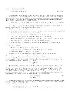
k FIG. 4: Shuffled lattice of the same kind of that in Fig. 3, but now with p(u) = (a/π)/(u2 + a2 ) where a = 1/50, i.e., with unlimited displacements and logarithmically diverging u. Again the agreement between the numerical simulation results and the theoretical prediction Eq. 27 is excellent. Note in particular that S(k) ∼ k at small k and that the remaining Bragg peaks, superimposed to the continuous contribution to the PS, are well modulated by weights proportional to |ˆ p(k)|2 with pˆ(k) = exp(−a|k|). Finally the PS at large k converges to average number density n0 = 1.

the PS of a spatially stationary stochastic process: ZZ dd xdd y e−i(k·x+q·y)C(x − y) = (2π)d δ(k + q)S(k) .

(28)

We also recall that by definition: D E n(x)n(y) = n20 + C(x − y) .

Furthermore, we define the functions fˆ(k1 , k2 ; x) and F (k1 , k2 ; q) respectively by the following FTs: ZZ fˆ(k1 , k2 ; x) = dd udd v e−i(k1 ·u+k2 ·v) f (u, v; x) ,

(29)

F (k1 , k2 ; q) =

Z

dd x e−iq·x fˆ(k1 , k2 ; x) .

(30)

The function fˆ(k1 , k2 ; x) is simply the characteristic function of the joint two-displacement PDF. By definition fˆ(k1 , k2 ; x) satisfies the following limit conditions fˆ(0, 0; x) = 1 for any x , and fˆ(0, k; x) = fˆ(k, 0; x) = pˆ(k) for any x > 0 .

10 By using Eq. 19 and Eqs. 28-30, we can write:   Z 1 d d q F (k, −k; q) + (31) S(k) = n0 1 − (2π)d Z
dd x e−ik·x fˆ(k, −k; x) n20 + Cin (x) − (2π)d n20 δ(k) .

R d 1 Note that (2π) d q F (k, −k; q) must be carefully hand dled. In fact, due to the properties of the inversion of the Fourier transform, it cannot be substituted directly by fˆ(k, −k; 0) if f (u, v; x) is discontinuous at x = 0 and continuous anywhere else as in the case of uncorrelated displacements presented above. Thus it must be understood as Z 1 (32) dd q F (k, −k; q) = lim fˆ(k, −k; x) . x→0 (2π)d More specifically, if f (u, v; x) is continuous at x = 0, i.e., lim f (u, v; x) = f (u, v; 0) ≡ δ(u − v)p(u) ,

x→0

then we have 1 (2π)d

Z

dd q F (k, −k; q) = 1 .

This condition is valid in all the cases in which the stochastic displacement field is a real continuous correlated stochastic process (see below the Gaussian example). In fact, in this case it is possible to prove a theorem [21] stating that the two-displacement correlation function is continuous everywhere, being equal to the onedisplacement variance u2 − u2 at x = 0. Instead, in the case of an uncorrelated stochastic displacement field this is no more true (it is not a continuous stochastic process), and, f (u, v; x) is discontinuous at x = 0 as shown by Eq. 21. This together with Eq. 32 gives for this case Z 1 2 dd q F (k, −k; q) = |˜ p(k)| . (2π)d With this prescriptions it is simple to recover Eq. 23 from Eq. 31 in the case of uncorrelated displacements. Instead, in the present case of a stationary correlated continuous stochastic displacement field, Eq. 31 can be rewritten as Z   S(k) = dd x e−ik·x fˆ(k, −k; x) n20 + Cin (x) − (2π)d n20 δ(k) ,

(33)

or equivalently S(k) = n20 F (k, −k; k) + (34) Z 1 dd q F (k, −k; q)Sin (k − q) − (2π)d n20 δ(k) . (2π)d Equations 33 can be further simplified by noticing that in the case of spatial statistical stationarity of both the

initial point-particle distribution and of the displacement field, the PS of the final particle distribution will not depend separately on the couple of displacements u and v applied at two points separated by the separation vector x, but on the relative displacement w = u − v. In fact let us call φ(w; x) the PDF that two points, separated by the separation vector x, perform a relative displacement w. By definition Z Z φ(w; x) = dd u dd v f (u, v; x) δ(w − u + v) . (35) If we take the FT of Eq. 35 with respect to w, we have ˆ x) = fˆ(k, −k; x) , φ(k; ˆ x) = F T [φ(w; x)]. Therefore Eq. 33 can be where φ(k; rewritten again Z   ˆ x) n2 + Cin (x) −(2π)d n2 δ(k) . S(k) = dd x e−ik·x φ(k; 0 0

(36) By using the PDF φ(w; x), Eq. 18 can be rewritten in a very intuitive form. This is done by noticing that for a generic stationary point process n(x) the quantity hn(x)n(y)i /n0 (where h...i is as usual the average over the considered ensemble of configurations n(x)) represents the average conditional density [25] of particles seen by a generic particle of the system at a separation x − y from it. By calling Γin (xE− y) = hnin (x)nin (y)i /n0 and D Γf (x − y) = n(x)n(y) /n0 the conditional densities respectively before and after the application of the displacement field, Eq. 18 transforms into: Z Γf (x) = dd x′ Γin (x′ ) φ(x − x′ ; x′ ) . Very often the CF is defined in a dimensionless way dividing C(x) by n20 , i.e., it is redefined as ξ(x) =

δ(x) C(x) = + h(x) , 2 n0 n0

which we call normalized covariance function (NCF). Consequently, also the PS is redefined as the FT of ξ(x): P (k) = F T [ξ(x)] =

S(k) 1 ˆ = + h(k) . n20 n0

It is simple to verify that if all the particles of the distribution have the same non-unitary mass m > 0, i.e., if P the microscopic mass density is ρ(x) = m n(x) = m i δ(x − xi ) with ρ0 = m n0 , the NCF ξ(x) of the microscopic mass density ρ(x) is equal to that of the microscopic number density n(x) and then is independent of m. For these rescaled quantities Eq. 36 can be rewritten as Z ˆ x) [1 + ξin (x)] − (2π)d δ(k) , P (k) = dd x e−ik·x φ(k;

(37)

11 It is important to note that, while ξin (x) depends on n0 at least through its diagonal part δ(x)/n0 , the twoˆ x), in our hydisplacement f (u, v; x), and therefore φ(k; pothesis, are in general supposed not to be (unless for particular choices of its momenta). Therefore, differently from the case of uncorrelated displacements, both Eqs. 33 and 35 can be divided into two parts, one dependent on n0 , and the other independent of it. This is a very important point because spatial distributions of particles with equal masses m are often used in numerical simulations as a discrete representation of continuous stochastic mass density fields. Consequently, in Eq. 33 and Eq. 35 there is a part depending on the discretization process and another part independent of it. This aspect is particularly important in the context of the gravitational n−body simulations in which, as above mentioned, the matter density field is usually represented, for numerical reasons, through a more or less dense distribution of particles with the same mass m [14] so that mn0 = ρ0 with ρ0 put equal to the average mass density of the continuous model. Small k expansion and large scale behavior - II

A.

Starting from Eq. 37, one can write a simple formula for the small k (i.e., large scale) behavior of the final PS of the particle distribution after the application of the displacement field. First of all let us study the small k ˆ x) = fˆ(k, −k; x). Since it is the FT behavior of φ(k; of φ(w; x), if Gµν (0) < +∞ (implying that the average value of w2 is finite at any x), we can write 2

ˆ x) = 1 − ik · w(x) − [k · w(x)] + o(k 2 ) , φ(k; 2

(38)

where w(x) is the relative displacement between two particles initially separated by a vector distance x. Let us suppose w(x) = 0 which is automatic in the case of statistical invariance for space inversion or any rotation (isotropy). Moreover, using the definition of Gµν (x) we can write 2

[k · w(x)] = 2

1,d X

k (µ) k (ν) [Gµν (0) − Gµν (x)] ,

µ,ν

where we have supposed also Gµν (x) = Gµν (−x). Using this expression and Eq. 38 in Eq. 37, we obtain at small enough k # " 1,d X (µ) (ν) k k Gµν (0) (39) P (k) ≃ Pin (k) 1 − µ,ν

+

1,d X µ,ν

k

(µ) (ν)

k



ˆ µν (k) + G

Z

 dd q ˆ Gµν (q)Pin (k − q) , (2π)d

ˆ µν (k) = F T [Gµν (x)] is the power spectrum mawhere G trix of the displacement field. Note that, since Gµν (0) =

R

dd q ˆ G (q), (2π)d µν

Eq. 39 can be also rewritten as:

P (k) ≃ Pin (k) +

1,d X µ,ν

+

Z

d

n ˆ µν (k) k (µ) k (ν) G

d q ˆ Gµν (q) [Pin (k − q) − Pin (k)] (2π)d



,

which is useful in particular in the case in which the initial particle configuration is the stationary Poisson one for which Pin (k) ≡ 1/n0 and the last term vanishes. Depending on the small k properties of Pin (k) and ˆ µν (k), the small k behavior of P (k) will change. Note G that Eq. 39 is valid only if Gµν (0) < +∞. In the case in which Gµν (0) = +∞ then the singular part of the small ˆ x) has to be considered in a similar k expansion of φ(k; way to the case of uncorrelated displacements given by Eqs. 24 and 25. A very particular and important case of Eq. 39 is given when perpendicular displacements are not correlated at any x. This means that Gµν (x) = δµν G(x) ˆ ˆ µν (k) = δµν G(k) (with δµν the Kronecher delta). and G ˆ If the displacement field is also isotropic, G(k) depends only on k (and consequently G(x) on x), so that the ˆ µν (k) is invariant under any PS matrix with elements G spatial rotation. In this case Eq. 39 can be rewritten as   (40) P (k) ≃ Pin (k) 1 − G(0)k 2   Z d d q ˆ ˆ + +k 2 G(k) G(q) Pin (k − q) (2π)d Similarly to Eq. 39, also Eq. 40 can be re-expressed as follows: n ˆ (41) P (k) ≃ Pin (k) + k 2 G(k)  Z dd q ˆ + G(q) [Pin (k − q) − Pin (k)] (2π)d Equations 40 and 41 are very useful because to show very clearly how effective a displacement field can be in “injecting” large scale correlations into a given particle distribution. As better clarified below, a central role is played by the spatial dimension d. Let us suppose that ˆ at small k we have Pin (k) ∼ k α and that G(k) ∼ k β (as already shown α, β > −d). Note that Z Z dd q ˆ G(q) Pin (k − q) = dd x e−ik·x G(x)ξin (x) , (2π)d and ξin (x) goes to zero at large x. Hence, when β < ˆ 0, in Eq. 40, the term k 2 G(k) is more effective than R dd q 2 ˆ k G(q)Pin (k − q) (i.e., the latter has an expo(2π)d nent larger than β + 2). For β = 0, apart from the R dd q ˆ very particular case in which (2π) d G(q)Pin (q) = 0, both terms are of the same order at small k, i.e., proportional to k 2 . Instead for β > 0, apart again the preˆ vious particular choices of G(k) in relation to Pin (k),

12 R dd q 2 ˆ ˆ prevails on k 2 G(k) ∼ k 2 (2π) d G(q)Pin (k − q) ∼ k β+2 k at sufficiently small k. We can therefore conclude that

Eq. 41 cancel one each other. We show this better in the following through the example of the Gaussian displacement field.

• β < 0: if α < β + 2 the displacement field is ineffective in changing large scale two-point correlations between particles. In fact the small k leading term of the final PS P (k) is the initial one Pin (k). For what concerns perturbations to this leading term, it is simple to show that, if α < β the main perturbation to the leading term due to the displacements is −G(0)k 2 Pin (k) ∼ k α+2 , while if β < α < β + 2 ˆ it is k 2 G(k) ∼ k β+2 (if α = β the two terms are of the same order).

Instead, if α > 2 again the small k behavior of the final PS is completely different from the initial one and is determined by the displacement field. In fact now the leading i term becomes h R dd q 2 ˆ ˆ k G(k) + (2π) ∼ k 2 . Howd G(q) Pin (k − q) ever the system after the action of the displacements is still in the superhomogeneous class of point processes in any d.

If instead α > β + 2, the displacement field completely determines the new large scale correlation properties of the particle distribution being ˆ k 2 G(k) ∼ k β+2 now the leading term of P (k). Since β > −d, the limit “most critical” behavior of P (k) which can be reached is k 2−d . Note that for d ≥ 3 long range non-integrable and mainly positive (i.e., critical) two-point correlations can be introduced in the system by the action only of displacements having finite variance G(0). Accordingly the (unreachable) limit decaying behavior for the NCF at large x is given by ξ(x) ∼ x−2 which is not integrable and long range. For example in d = 3 one can start from a completely uncorrelated Poisson particle distribution, and, applying finite displacements (i.e., with a finite average squared value) but with long range correlations, to obtain a particle distribution with a covariance function similar to those found at the critical point of a second order phase transition. For d ≤ 2 the exponent 2 − d ≥ 0, hence ξ(x) decays faster than x−d and correlations are not “critical”, but integrable (i.e., for our purpose, short range).

R dd q ˆ • β > 0. If (2π) d G(q)Pin (q) > 0, this case is similar to the case β = 0 with the difference that when α > 2 the main term introduced by the displaceR dd q 2 ˆ ment field is only k 2 (2π) d G(q) Pin (k − q) ∼ k . R dd q ˆ However if d G(q) Pin (q) = 0, which corre-

Finally, for −2 < β < 0 and α > β + 2 and any d, even though the leading term of P (k) is due to the displacement field which is characterized by long range correlations, the final particle distribution remains superhomogeneous (see Sec. II). • β = 0. If α < 2 the leading term of the final PS P (k) is again Pin (k). The displacement field introduces only higher order perturbations: (1) −G(0)Pin (k)k 2 ∼ ik α+2 , and (2) h R dd q 2 ˆ ˆ k G(k) + (2π) ∼ k 2 . The d G(q) Pin (k − q) former is the most important perturbative term for α < 0 (“critical” initial condition), while the latter is when 0 < α < 2. For α = 0 (1) and (2) are in general of the same order and both contribute to the main perturbation to Pin (k). However, if the initial particle configuration is a stationary Poisson one, Pin (k) ≡ 1/n0 for any k. Consequently, as shown explicitly by Eq. 41, the main perturbaˆ tion to Pin (k) is only k 2 G(k), as the other terms in

(2π)

sponds to a peculiar choice of the dependence of ˆ ˆ G(q) on Pin (q), the term k 2 G(k) can again be important. This case will be analyzed in more detail in the next section when the case of a shuffled lattice with correlated Gaussian displacements is analyzed. For the moment we notice only that this case is quite difficult to be realized because of the condition given by the Wiener-Khinchin theorem ˆ [22] which states that both Pin (k) and G(k) must be nonnegative at any k. This means that it can ˆ be realized only if Pin (k) is zero where G(k) is not and vice-versa, i.e., non-overlapping supports. Finally, note that when the initial particle configuration is a regular lattice, the term  Pin (k) 1 − G(0)k 2 in Eq. 40 is identically zero around k = 0. Consequently, the small k PS of the final configuration is determined by the next perturbation terms (see the next section about Gaussian displacements).

It is important to notice that Eqs. 39 and 40 are quite more complex than the result obtained in a naive way in Sec. III of the paper by simply using the continuity equation for the local conservation of mass which led basically to ˆ P (k) = k 2 G(k) . We see that respect to this simple approximation, even in the small k limit (i.e., large spatial scales) and finite displacements (i.e., finite G(0)), there can be important corrections coming both from the granularity of the system, from the internal correlations of the initial mass distribution, and from the interplay between these correlations and those of the displacement field.

13 VIII. CORRELATED GAUSSIAN DISPLACEMENT FIELD.

joint two-displacement PDF can be written as: 1 p × (43) 2 2π G (0) − G2 (x)   G(0)(u2 + v 2 ) − 2G(x)uv , exp − 2(G2 (0) − G2 (x))

f (u, v; x) = In this section the effect of a correlated displacement field on the correlation properties of a given particle distribution is further clarified through the discussion of a very important example: the Gaussian displacement field. Its importance is twofold: (1) its statistical properties are completely determined by the knowledge of one and two-point correlation functions (i.e., mean value u and correlation matrix Gµν (x)); (2) in many applications (e.g., initial conditions of cosmological n−body simulations) the Gaussian of perturbations (i.e., particle displacements) arises as a natural hypothesis basically due to arguments based on the central limit theorem [21]. Moreover, in order to clarify better all the concepts introduced in the previous section, two explicit examples of application of a Gaussian displacement field will be given: stationary Poissonian and regular lattice initial conditions. We treat in detail the particular case of a onedimensional spatially stationary point process nin (x) perturbed by a statistically stationary Gaussian displacement field u(x). The probability density functional Q[u(x)] giving the statistical weight of any realization u(x) of the field will have the form [25]:

where G(0) = u2 ≡ v 2 < +∞. It is also simple to verify that, in order to have this joint PDF well defined at all x, the correlation function G(x) must satisfy the following constraint: |G(x)| < G(0) ∀x 6= 0 . Note that if, as supposed, the Gaussian displacement field is a real continuous correlated stationary stochastic process and, consequently G(x) is a continuous function, then limx→0 G(x) = G(0). This implies then fˆ(k, −k; 0) = 1. If instead the displacement field is uncorrelated (i.e., G(x) = 0 for x 6= 0 but G(0) > 0), then, as shown in Sec. VI, fˆ(k, −k; 0) = exp[−k 2 G(0)] ≡ 2 |ˆ p(k)| with pˆ(k) = exp[−k 2 G(0)/2] being the characteristic function of the one-displacement PDF. In the case of truly continuous process, by taking the FT of Eq. 43 both in u and v, we find: ˆ x) = e−k2 (G(0)−G(x)) . fˆ(k, −k; x) ≡ φ(k;



Q[u(x)] ∼ exp −

1 2

ZZ

+∞

−∞

 dx dy u(x)K(x − y)u(y) ,

(42) where K(x) = K(−x) is the positive definite correlation kernel of the Gaussian displacement field. Without loss of generality we have put u = 0. Clearly Eq. 42 is only formal as, rigorously speaking, the normalization constant is infinite in the continuum space and also in the infinite volume limit. However we write it to make evident the meaning of Gaussianity for a stochastic field. For a more general account of Gaussian stochastic fields see [26, 30]. It is simple to show that the PS of the displacement field is given by ˆ G(k) =

1 . F T [K(x)]

Therefore, by using Eq. 44, the relation 33 between the PS of the particle distribution after the application of the displacement field, and its initial correlation function ξin (x) will be P (k) =

e−k

2

G(0)

G(x) ≡ u(x0 + x)u(x0 ) = F T −1



 1 , F T [K(x)]

which is a continuous function if u(x) is a continuous stochastic process [21]. It is possible to show that the

Z

+∞

dx e−ikx+k

2

G(x)

(1 + ξin (x)) −

−∞

2πδ(k) .

(45)

Since at large x both G(x) and ξin (x) converge to zero, the FT in x in Eq. 45 is not well defined and contains a Dirac delta function contribution exactly compensating the last Dirac delta function term in the same equation. This can be made more clear in the following way. The Dirac delta function of Eq. 45 can be transformed as: 2πδ(k) = 2πe

As we want u(x) to be a well defined continuous stochastic process, K(x) is to be taken so that the WienerKhinchin theorem is satisfied [21], i.e., K(x) is such that ˆ G(k) ≥ 0 at all k and integrable. The displacementdisplacement correlation function will be thus given by

(44)

−k2 G(0)

δ(k) = e

−k2 G(0)

Z

+∞

dx e−ikx .

−∞

Using this relation, Eq. 45 can be rewritten in the following form containing only well defined FTs: Z +∞  2  −k2 G(0) P (k) = e dx e−ikx ek G(x) − 1 + −∞

Z

+∞

−∞

dx e

−ikx+k2 G(x)

 ξin (x) .

(46)

The small k expansion of this formula can be obtained by simply applying to this case Eq. 40.

14 As already shown above, in d > 1 dimensions the more general form of f (u, v; x), even in the limited case of spatially stationary Gaussian displacement field is more complex. In fact in general not only parallel components of u and v can be correlated, but also perpendicular components can be. This leads to have a symmetric displacement-displacement correlation matrix Gµν (x). Once the correlation matrix is given, it is simple to show that, for a d−dimensional spatially stationary Gaussian displacement field with zero average value, we can write:

any d it is not possible to transform a Poisson particle distribution into a “superhomogeneous” one by the only action of the displacements. In fact, even though correlated, the displacements are stochastic perturbations and, consequently, cannot increase the level of large scale order of the system. B.

Shuffled lattice with correlated Gaussian displacements

In this subsection we analyze the effect of the same Gaussian displacement field as above on a one dimensional lattice (i.e., a regular chain of unit mass particles) with lattice spacing l (i.e., n0 = 1/l). Again we focus our attention on the large scales (k → 0 limit). By taking the inverse FT of Eq. 26, the initial NCF in this case is

ˆ x) ≡ fˆ(k, −k; x) = φ(k; " 1,d # X (µ) (ν) exp − k k [Gµν (0) − Gµν (x)] . µ,ν

However, in the case Gµν (x) = δµν G(x), the general features of the effect of a Gaussian displacement field can be well summarized by the above one-dimensional example.

A.

δ(x − nl) − 1 .

n=−∞

P (k) = le−k

In this section we analyze in detail the effect of a Gaussian displacement field as presented above on a onedimensional Poisson particle distribution. The extension to higher dimensions is straightforward. Let us suppose to have a spatially stationary Poisson particle distribution with constant average number density n0 > 0. As aforementioned in this case the NCF is δ(x) , n0

2

+∞ X

G(0)

e−iknl+k

2

G(nl)

− 2πδ(k) . (48)

n=−∞

The series in Eq. 48 is not well defined because its argument does not converge to zero for |n| → ∞. By using for 2πδ(k) the chain of identities " +∞ X  m −k2 G(0) 2πδ(k) ≡ 2πe × δ k − 2π l m=−∞  −∞,+∞ +∞  X X 2 m  e−iknl ≡ le−k G(0) × − δ k − 2π l n=−∞ m6=0

1 n0 .

By substituting this i.e., hin (x) = 0 and Pin (k) = initial NCF into Eq. 46, one finds: Z ∞   2 2 1 P (k) = + e−k G(0) dx e−ikx e−k G(x) − 1 , n0 −∞

−2πe−k

2

G(0)

×

−∞,+∞ X m6=0

 m , δ k − 2π l

we can rewrite Eq. 48 as P (k) = le−k

which, in the long wave-lengths limit, behaves as h i 1 ˆ − k 2 G(0) . + k 2 G(k) P (k) ≃ n0

+∞ X

Therefore Eq. 45 can be rewritten as

Gaussian displacement field applied to a Poisson particle distribution

ξin (x) =

ξin (x) = l

2

G(0)

+∞ X

n=−∞

(47)

ˆ Since in d = 1, G(k) ∼ k β with β > −1, we see that at small k the leading term is 1/n0 ≡ Pin (k) and the perturbations introduced by the displacements are at most of order k. However, as aforementioned, in d > 2 “critical” and dominating perturbations at small k can be introduced by the displacements. On the other hand, as clear from Eq. 47, we have a perturbation of order k 4 at small k due to the finite variance of the displacements G(0) which prevails on the perturbation coming from displacementdisplacement correlations (i.e., from the term containing ˆ G(k) in Eq. 47) if β > 2. We ultimately observe that for

+ 2πe−k

2

G(0)

−∞,+∞ X m6=0

h 2 i e−iknl ek G(nl) − 1

 m . δ k − 2π l

(49)

The first sum is a well defined series and gives in general the smooth part of P (k) converging to 1/n0 at large k. Instead the second one gives the singular delta-like Bragg peaks contribution to P (k) due to the initial perfect lattice distribution, each peak being modulated by 2 an amplitude e−k G(0) , rapidly decreasing to zero with increasing the position k of the peak. In d > 1 it is simple to obtain a very similar formula. Since this second contribution, due to the initial NCF, is exactly zero at all orders in the region −2π/l < k
0, and with α ≤ 0 then also G ˆ ˆ D (0) > 0 (but vanishing as then G(0) = 0, we can have G α k when l → 0) as the effect of the discretization of the Fourier transform. Another important observation about ˆ (2) (0) > 0. Eq. 50 is that, as [G(x)]2 ≥ 0 at all x, then G D Moreover, as [G(x)]2 decays faster than G(x) at large x ˆ D (0), is finite also G ˆ (2) (0) is. then, if G D

Simulation Theoretical

-2

P(k)

10

-4

10

-6

10

-2

-1

10

0

10

10

1

10

k FIG. 5: The figure presents the contribution to Eq. 49 coming from the first sum (i.e., excluding the delta-like Bragg peaks) to the PS P (k) of a 1d “shuffled lattice” obtained by applying a correlated Gaussian displacement field with ˆ G(k) = exp(−|k|/k0 ) with k0 = 1/4 (hence G(0) = u2 ≃ 0.08) to a regular chain of particles with unitary lattice spacing (l = 1). Both the theoretical prediction given by Eq. 49 and the numerical result obtained by a direct simulation with 104 particles are given. The agreement is excellent. Note that ˆ D (0) > 0 and finite we have that P (k) ∼ k2 since in this case G at sufficiently small k.

2π/l, the small k behavior of P (k) is completely determined by the first sum. This situation is very different from the case of an initial Poisson particle configuration. In fact, as shown above, in this second case the small k properties of the PS are determined mainly by the displacement field only if it produces “critical” large scale correlations (which is possible only in d > 2). Instead, in the present case, due to the particular properties of the lattice PS, it is always the displacement field to determine the large scale correlation properties, i.e., the small k PS. We now analyze in detail the small k behavior of P (k) in Eq. 49 with a particular attention to what kind of superhomogeneous distributions we can obtain after the application of the displacements. By keeping only the most important terms of Eq. 49 at small k, we can write: 4 ˆ D (k) + k [G ˆ (2) (k) − 2G(0)G ˆ D (k)] , k G 2 D (50) ˆ D (k) is the displus higher order terms. In Eq. 50 G cretized Fourier integral of G(x) with finite integration element given by the lattice cell size l, i.e.,

P (k) ≃ e−k

2

G(0) 2

ˆ D (k) = G

+∞ X

le−iknl G(nl) ,

n=−∞

and analogously ˆ (2) (k) = G D

+∞ X

n=−∞

le−iknl [G(nl)]2 .

(51)

These observations are very important in order to determine which kind of point processes can be realized by perturbing a lattice through a correlated stochastic displacement field. By the previous considerations, it is straightforward to see that the realization from a lattice of a stochastic particle distribution with P (k) ∼ k β at small k with β ≤ 2 (1 < β ≤ 2 in d = 1, and 2 − d < β ≤ 2 in general d dimensions) is a very simple task: it is enough to take a Gaussian displacement ˆ field such that G(k) ∼ k α with α = β − 2 ≤ 0 (see Figs. 5 and 6). Instead, obtaining a P (k) with β > 2 is a more difficult task. First of all one has to take a G(x) such that ˆ D (0) = 0. It is possible to see that this requirement is G a sort of stochastic expression of the total momentum conservation law in the system, that is, a conservation “in average” [29]. Moreover in order to have 2 < β < 4 ˆ D (k) ∼ k β−2 at small k. If instead one has to have G α ˆ GD (k) ∼ k with α ≥ 2 then β = 4 is obtained in all cases. The case β > 4 is not permitted. This means that, by perturbing a lattice with a (Gaussian) stochastic displacement field, the most “superhomogeneous” realizable point process has a PS P (k) ∼ k 4 at small k, e.g., k 6 is forbidden. This is a strong limitation. In fact, as aforementioned, from one side the PS of the lattice can be considered as behaving ∼ k ∞ around k = 0 (it is completely flat). From the other side we have just shown that an exponent β > 4 of P (k) is never realizable when one applies to any initial particle distribution a stochastic displacement field. This means that independently of the kind of the displacement field, as long as a smooth ˆ G(k) around k = 0 is considered, there is a “minimal level of disorder” injected in the system measured by the exponent 4 in the small k behavior of P (k). This shows how difficult is for example to build a spatially stationary stochastic point process such that P (k) ∼ k 6 at small k.

It is possible to extend all these results to higher dimension and to non-Gaussian displacement field, but we think that the example of the one-dimensional Gaussian displacement field is enough to enlighten the effects and the limitations of a general stochastic and correlated displacement field on a given point process statistically independent of it.

16 IX.

P(k)

1

CONCLUSIONS

simulation analytical result

0.01

0.0001 0.01

1

k FIG. 6: Power spectrum P (k) (including also the Bragg peaks contribution) of a shuffled lattice similar to the previous figˆ ure but now with G(k) = A exp(−k/kc )/(k + a) with kc = 5, a = 10−4 , and A = 1/20 (hence G(0) = u2 = 0.13). The agreement between the theoretical prediction and the numerˆ ical result is again excellent. Note that now, as G(k) ∼ k−1 at small k (but larger than a), the PS P (k) ∼ k in the same range.

FIG. 7: The figure presents a comparison between the PSs of (i) a Poisson point process, (ii) a shuffled lattice with uncorrelated displacements with a finite variance, and (iii) a shuffled lattice obtained by applying a correlated displacement field and showing a “critical” behavior at sufficiently small k. In particular all the particle distributions are in d = 1 and have the same mean density n0 (i.e., the same specific volume 1/n0 ). In the case (ii) the finite variance u2 < +∞ implies P (k) ∼ k2 at small k (see Eq. 23). Instead in (iii) the applied correlated displacement field for a ≪ k ≪ 2π/n0 has ˆ G(k) ∼ k−4 , and then, from Eq. 50, P (k) ∼ k2 . For k < a ˆ (which is below the minimal k of the figure) G(k) is cutoff to a constant value, in fact in any d the PS of any proper stochastic process has to satisfy limk→0 kd P (k) = 0.

In this paper we have discussed the effect of a stochastic displacement field on a spatial distribution of pointparticles with identical mass (i.e., point process) in the hypothesis of statistical independence between the two. In particular we have studied rigorously the changes induced in the two-point correlation properties of the particle distribution by the displacements. In this way we have seen that usual naive approaches to this problem leads to approximations (which may not be appropriate in some important cases) neglecting the contributions coming from either the initial correlation properties of the particle distribution or the failure of the small displacements approximation. We have distinguished the two cases of displacement fields with and without spatial correlations, giving for both cases the rigorous equations of transformation of the PS of the particle distribution. Our main interest concerns a detailed study of the kind of large scale correlations that the displacement field can “inject” into the system. In particular we are interested to know if long range positive spatial correlations in the system can be obtained by the application of a suitable displacement field to an initially short range correlated particle distribution. In this respect we have found that in d ≥ 3 it is possible to obtain particle distributions with long range correlations (i.e., with a covariance function with a positively diverging integral) by applying for instance either to a completely uncorrelated homogeneous Poisson point process or to a regular lattice of particles a Gaussian displacement field with sufficiently long range displacement-displacement correlations independently on the variance of the single displacement. This is a very important point, in fact we can think to perturb a lattice with such a displacement field with a mean squared displacement much smaller than the lattice spacing, and, independently of this, to obtain strong large scale typical fluctuations ∆N (R) of the number of points N (R) contained in a randomly placed sphere of radius R, growing as ∆N (R) ∼ Rα with α > d/2, whereas α = d/2 for the Poisson distribution and α = (d − 1)/2 for the regular lattice. Such particle distributions would look very similar respectively to the original Poisson or lattice particle distribution at the small scales (i.e., locally), but would show much larger (and more rapidly growing with the distance) fluctuations beyond a sufficiently large scale. Another related problem is to study how the long range order of a regular lattice array of particles is perturbed by the action of the applied displacement field. In particular we have studied between which limits the perturbed lattice stays in the so-called superhomogeneous class of point processes. That is, we have found the limits in which the sub-Poissonian character of the mass (i.e. the particles number) fluctuations on sufficiently large scales is conserved. Anyway we have also seen that any truly stochastic displacement field always injects into the particle system at least a minimal degree of disorder measured

17 by the α = 4 of the exponent of the final PS of the system P (k) ∼ k α at small k. We think that all these results can be of very practical importance in many physical and more largely scientific applications. For instance, this is the case of the so called n-body cosmological simulations. In this case the superposition of a suitable stochastic displacement field to a pre-initial particle distribution (e.g., a lattice of identical particles) is the usual way to prepare the initial conditions for numerical simulations to study the problem of the dynamic gravitational clustering of the matter leading to the formation of large scale structures (e.g., galaxies). These so built initial conditions should represent the spectrum of small primordial mass fluctuations predicted

by theoretical models (e.g., CDM models).

[1] J. M. Ziman, Principles of theory of solids 2nd ed., (Cambridge Univ. press, Cambridge, 1972). [2] N. W. Ashcroft and N. D. Mermin, Solid state physics, (Saunders College, 1976). [3] I. Groma, Phys. Rev. B, 56, 5807 (1997). [4] J.-P.. Hansen and I. R. McDonald, Theory of simple liquids, (Academic, New York, 1986). [5] C. Radin, Notices Amer.Math.Soc., 42, 26, (1995); Chapter in “Geometry at Work”, MAA Notes, 53 (Math. Assoc. Amar., Washington, DC, 2000). [6] P. J. E. Peebles, Principles Of Physical Cosmology, (Princeton University Press, 1993). [7] S. D. M. White, Lectures given at Les Houches astro-ph/9410043 (1993). [8] C. L. Chan and A. K. Katsaggelos, IEEE Transactions of Image Processing, 4, 743 (1995); C. Su and L. Anand, https://dspace.mit.edu/retrieve/3509/IMST015.pdf. [9] E. Renshaw, Biometrical Jour., 44, 718 (2002). [10] D. J. Daley and D. Vere-Jones, An introduction to the theory of point processes, (Springer Verlag, Berlin, 1988). [11] M. Kerscher, Phys. Rev. E, 64, 056109 (2001). [12] T. M. Truskett, S. Torquato, and P. G. Debenedetti, Phys. Rev. E, 58, 7369 (1998). [13] E. R. Harrison, Phys.Rev.D, 1, 2726 (1970); Ya. B. Zeldovich, Mon. Not. R. Acad. Soc., 160, 1, (1972). [14] G. Efstathiou, M. Davis, C. Frenk, and S. D. M. White, Astrophys. J. Supp. Series, 57, 241 (1985). [15] T. Baertschiger and F. Sylos Labini, Europhys. Lett., 57, 322 (2002). [16] P. Schneider and M. Bartelmann, Mon. Not. R. Astron. Soc., 273, 475 (1995). [17] Ya. B. Zeldovich, Astron. & Astrophys, 5, 84 (1970). [18] A. Gabrielli, M. Joyce, and F. Sylos Labini, Phys. Rev. D, 65, 083523 (2002). [19] A. Gabrielli, B. Jancovici, M. Joyce, J. L. Lebowitz, L. Pietronero, and F. Sylos Labini, Phys.Rev. D, 67, 043406,(2003). [20] T. Baertschiger, M. Joyce & F. Sylos Labini, Astrophys.

J. Lett., 581, L63 (2002). [21] B. Gnedenko, The theory of probability, (Mir Publishers, Moscow, 1975). [22] S. Torquato, Random Heterogeneous Materials, SpringerVerlag, Berlin, 2002). [23] A. Gabrielli and S. Torquato, in press on Phys. Rev. E; cond-mat/0405115. [24] S. Torquato and F. H. Stillinger, Phys. Rev. E, 68, 041113 (2003). [25] A. Gabrielli, F. Sylos Labini, M. Joyce, and L. Pietronero, Statistical Physics for Cosmic Structures, (Springer-Verlag Inc., Berlin, 2004). [26] C. W. Gardiner, Handbook of stochastic methods, (Springer Verlag, Berlin, Second Edition, 1997). [27] M. S. Bartlett, Jour. Roy. Stat. Soc., Ser. B Methodol., 25, 264 (1963). [28] W. Paul and J. Baschnagel, Stochastic processes from physics to finance (Springer-Verlag, Berlin, 1999). [29] A. Gabrielli, M. Joyce, B. Marcos, and P. Viot, Europhys. Lett., 66, 1 (2004). [30] R. J. Adler, The Geometry of Random Fields, (Wiley, London, 2001). [31] J. F. C. Kingman, Poisson processes, Oxford Studies in Probability, vol. 3, Clarendon Press, Oxford University Press (New York, 1993). MR 94a:60052 [32] O. Knill, Electronic Res. Announcements of the Am. Math. Soc., 3, 110 (1997). [33] In the case of ergodicity it can be taken also to be a volume average in the infinite volume limit. [34] E.g., the case in which p(u) = δ(u − u0 )/2 + δ(u + u0 )/2 for which pˆ(k) = cos(k · u0 ) and then |ˆ p(k)| = 1 for all k such that k · u0 = nπ with n any integer. [35] As |ˆ p(0)| = 1, for k = 0 instead we find singularly Sm (0) = Sin (0) at any m. This creates in general an asymptotic isolated discontinuity at k = 0. However this does not matter for the real space correlation properties as the Fourier transform of the PS is insensible to that.

X.

ACKNOWLEDGMENTS

The author thanks M. Joyce, F. Sylos Labini and L. Pietronero for discussions and continuous collaborations on related subjects. B. Marcos is warmly acknowledged for the fundamental help given in doing Figs. 3-6. The author thanks T. Baertschiger, S. Torquato and P. Viot for interesting discussions. Finally, the “E. Fermi” center of Rome (Italy) is also acknowledged.