Point spread functions and their applications to forensic image ...

FORENSIC SCIENCE JOURNAL SINCE 2002

Forensic Science Journal 2002;1:15-26

Point spread functions and their applications to forensic image restoration Che-Yen Wen,1,* Ph.D.; Chien-Hsiung Lee,1 B.S. 1

Department of Forensic Science, Central Police University, 56 Shu Jen Road, Taoyuan 333, Taiwan ROC.

Received: September 17, 2001/ Received in revised form: December 11, 2001 / Accepted: December 14, 2001

ABSTRACT In the forensic science field, there are many criminal image data including fingerprints, scene photos and surveillance camera videotapes. The evidence may become the key point to solve crimes. However, the evidence may be contaminated by the noise from crime scenes, or distorted by improper collecting procedures. In this case, the evidence will become void and we may lose the chance to arrest the criminals. The field of image restoration began primarily in the space programs of both the United States and the former Soviet Union in the 1950s and early 1960s. The image restoration technology was also extended to other fields, such as medical imaging and film media. Recently, some researchers tried to apply this technology to analyze data from the crime scenes. The ultimate goal of restoration techniques is to improve the quality of a degraded image. The degradation phenomena may come from motion blur, atmospheric turbulence blur, out-of-focus blur and electronic noises. In image restoration processing, we use point spread functions (PSF’s) to model these phenomena and restore degraded images with filters based on those PSF’s. However, in the forensic application, the case-dependent property of the PSF’s makes image restoration processing difficult. In this paper, we review several common PSF’s and apply them to solving image restoration problems. From the experimental results, we can obtain quality-improved images with proper PSF’s and filters. Keywords: Forensic image restoration, Point spread functions (PSF’s), Inverse filter, Wiener filter.

Introduction The major image processing technologies include restoration, enhancement, compression and recognition. For the application in forensic science, image restoration and image enhancement are frequently used. In this paper, we concentrate our attention on image restoration. The field of image restoration began primarily in the space programs of both the United States and the former Soviet Union in the 1950s and early 1960s [1]. The image restoration technology was also extended to other fields, such as medical imaging [2] and forensic science [3]. The ultimate goal of restoration techniques is to improve the quality of a degraded image. The degradation phenomena may come from motion blur, atmospheric turbulence blur, out-of-focus blur and electronic noises. In practice, we consider image restoration to be a process that attempts to reconstruct or recover a degraded image by using knowledge of the causes of the degradation phenomena. Thus restoration techniques are oriented toward mathematically modeling the degradation (point spread functions, PSF’s) and applying the inverse process to recover the original image [1,4,5]. * Corresponding author, e-mail:[email protected]

In the forensic science field, there are many criminal data including fingerprints, scene photos and surveillance camera videotapes. The evidence may become the key point to solve crimes. However, the evidence may be contaminated by the noise from crime scenes, or distorted by improper collection. In this paper, we model this contamination with PSF’s including 1-D motion blur, 2D motion blur, 1-D Gaussian blur, atmospheric turbulence blur, and uniform out-of-focus blur. We apply the filters (the inverse filter and the Wiener filter) based on these PSF’s to image restoration and use synthetic images to assess their capability.

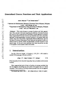
Methods The degradation process can be modeled as in Fig.1.

Fig. 1 The image degradation process, f (m,n) is an original image, H is a specific PSF that degrades the original image, n(m,n) is an additive noise term, and g(m,n) is the degraded (or observed) image.

16 Forensic Science Journal 2002; Vol. 1, No. 1 f(m,n) is an original image (where m and n are coordinates of a point on an image, the value of f(m,n) is the intensity or the gray-level value of the point), H is a specific PSF that degrades the original image, n(m,n) is an additive noise term, and g(m,n) is the degraded (or observed) image. Their relationship can be described as (1) The digital image restoration may be viewed as the process of estimating (the approximation of f(m,n)), given g(m,n) and n(m,n) [1]. Unfortunately, it is not easy for us to know the exact degradation models. In practice, we obtain the models by experimental estimation or statistical characteristics [6]. Any available information (observed images and the devices used to acquire images) and the expert’s experience can be applied to solve the specific application. A general block diagram for the images restoration process is provided in Fig. 2. The development of the degradation model is based on degraded (observed) images and the knowledge of the image formation process. The knowledge of the image formation process is the information about how a specific lens distorts an image or how the camera-shaking motion affects an image. This kind of information can be provided by the image-capture process, or be extracted from the degraded images by image analysis techniques. The inverse degradation process can be derived from the degradation model, and it can be applied to restoring the degraded image g(m,n). After the inverse degradation process, we can obtain the restored or estimated image . is the restored image that represents an estimate of the original image f(m,n). This process is repeated until satisfactory results are achieved. We can treat the image restoration as the procedures of finding an approximation to the degradation process and finding the appropriate inverse process to estimate the original image [7]. In the space domain, a degraded image g(m,n) is created via an original image f(m,n) convolving with the linear operator h(m,n) of the degradation system. It is defined as

Fig. 2 The concept of the image restoration process [7].

(spatial domain),

(2)

where “*” denotes the convolving operator. The representation in the frequency domain is (frequency domain),

(3)

where G(u,v), H(u,v) and F(u,v), and are the Fourier transforms of g(m,n), h(m,n) and f(m,n), respectively. In the terminology of linear system theory, H(u,v) is called the transfer function of the system. In optics, H(u,v) is called the optical transfer function (OTF), and its magnitude is called the modulation transfer function [8]. In order to introduce the point spread function (PSF), the Fourier transform of the OTF, we suppose h(m,n) is unknown and apply a unit impulse function (i.e. a point of light) to the system; the Fourier transform of a unit impulse is simply 1, from Eq.(3), G(u,v)=H(u,v). The inverse transform of the output G(u,v) becomes h(m,n). This result comes from well known linear system theory [6,8,9]: A linear position invariant (LPI) system is completely specified by its response to an impulse. When the Fourier transform of a unit impulse is applied to such a system, its output is precisely the system transfer function H(u,v). Alternatively, applying the impulse directly yields h(m,n) at the output, that is, the system output is the convolution of the system input and the system’s impulse response. For this reason, h(m,n), the inverse transform of the system transfer function, is called the impulse response in the terminology of linear system theory. In optics, h(m,n), the inverse of the optical transfer function, is called the point spread function (PSF). This name is based on the optical phenomenon that the impulse corresponds to a point of light and that an optical system responds by blurring (spreading) the point, with the degree of blurring being determined by the quality of the optical components. Thus the OTF and the PSF of a linear system form a Fourier transform pair. In practice, the PSF h(m,n) and the noise n(m,n) may be obtained by estimation and experiments. Point Spread Functions (PSF’s) We describe the point spread function (PSF) as h(m,n), which is the 2D impulse response produced from a point source of light passing through the degradation system in the absence of noise. Although we have the method to estimate the PSF’s (such as defocus, camera shaking, object motion, etc.), in practical forensic image restoration, it is not easy for us to obtain the exact parameters of PSF’s. That is because the real degradation may come from several PSF’s simultaneously. What we often do is to choose one or several “proper” PSF models from what we have so far. Those PSF’s include 1-D motion blur, uniform 2-D motion blur, Gaussian blur,

Wen et al.: Point spread function 17

atmospheric turbulence blur, and uniform out-of-focus blur [1,10]. We summarize them as follows: 1. 1-D motion blur: This model is suitable for one dimension camera panning or fast object motion; the equation is described as

(4) where L is the moving distance. 2. Uniform 2-D motion blur: This model is used to describe the motion of camera or object in two dimensions, (5) where L is the moving distance. 3. Gaussian blur: This model is a blur model based on the Gaussion distribution model, (6) where σ 2 is the variance that determines the severity of the blur. 4. Atmospheric turbulence blur: This model is often applied to remote sensing and aerial images whose blur effect is due to long-term exposure. Actually, it is also a 2-D Gaussian blur model, (7) where K is a constant, and σ 2 is the variance that determines the severity of the blur. 5. Uniform out-of-focus blur: Defocus of photography can often be found in many photo images. This type of blur is primarily due to the following factors: the focal length, the camera aperture size and shape, the distance between object and camera, the wavelength of the incoming light, and the effects due to diffraction. It is difficult to obtain all of these parameters after a picture has been taken; however, we can use the uniform out-offocus model as an approximation of the PSF,

Restoration Filters The goal of the image restoration technologies is to estimate an original image f from g, H and (see Fig.1). Based on Eq.(1), we can obtain the estimated original image by a linear algebraic approach. The key concept of the linear algebraic approach is to seek (an estimate of f ) by minimizing the difference between f and . Based on the five PSF’s, we apply the Inverse filter and the Wiener filter to restore degraded images. 1. Inverse Filter The Inverse filter is a straightforward image restoration method. If we know the exact PSF model in the image degradation system and ignore the noise effect, we can restore the degraded images based on Eqs. (2) and (3). In practice, the PSF models of the blurred images are usually unknown and the degraded process is also affected by the noise, so the restoration result with the Inverse filter is not usually perfect. However, since this method is simple, we suggest this filter as the first step in solving forensic image restoration cases. From Eq.(1), we can obtain n=g-H f. If we want to ignore n and use to let H approximate it under the least square sense, we can obtain the error function, (10) Since we require the minimum of the J( ), and is not constrained in any other way, this linear algebra is called an unconstrained restoration. In order to minimize the value of J( ), we differentiate J( ) with respect to J( ) and let the result be equal to the zero vector, i.e. (11) where the superscript T means the transpose matrix. We solve Eq.(11) for and obtain (12) The Fourier transform of Eq.(12) is (13)

(8) From Eq.(13) and its inverse Fourier transform -1 ℑ ( ), we can obtain the restored image ,

where R is the circular radius of defocus blur. (9)

(14)

The above models can appear in a single term like Eq.(2), or in a compound term. Based on the LPI assumption, we can obtain the compound PSF models as [10] where “*” is the convolving operator.

When we apply Eq.(13) to restore images, we may meet a mathematical puzzle–division by zero. Even as the values in H(u,v) become very small, we will have very large values in . The above situations will cause a computing problem. One method to deal with this

18 Forensic Science Journal 2002; Vol. 1, No. 1 problem is to limit the restoration to a specific radius about the origin on the spectrum plane. That is, we can use the restoration cutoff frequency to avoid small values of H(u,v). In practice, the selection of the cutoff frequency must be experimentally determined [7]. 2. Wiener Filter When considering the noise effect, we will use the Wiener filter. In stead of using Eq.(10), we rewrite the criterion equation as [10]

(15) where Q is a linear operator on and is a constant called the Lagrange multiplier. Again, we differentiate Eq. (15) with respect to and set the result equal to the zero vector,

Eq.(20) can be considered as the standard Wiener filter; otherwise, Eq.(20) is called the parametric Wiener filter (PWF). 2. Type II: When absence of noise, i.e. Sη(u,v) = 0, the Eq.(20) becomes the Inverse filter (see section 2.2.1). 3. Type III: If Sη(u,v) and Sf (u,v) is unknown, we can rewrite Eq.(20) as (21)

where K is the ratio of noise power spectrum to the original image power spectrum and is considered as a constant. The optimal K value must be experimentally determined. If K > H(u,v),

(16) We solve Eq.(16) for

, it means the restoration of degraded images is not influenced by the additive noise [6,7].

and obtain (17)

where γ = 1/α. The Fourier transform of Eq. (17) is (18) where u = 0,1,2......,M-1, v = 0,1,2,.....N-1, γ = 1/α, S η = N(u,v) 2  = power spectrum of the noise, S f = F(u,v)2 = power spectrum of the original image, H*(u,v) is the complex conjugate of H(u,v) in the frequency domain, (19)

Experimental Results In this paper, we will use two synthetic images, lena (Fig.3) and vehicle number plate(Fig.21), to compare the restoration results of the Inverse filter and the Wiener filter, based on the five PSF models. Then, we will show a real forensic case solved by the image restoration technology. Synthetic Lena image test We applied the five PSF’s to blur the original lena image (Fig.3), then we used the Inverse filter and the Wiener filter to restore the blurred image. 1. Inverse filter: (see Fig. 4~8)

We can rewrite Eq. (18) as Eq. (20),

(20) where γ [Sη(u,v)/Sf (u,v)] denotes the power spectrum ratio. We call the outer square bracket term in Eq.(20) as the power spectrum ratio Wiener filter (PSRWF). With Eq.(20), we can apply it to image restoration problems in three situations: 1. Type I: If γ = 1, the right item (PSRWF) in

Fig. 3 The synthetic lena image, image size = 256 × 256.

Wen et al.: Point spread function 19

(a)1-D motion blur:

(c)1-D Gaussian Blur:

(a)

(a)

(b)

(b)

Fig. 4 (a) the 1-D motion blurred image of “lena”;(b) the restored image with the inverse filter.

(b)Uniform 2-D motion blur:

(a)

(b)

Fig. 5 (a)the uniform 2-D motion blurred image of “lena”; (b)the restored image with the inverse filter.

Fig. 6 (a) the 1-D Gaussian blurred image of “lena”; (b) the restored image with the inverse filter.

(d)Atmospheric turbulence blur (or 2-D Gaussian blur): (a)

(b)

Fig. 7 (a) the 2-D Gaussian blurred image of “lena”; (b) the restored image with the inverse filter.

20 Forensic Science Journal 2002; Vol. 1, No. 1 (e)Uniform out-of-focus blur: (a)

(b)

Fig. 8 (a) the uniform out-of-focus blurred image of “lena”; (b) the restored image with the inverse filter.

2. Wiener filter Besides the PSF degradation, we add some noise (with the uniform distribution) to the original lena image and do the experiments again with two types of the Wiener filter: A. Type I : Eq.(20) with Sη = N(u,v)2, Sf = F(u,v)2 and γ = 1. B. Type III: Eq.(21) with different K values. (a)1-D motion blur: (Fig. 9,10) A. (a)

(b)

Fig. 9 (a) the 1-D motion blurred image of “lena”; (b) the restored image with the Type I Wiener filter.

B.

Fig. 10 (a) ~ (h) are the restored results of the 1-D motion blurred “lena” images with the Type III Wiener filter of different values of K. From the above figures, we get the best restoration result when K=10-2.

Wen et al.: Point spread function 21

(b)Uniform 2-D motion blur: (Fig. 11, 12)

(c)1-D Gaussian blur: (Fig. 13~15)

A.

A.

(a)

(a)

(b)

(b)

Fig. 11 (a) the uniform 2-D motion blurred image of “lena”; (b) the restored image with the Type I Wiener filter.

Fig. 13 (a) the 1-D Gaussian blurred image of “lena”; (b) the restored image with the Type I Wiener filter.

B.

Fig. 12 (a) ~ (h) are the restored results of the uniform 2-D motion blurred “lena” images with the Type III Wiener filter of different values of K. From the above figures, we get the best restoration result when K = 10-2.

22 Forensic Science Journal 2002; Vol. 1, No. 1 B.

Fig. 14 (a) ~ (h) are the restored results of the 1-D Gaussian blurred “lena” images with the Type III Wiener filter of different values of K. From the above figures, we get the best restoration result when K = 103.

We enlarge the sub-regions of Fig.14, and obtain more details as Fig. 15.

Fig. 15 (a) ~ (d) are the detail images of Fig. 14. (d), (e), (g), and (h) respectively.

(d) Atmospheric turbulence blur or 2-D Gaussian blur: (Fig. 16~18) A. (a)

(b)

Fig. 16 (a) the 2-D Gaussian blurred image of “lena”; (b) the restored image with the Type I Wiener filter.

Wen et al.: Point spread function 23

B.

Fig. 17 (a) ~ (h) are the restored results of the 2-D Gaussian blurred “lena” images with the Type III Wiener filter of different values of K. From the above figures, we get the best restoration result when K = 102~103.

We enlarge the sub-regions of Fig.17, and obtain more details as Fig.18.

Fig. 18 (a) ~ (d) are the detail imges of Fig. 17. (c), (d), (f), (h) respectively.

(e)Uniform out-of-focus blur: (Fig. 19~20) A. (a)

(b)

Fig. 19 (a) the uniform out-of-focus blurred image of “lena”; (b) the restored image with the Type I Wiener filter.

24 Forensic Science Journal 2002; Vol. 1, No. 1 B.

Fig. 20 (a), (c), (d) are the restored images of the uniform out-of-focus blurred “lena” images with Type III Wiener filter when k is equal to 1, 10, and 100 respectively; (b) the detail image of (a).From the experimental results, we get similar restoration results when 0 < K ≤ 1.

From above experiments, we find the restoration results with the Type I Wiener filter (A) are better than those with the Type III Wiener filter (B), since the noise and image energy are known exactly. However, in practical applications, it is difficult for us to obtain the energy information. That is why we use the PSRWF (Type III) frequently.

2. Wiener filter (a)1-D motion blur: A.

(a)

Synthetic vehicle number plate test

(b)

Fig. 24 (a) the 1-D motion blurred image of “vehicle plate”; (b) the restored image with the Type I Wiener filter.

In this section, we use a synthetic vehicle number plate (the vehicle No. “CA-6401”, image size = 256 × 128, see Fig.21) to compare the restoration results of the Inverse filter and the Wiener filter. Since the results are similar to previous lena image experiments, we just show the experimental results of 1-D motion blur and Uniform 2-D motion blur models.

B.

Fig. 21 The synthetic vehicle number plate image, image size = 256 × 128.

1. Inverse filter (a)1-D motion blur:

(a)

(b)

Fig. 22 (a) the 1-D motion blurred image of “vehicle plate”; (b)the restored image with the inverse filter.

Fig. 25 (a) ~ (h) are the restored results of the 1-D motion blurred “vehicle plate” images with the Type III Wiener filter of different values of K. From the above figures, we get the best restoration result when K = 10-5.

(b)Uniform 2-D motion blur:

(b)Uniform 2-D motion blur A.

(a)

(b)

Fig. 23 (a)the uniform 2-D motion blurred image of “vehicle plate”; (b)the restored image with the inverse filter.

(a)

(b)

Fig. 26 (a) the uniform 2-D motion blurred image of “vehicle plate”; (b) the restored image with the Type I Wiener filter.

Wen et al.: Point spread function 25

B.

Fig. 27 (a) ~ (h) are the restored results of the uniform 2-D motion blurred “vehicle plate”images with the Type III Wiener filter of different values of K. From the above figures, we get the best restoration result when K = 10-5.

From the above experiments, we obtained similar results as in the previous lena image test. Real vehicle plate number test In this section, we apply the digital restoration technology to a vehicle plate number image from a real forensic case. The image is shown in Fig. 28.

Fig. 30 The enlarged image.

(a)

(b)

Fig. 28 (a)The vehicle plate number image from a real forensic case; (b)The sub-image with plate numbers.

We apply the Inverse filter with the 2-D Gaussian blur PSF model to the plate number sub-image (Fig.28(b)) and obtain the restored image (Fig.29).

Fig. 31 The last vehicle plate number in Fig.30.

(a)

(b)

(c)

(d)

(e)

(f)

(g)

(h)

(i)

(j)

Fig. 29 The restored image with the Inverse filter.

We enlarge the Fig.29 image and obtain Fig.30. We check the enlarged image and find the last number has the greatest chance for successful restoration, so we just concentrate on the last number as Fig.31.

Fig. 32 The known vehicle plate number patterns.

26 Forensic Science Journal 2002; Vol. 1, No. 1 Finally, we enhance Fig.31 and compare it to the known vehicle plate number patterns (we made them in advance, see Fig.32). From human visual inspection, we find the restored number image is 2 (see Fig.33). When this case was solved, we obtained the image of the original vehicle plate numbers, and show it in Fig.34 for comparison.

models and the restoration approaches–the Inverse filter and the Wiener Filter. We compare the performance with the synthetic lena and vehicle number plate images. Then, we show a real case solved by the restoration technique. Because the noise effect in the real case is not serious, the restoration results by using the inverse filter and the Wiener filter are similar. In practical applications, since the parameters of the degraded processes are not easy to be obtained exactly, we suggest the first step is trying the Inverse filter, since it is simple. In future work, we will try to compare the observed (blurred) images with the ideal distorted digits (by known PSF’s), and see if we can obtain better recognition.

References (a)

(b)

Fig. 33 (a) the restored number image;(b) the known vehicle plate number pattern,2.

Fig. 34 The image of the original vehicle plate numbers; this photo was taken after the case was solved.

Conclusions The ultimate goal of the restoration techniques is to improve the visual-quality of a degraded image. In this paper, we focus on the discussion of the degradation

1. Banham MR., Katsaggelos AK. Digital Image Restoration. IEEE Signal Processing Magazine. 1997 Mar; 14(2):24-41. 2. Chan CL, Katsaggelos AK, Sahakian AV. Image Sequence Filtering in Quantum -Limited Noise with Applications to Low-Dose Fluoroscopy. IEEE Trans. Medical Imaging. 1993 Sep;23:610-21. 3. Raymond Hsieh, Digital Images Restoration and its applications in forensic science (Chinese) 2000 Mar; 49:115-32. 4. Andrews HC, Hunt BR. Digital Image Restoration. Englewood Cliffs: NJ: Prentice-Hall. 1977. 5. Angwin DL, Kaufman H. Digital Image Restoration. New York: Springer-Verlag. 1991. 6. Gonzalez RC, Woods RE. Digital Image Processing. Addison-Wesley Company. 1992. 7. Umbaugh SE. Computer Vision and Image Processing. Prentice-Hall, 1998;151-96. 8. Lee HC. Review of image-blur models in a photographic system using the principles of optics. Optical Engineering.1990 May;29(5):405-21. 9. Meinel E. Origins of Linear and Nonlinear Recursive Restoration Algorithms. Journal Optical Soc.Amer. 1986 June;13:787-99. 10. Schowengerdt RA. Remote Sensing Model and Method for Image Processing. 2nd ed. Academic Press.1997:77-83.