construct design of experiments (DOEs) to minimize the maximal RMS bias errors or compare different DOEs. It is demonstrated that for high dimensional design ...
AIAA 2006-724
44th AIAA Aerospace Sciences Meeting and Exhibit 9 - 12 January 2006, Reno, Nevada
Pointwise RMS bias error estimates for design of experiments Tushar Goel*, Raphael T. Haftka† Department of Mechanical and Aerospace Engineering, University of Florida, Gainesville, FL 32611 Wei Shyy‡ Department of Aerospace Engineering, University of Michigan, Ann Arbor, MI 48109 Layne T Watson§ Department of Computer Science and Mathematics, Virginia Polytechnic Institute, Blacksburg, VA 24061 Abstract Response surface approximations offer an effective way to solve complex problems. However limitations on computational expense pose restrictions to generate ample data and a simple model is typically used for approximation leaving the possibility of errors due to insufficient model known as bias errors. This paper presents a method to estimate pointwise RMS bias errors in response surface models. Prior to generation of data, RMS bias error estimates can be used to construct design of experiments (DOEs) to minimize the maximal RMS bias errors or compare different DOEs. It is demonstrated that for high dimensional design spaces, central composite design gives a reasonable trade-off between variance and bias errors under conventional assumption of quadratic model and cubic true function. The results indicate that compared to bounds on bias error, RMS estimates are less affected by increase in the dimensionality of the problem. Latin Hypercube Sampling (LHS), though very popular, may yield large unsampled regions which can be successfully detected by implementing an alternate criterion like maximum standard error or maximum RMS bias error in design space. We further demonstrate that poor LHS designs can be eliminated by using more than one DOE. With the help of a non-polynomial example problem, it is demonstrated that the proposed method is correctly able to identify the regions of high errors even when assumed true model is not accurate.
I.
NOMENCLATURE
A b c l, c u DOE E(x) e e(x)
Alias matrix Vector of estimated coefficients of basis functions Vectors of bounds on the coefficients vector β Design of experiment Expected value of x Vector of true errors at the data points Error at design point x
rms e act ( x)
Actual RMS error at design point x
e brms ( x)
RMS bias error at design point x
e bI ( x)
Data independent bias error bound at design point x
eb(x)
True bias error at design point x
*
Graduate Student, Student Member AIAA Distinguished Professor and Fellow AIAA ‡ Clarence L “Kelly” Johnson Collegiate Professor and Fellow AIAA § Professor †
American Institute of Aeronautics and Astronautics
Copyright © 2006 by the paper authors. Published by the American Institute of Aeronautics and Astronautics, Inc., with permission.
1
ees(x) f(x), f(1)(x), f(2)(x) fj(x) N(µ,σ) NP Ns Nv n1 n2 r V X, X(1), X(2) x x1, x2, …,xn x1(i), x2(i),…, xn(i) y y(x) ŷ(x) α1, α2, …, αm
Estimated standard error at the design point x Vectors of basis functions at x Basis functions Normal distribution with mean µ and standard deviation σ Number of true candidate polynomials Number of design data points Number of design variables Number of basis functions in the regression model Number of missing basis functions in the regression model Parameter used to construct DOEs Design space Gramian (Design) matrices Design point (vector) Design variables Design variables for ith design point Vector of observed responses Observed response at design point x Response surface approximation at a design point x Parameters used to construct DOEs
β, β (1) , β ( 2) βj, βj(1), βj(2)
Vectors of basis function coefficients Coefficients of basis functions
γ
Bound on coefficient vector β Noise in the response True mean response at x Parameter used to construct DOEs Noise variance Root mean square (rms) error Maximum value of the quantity over the design space Space averaged value of the quantity An instance of a true polynomial
( 2)
ε
η(x) θ
σ2 σa ()max ()avg Subscript c
II.
INTRODUCTION AND LITERATURE REVIEW
Polynomial response surface approximations (RSAs) are widely adopted for solving optimization problems with high computational or experimental cost, as they offer a computationally less expensive way of evaluating designs. It is important to ensure the accuracy of RSAs before using it for design and optimization. The accuracy of RSA, constructed using a limited number of simulations, is primarily affected by two factors: (i) noise in the data; and (ii) inadequacy of the fitting model (called modeling error or bias error). In experiments noise may appear due to measurement errors and other experimental errors. Numerical noise in computer simulations is usually small, but it can be high if there are some unconverged solutions such as those encountered in CFD or structural optimization. The true model representing the data is rarely known and due to limitation on the amount of data available, usually a simple model is fitted to the data. For simulation-based RSAs, modeling/bias error is mainly responsible for the error in prediction. The effect of different errors can be reduced by careful sampling of the points using design of experiment techniques. There are two considerations for a good design of experiment: (i) dominant source of error in experiment and (ii) uniformity (called stability by Myers and Montgomery [1]) over the design space (small variation of error in design space). When noise is the dominant source of error, there are a number of experiments which minimize the effect of variance (noise) on the resulting approximation, for example, the central composite (Box and Wilson, [2]) and the Box-Behnken designs for regularly shaped design spaces and, the D-optimal design (Myers and Montgomery [1], chapters 7 and 8) which minimizes the variance associated with the estimates of coefficients of response surface model for irregularly shaped design spaces. Traditional variance-based designs minimize the effect of noise and attempt to obtain uniformity (stability) over design space but they do not address bias errors. Recently Goel et al. [3] have demonstrated that prediction variance is not an appropriate tool to estimate errors when bias errors are dominant. American Institute of Aeronautics and Astronautics
2
It is more difficult to achieve uniformity when bias errors are dominant. Traditional minimum bias designs consider only integrated error measures (Myers and Montegomery [1]) in design of experiments. A good amount of work has been done on developing design of experiments which minimize mean squared errors averaged over the design space that combines variance and bias errors (averaged or integrated mean squared error) [4–7]. The bias component of the averaged or integrated mean squared error was also minimized to obtain so-called minimum bias designs. The fundamentals of minimizing integrated mean squared error and its components can be found in Myers and Montgomery [1] (chapter 9) and Khuri and Cornell [8] (chapter 6). Venter and Haftka [9] developed an algorithm implementing a minimum-bias criterion, necessary for an irregularly shaped design space where no closed form solution exists for minimum-bias experimental design. They compared minimum-bias and D-optimal experimental designs for two problems with two and three variables. The minimum-bias experimental design was found to be more accurate than D-optimal for average error but not for maximum error. Montepiedra and Fedorov [10] investigated experimental designs minimizing the bias component of the integrated mean square error subject to a constraint on the variance component or vice versa. Fedorov et al. [11] later studied design of experiments via weighted regression prioritizing regions where the approximation is desired to predict the response. Their approach considered both variance and bias components of the estimation error. Palmer and Tsui [12] studied minimum-bias Latin hypercube experimental design for sampling from deterministic process simulators. Qu et al. [13] implemented Gaussian quadrature-based minimum bias design and presented minimum bias central composite designs for up to six variables. Since minimum-bias designs do not achieve uniformity, designs that distribute points uniformly in design space (space filling designs like Latin-Hypercube Sampling) are popular even though these designs have no claim to optimality. However due to random component these designs occasionally can leave large holes in design space which may lead to poor predictions. Bias error averaged over the design space has been studied extensively but there is relatively small amount of work done to account for pointwise variation of bias errors because of inherent difficulties. Pointwise error estimates are useful to identify regions of large errors and to reduce the maximal absolute bias error rather than the spaceaveraged error. An approach for estimating pointwise bounds on bias errors in RSAs following the pointwise decomposition of the mean squared error into variance and the square of bias was developed by Papila and Haftka [14]. They used the bounds to obtain design of experiments that minimize the maximum absolute bias error. Papila et al. [15] extended the approach to account for the data and proposed data-dependent bounds. They assumed that the true model is a higher degree polynomial than the approximating polynomial and it satisfies the given data exactly. Goel et al. [3] generalized this bias error bounds estimation method to account for inconsistencies between the assumed true model and actual data, and rank deficiencies in the matrix of equations used in linear regression. They demonstrated that the bounds can be used to develop adaptive design of experiment to reduce the effect of bias errors in region of interest. For high dimensional problems due to increase in number of coefficients not modeled by response surface model, bias error bound estimates pose two main problems: (i) computational cost of estimating bounds by solving optimization problem increases (polynomial growth rate with increase in number of variables in optimization problem), and (ii) the practical utility of error bounds diminishes as the probability of occurrence of the error predicted by bounds becomes very small (refer to Appendix A for demonstration). To address these two issues, a method to estimate pointwise root mean square (RMS) bias errors (instead of bounds) is proposed in this work. The RMS bias error estimates can be used as a possible metric to construct DOEs or to compare different design of experiments. The paper is organized as follows: The next section presents the theoretical formulation of the pointwise RMS bias error estimation method. Different error metrics to construct and compare DOEs are also given. Major results of this study are given in Section 4. Specifically, the RMS bias error estimates are used to construct and compare different design of experiments for a quadratic response surface when assumed true model is cubic. One nonpolynomial example involving multiple sinusoidal inputs of different wave lengths was used to study the application of RMS bias errors when assumed true model was incorrect. Conclusions and issues identified are summarized in Section 5.
III.
THEORETICAL MODEL FOR ESTIMATING POINTWISE RMS BIAS ERRORS T
Let the true response η(x) at a design point x be represented by a polynomial f (x)β , where f(x) is the vector of basis functions and
β is the vector of coefficients. The vector f(x) has two components: f (1) (x) is the vector of
basis functions used in RSA or fitting model, and f
(2)
(x) is the vector of additional basis functions which are
American Institute of Aeronautics and Astronautics
3
missing in the linear regression model. Similarly, the coefficient vector β can be written as a combination of vectors
β (1) and β ( 2) which represent the true coefficients associated with the basis function vectors f (1) (x) and f (2) (x) respectively. That is:
η ( x) = f (x)β = f T
(1 ) T
f
( 2 )T
β (1 ) ( 2 ) = (f (1) (x)) T β (1) + (f ( 2 ) ( x)) T β ( 2 ) β
(1)
Assuming normally distributed noise ε with zero mean and variance σ ( N (0, σ ) ), the observed response y(x) at a design point x is given as 2
y ( x) = η ( x) + ε
(2)
The predicted response at a design point x, yˆ ( x) is given as a linear combination of approximating basis functions vector f
(1)
( x) and corresponding estimated coefficients vector b.
yˆ (x) = (f (1) ( x))T b
(3)
The estimated coefficients vector b is evaluated using the data (y) for Ns design points as [1] (chapter 2):
b = ( X (1) T X (1) )-1 X (1) T y
(4)
(1)
(1)
where X is the Gramian design matrix constructed using f ( x) (refer to Appendix B). Error at a general design point x is the difference of the true response and the predicted response e( x ) = η ( x ) − yˆ ( x ) . When noise is dominant, estimated standard error e es ( x) is used to appraise error and its expression is given as [1]:
ees ( x ) = Var [ yˆ ( x) ] = σ a2 f (1)T (x) ( X (1) T X (1) ) f (1) ( x) −1
(5)
where σ a is variance. 2
When bias error is dominant, e( x) = e b ( x) , where e b ( x) is the bias error at design point x. Substituting values from Equations (1) & (4), the expression for e b ( x) can be given as follows:
e b ( x) = η (x) − yˆ ( x) = (f (1) (x)) T β (1) + (f (2) ( x)) T β (2) − (f (1) ( x)) T b
(6)
When data is consistent with the assumed true model, it can be shown that (refer to Appendix B)
(
b = β (1) + Aβ (2) , where A = X (1)T X (1)
)
-1
X (1)T X ( 2)
(7)
Using the above expression, Equation (6) can be rearranged as follows, T
eb (x) = (f (2) (x)) − AT (f (1) (x)) β ( 2)
American Institute of Aeronautics and Astronautics
(8)
4
This shows that for given data (set of design points), bias error at a general design point x depends only on the true coefficient vector β its L2 norm
(
(
2
E eb ( x)
)
)
( 2)
. The root mean square of bias error at design point x
ebrms (x) is obtained by computing
(E(x) is the expected value of x considering all possible values of x) as follows:
(
)
(
(
E eb2 ( x) = E eb (x)ebT ( x) = E f (2)T ( x) − f (1)T ( x) A β 2 f (2)T ( x) − f (1)T (x) A β 2 Note that the term
)
T
)
(9)
f (2)T ( x) − f (1)T ( x) A depends only on the design point x and DOE; hence, the above
equation can be rewritten as,
(
)
(
E eb2 ( x) = E f (2)T ( x) − f (1)T ( x) A β 2 βT2 f (2) (x) − AT f (1) (x) = f
(2)T
( x) − f
(1) T
(x) A E ( β 2β
T 2
) f
(2)
)
(10)
(x) − A f (x) T
(1)
Then,
ebrms (x) = E ( eb2 (x) ) = f ( 2)T ( x) − f (1)T ( x) A E ( β 2 β T2 ) f ( 2) ( x) − A T f (1) (x)
(11)
It is obvious from Equation (11) that RMS bias error on any point depends on the coefficient vector β 2 . This expression to estimate pointwise RMS bias error is very easy to evaluate once the true polynomial and the distribution of coefficient vector β 2 is known. A.
RMS bias error prior to the generation of data – an error metric
Prior to generation of data, order of the fitting polynomial and the true model is assumed to be known but the coefficient vector β 2 is unknown. With no data on the distribution, the principle of maximum entropy was followed and it was assumed that all components of coefficient vector β 2 have uniform distribution** between -γ and γ (γ is a
(
)
constant). Then with simple algebra, it can be shown that E β 2 β 2 = T
γ2 3
I , where I is identity matrix.
Substituting this in Equation (11), pointwise RMS bias error is given as,
2 ebrms (x) = f ( 2)T ( x) − f (1)T ( x) A γ I f ( 2) ( x) − A T f (1) ( x) 3 =γ
(12)
f ( 2)T ( x) − f (1)T (x) A I f ( 2) ( x) − A T f (1) ( x) 3
It is clear from Equation (12) that RMS bias error at a design point x can be obtained from the location of data points (defines alias matrix A) used to fit the response surface, the form of the assumed true function (f1 and f2) (which is a higher order polynomial than the approximating polynomial) and the constant γ. Since γ has a uniform scaling effect, prior to generation of data it can be taken as unity for sake of simplicity. RMS bias error estimates given by Equation (12) can be used to compare/construct different DOEs. A few possible RMS bias error based metric to construct DOE are: maximum of bias error in design space, average of bias error in design space, median of bias error in design space, or the ratio of maximum- to minimum- bias errors in design space. In this study,
**
In future with improved understanding of pointwise bias error estimates more suitable distributions can be identified. American Institute of Aeronautics and Astronautics
5
(
rms
maximum pointwise RMS bias error in design space V, e b (x)
)
max
given by Equation (13) is used as the error
metric to construct and compare different DOEs.
(e
)
rms ( x) b max
= max ( e brms ( x) )
(13)
V
i.e. the DOE, which effects pointwise RMS bias error estimates via alias matrix A, is selected such that the
(
rms
maximum value of RMS bias error e b (x) B.
)
max
at any point in design space V is minimized.
Different metrics for constructing and comparing DOEs
Many criteria used to construct/compare different DOEs are presented in literature. A few commonly used error metrics are enlisted as follows:
(
Maximum standard error in design space, e
(i)
(e
es
e es (x) ( x ) ) max = max V
(
Space averaged standard error e
(ii)
es
( x ) ) max (Equation (5) with σ a = 1 )
(14)
( x ) ) avg = ∫ e es (x)dV V 1
es
V
(iii)
(Equation (5) with σ
( e (x) ) I b
Maximum absolute bias error bound in design space
max
a
= 1 ).
= max ( e bI ( x) ) (obtained from V
Equation (15) with c(2) = 1). n2
n1
j =1
i =1
ebI (x) = ∑ f j( 2) − ∑ Aij f i (1) c (2) j
(15)
(
I
(
rms
Space averaged absolute bias error bound e b (x)
(iv)
with c(2) = 1).
)
Maximum RMS bias error in design space e b ( x )
(v) (vi)
Space averaged RMS bias error
(e
rms b
(x)
)
avg
=
avg
)
=
max
1
1 I eb (x)dV (obtained from Equation (15) V V∫
= max ( e brms ( x) ) (Equation (12) with γ=1).
e V∫
V
rms b
( x) dV (Equation (12) with γ=1). This
V
criterion is the same as space-averaged bias error. Among all the criteria, standard error based criteria are most commonly used. These criteria will be compared to RMS bias error based metric. For all problems, a Nv-dimensional cuboidal coded design space V = −1 ≤ x , x ,..., x ≤ 1 is used. 1
2
Nv
IV.
APPLICATION OF RMS BIAS ERROR ESTIMATES
This section is divided in three parts. The first subsection deals with the construction of DOE using pointwise RMS bias error as error metric. As is commonly done, the true function was assumed to be cubic polynomial and response surface model was quadratic polynomial. This design was compared with other standard DOEs. Next, different error estimates (RMS bias error and standard error) were used to compare DOEs. Specifically, an attempt was made to identify potentially poor Latin Hypercube Sampling (LHS) designs which may lead to poor predictions. Finally, the applicability of RMS bias error estimates to complex problems, where assumed true model was inaccurate, was demonstrated with the help of a sinusoidal function with multiple wavelengths.
American Institute of Aeronautics and Astronautics
6
A.
Construction of design of experiments To construct design of experiments based on RMS bias error estimates, the maximum RMS bias error in design
(
rms
space e b (x)
)
max
is minimized (min-max RMS bias design) instead of minimizing the average square error as
was done with minimum bias designs (Myers and Montgomery [1], chap 8, Khuri and Cornell [8], chapter 6 and Venter and Haftka [9]). A procedure to construct DOEs is given as follows: consider a design of experiment in a Nvdimensional cuboidal coded design space V = −1 ≤ x , x ,..., x ≤ 1 for which data points are determined by 1
Nv
2
parameters 0 ≤ α 1 , α 2 , L , α m ≤ 1 which define the coordinates of sampled data points. For instance, two-level factorial points associated with the parameter α m in the coded hyper-cuboidal space are 2Nv combinations at
x i = ±α m , ∀i = 1, N v . Figure 1(A) shows an example of DOE as a function of parameters α 1 , α 2 in two dimensions. The min-max RMS bias design can be obtained by identifying parameters α 1 , α 2 such that
(e
)
rms b ( x ) max
given by Equation (13) is minimized. Mathematically it is written as a two-level optimization
problem as follows:
(
min e brms (x)
α1 ,...,α m
)
max
=
min
0 ≤α1 ,...,α m ≤1
( max e V
rms b
( x)
)
(16)
The inner/first level problem is the maximization of pointwise RMS bias error over design space (this is a function of α m and pointwise errors are estimated by Equation (12)) and outer level problem is minimization problem over parameters α m . This approach of constructing DOEs, though demonstrated using quadratic-cubic example, can be extended to any higher order polynomial approximation/true function by appropriately choosing f1 and f2. 4.1.1 Min-max RMS bias design for 2-dimensional space For the two-dimensional example problem, let the true model be a cubic polynomial:
η (x) = β 1(1) + β 2(1) x1 + β 3(1) x 2 + β 4(1) x12 + β 5(1) x1 x 2 + β 6(1) x 22 +
(17)
β 1(2) x13 + β 2(2) x12 x 2 + β 3(2) x1 x 22 + β 4(2) x 23 And the fitted model is a quadratic polynomial:
yˆ (x) = b1 + b 2 x1 + b3 x 2 + b 4 x12 + b5 x1 x 2 + b 6 x 22 i.e. f
(1)
(18)
T
T
( x) = 1 x1 x 2 x12 x1 x 2 x 22 and f ( 2) (x) = x13 x12 x 2 x1 x 22 x 23 , T
β (1) = β 1(1) β 2(1) β 3(1) β 4(1) β 5(1) β 6(1) and β ( 2) = β 1( 2) β 2( 2) β 3( 2) β 4( 2) (1)
T
( 2)
Note that, the information about vector b, β , β is not required to generate DOE. The experimental design includes a center point (0, 0), four factorial and four axial points (central composite design in two-dimension) determined by parameters α 1 and α 2 respectively as shown in Figure 1(A). Points corresponding to vertex were
(
)
placed at xi = ±α 1 ; ∀i = 1, N v and axial points were located at xi = 0, x j = ±α 2 ; ∨ i , j = 1, N v ; i ≠ j . The optimal min-max RMS bias design was obtained by solving Equation (16), where RMS bias error (inner/first level optimization problem) for a given combination of parameters α 1 and α 2 was obtained by evaluating the pointwise RMS bias error on a uniform structured grid of 41x41 points. The min-max RMS bias design was American Institute of Aeronautics and Astronautics
7
α1 = 0.954,
(
α 2 = 1.000
min ebrms (x)
)
= 0.341
max
(19)
The above choice of parameter α 2 restricted the search space to axial designs however the designs which minimize the maximum RMS bias error may exist away from the axis. To explore these design points another DOE was constructed using three parameters α , r and , θ as shown in Figure 1(B). As before parameter α was used to select four factorial points; however four interior points were selected by choosing radius r and angle θ as shown in Figure 1(B). These points were:
(r cos θ , r sin θ ), ( r cos θ , r sin θ ), (r cos θ , r sin θ ), ( r cos θ , r sin θ ) 1
1
2
2
where θ = θ + π , θ = θ + π , θ = θ − π 1 2 3 2
3
3
r ∈ [ 0,1] , θ = 0, π 2
2
(20)
The optimal DOE (considering min-max RMS bias error) was obtained by solving the problem
(
min e rms ( x)
α , r ,θ
b
)
where maximum RMS bias error for each design was obtained by evaluating pointwise RMS bias max
error on a uniform structured grid of 41x41. The min-max RMS bias design obtained was:
α = 0.954,
θ = 0, π
r = 1.000
(e
)
rms (x) b max
2
= 0.341
(21)
This design was the same as the one obtained with two-parameter design (given by Equation (19)), which confirmed that the design obtained indeed minimized maximum RMS bias error. 4.1.2 Comparison of different experimental designs for 2-dimensional space The min-max RMS bias design in two-dimensional space given by Equation (16) was compared with other standard designs available in literature. Here, minimum variance design (DOE 1 minimizes variance, Myers and Montgomery [1]), minimum space averaged bias design (DOE 2, minimizes space averaged bias error, Qu et al. [13]) and min-max bias error design (DOE 3, minimizes maximum bias error bound, Papila et al. [15]) were compared with the min-max RMS bias design (DOE 4) using metrics defined in Section 3.2. For all the problems, the assumed true function was cubic and response surface model was quadratic. Results are given in Table 1. Interestingly, the minimum space averaged bias design (DOE 2) performed poorest on all metrics but space averaged bias errors (RMS and bound). Since for DOE 2, sampled points were located in the interior, there was a significantly large extrapolation region which explained high maximum errors. This suggests that averaging of bias error over the entire space may not be the best criterion to create design of experiments. On the other hand, all other designs gave comparable performance on all metrics. As expected, the DOEs based on bias errors (min-max bias error bound design (DOE 3) and min-max RMS bias design (DOE 4)) performed better on bias errors and the DOE based on min-variance design (DOE 1) reduced standard error more than other designs. The differences between the min-max bias error bound design (DOE 3) and the min-max RMS bias error design (DOE 4) were small. 4.1.3 Min-max RMS bias designs for higher-dimensional spaces Next, min-max RMS bias designs of experiments were constructed for higher dimensional spaces with the conventional assumption of modeling cubic function by a quadratic RSA. The central composite designs (CCD), which are popular minimum variance designs, were adapted to minimize maximum RMS bias error. The number of points in a CCD is given by 2
Nv
+ 2 N + 1 where Nv is the dimensionality of the problem. Particularly, Nv = 2 to 5 v
dimensional designs were studied in this work. To construct different DOEs, two parameters α 1 and α 2 were used. Points corresponding to vertex were placed at
(x
i
= 0, x = ±α j
2
x = ±α ; ∀i = 1, N i
1
v
and axial points were located at
) ; ∨i, j = 1, N ; i ≠ j . The optimal min-max RMS bias design was obtained by solving Equation v
(16), where maximum RMS bias error for a given combination of parameters α 1 and α 2 was obtained by American Institute of Aeronautics and Astronautics
8
evaluating pointwise RMS bias errors on a uniform structured grid of 11Nv points. The min-max RMS bias designs for different dimensional spaces are given in Table 2 along with different error metrics. For two- and three- dimensional spaces, the axial points (given by α2) were located at the face and the vertex points (given by α1) were placed slightly inwards to minimize the maximum RMS bias errors. The RMS bias designs performed very reasonably on all the error metrics. An interesting result was obtained for optimal designs for more than three-dimensional spaces that is, while the parameter corresponding to vertex points (α1) was at its upper limit, the parameter corresponding to the location of axial points (α2) hit the corresponding lower bound. This meant that to minimize maximum RMS bias error the points should be placed near the center which was quite contrary to the results obtained for two and three dimensional spaces. For this design the standard error was expectedly very high. Notably with increase in dimension, maximum and average bias error bound grew quickly compared to maximum and average of RMS bias error. This means that the effect of increase in number of coefficients in vector β 2 was higher on bias error bounds than RMS bias errors (same was observed in Appendix A). To better understand the unexpected result obtained for higher dimensional cases, a trade-off study between the maximum errors (RMS bias error, standard error and bias error bound) was conducted for a four-dimensional design space by varying the location of axial point (α2) from center to the face of the design space while keeping the vertex location (α1) fixed. The trade-off between maximum RMS bias error and maximum standard error is shown in Figure 2(A) and the trade-off between maximum RMS bias error and maximum bias error bound is shown in Figure 2(B). As the axial point moved away from the center, the maximum bias error bound and the maximum standard error reduced while the maximum RMS bias error increased. The variation in maximum RMS bias error was small compared to the variation in maximum standard error and maximum bias error bound. It is clear from Figure 2 that with a small increase in maximum RMS bias error a large reduction in maximum standard error could be obtained. Also small increase in maximum standard error can facilitate substantial decrement in maximum RMS bias error. Trade-off between maximum bias error bound and maximum RMS bias error also reflected similar results though the gradients were relatively small. Same conclusions were obtained for Nv = 5 dimension space. Figure 3 shows the variation of the maximum- and the space-averaged- bias error bounds and, the maximumand the space-averaged- RMS bias error with change in the location of axial point. The curve for maximum- and space averaged- RMS bias error was flat which meant that RMS bias error was not sensitive to the location of design points. This explains the success of central-composite designs in handling the designs with bias errors. On the other hand, maximum- and space averaged bias error bound reduced as the axial points were moved towards the face but still the reduction was smaller compared to the reduction in standard error. The magnitude of maximum bias error bound remained substantially higher compared to maximum RMS bias error. This confirmed the finding that RMS bias error was relatively less affected by increase in the dimensionality of the problem than bias error bound. To further illustrate the trade-off between bias and standard error, min-max RMS bias design and face-centered cubic design was compared with D-optimal design, which minimizes the variance of coefficients, in fourdimensional space (Appendix C). The determinant of X (1)T X (1) and different error metrics are given in Table 3. As can be seen, the D-optimal design had highest determinant and min-max RMS bias design had the smallet determinant. While the min-max RMS bias counterpart of CCD performed poorly on standard error based criteria, D-optimal design performed poorly on bias error based criteria. Face-centered cubic design, obtained by placing the axial points far from the center, performed reasonably on all the metrics. The most important implication of the results presented in this section is that it may not be wise to select design of experiment based on a single criterion. Instead trade-off between different metrics should be explored to find a reasonable design of experiments. 4.1.4 Verification of design of experiments Further insight in results for higher dimensional space min-max RMS bias DOE was obtained by conducting a test to compare predicted RMS bias errors with actual RMS errors. Four-dimensional space was used as the representative higher dimensional space and cubic true function was approximated by quadratic polynomial. A structured uniform grid of 114 points was used to compute the errors. Pointwise RMS bias error was estimated using Equation (12) with constant γ=1. To compute actual RMS errors, a large number of true polynomials were generated (1)
( 2)
by randomly selecting the coefficient vectors β and β from a uniform distribution of [-1, 1]. For each true polynomial, true response was obtained using Equation (1) and vector b was evaluated using Equation (4). Actual error at a point due to each true polynomial was computed by taking the difference between actual and predicted response as,
American Institute of Aeronautics and Astronautics
9
e c ( x) = y ( x) − yˆ ( x) = ( f (1) (x) ) β c(1) + ( f ( 2) (x) ) β c( 2) − ( f (1) ( x) ) b c T
T
T
(22)
where subscript c represents an instance of the true polynomial. rms
Pointwise actual RMS errors e act ( x) were estimated by averaging actual errors over a large number of polynomials in root mean squares sense as, rms e act (x)
=
NP
∑ e c ( x) 2
NP
(23)
c =1
1000 true polynomials were used to compute the actual errors (NP = 1000). Two designs of experiments with extreme values of axial location parameter α2 were compared. Actual errors and predicted errors along with the correlations between actual and predicted error estimates are given in Table 4. Maximum and space-averaged values of actual RMS errors and RMS bias errors compared very well. The correlations between pointwise actual RMS errors and RMS bias errors were also high. The small change in maximal actual RMS error with the location of axial design point confirmed the outcome that maximal bias errors had low variation with respect to the parameter α2 and placing the axial points close to the center minimized the maximal actual RMS error. B.
Comparison of different LHS DOEs
Space filling designs like LHS are popular because they tend to reduce bias errors. Due to random components LHS designs occasionally leave large holes in design space which may correspond to poor approximation. Typically these designs use either distance (maximize minimum distance between points) or correlation (minimize correlation between points) measures to obtain uniform distribution in design space however often these measures are not sufficient to avoid poor distribution. In low dimensional spaces a bad design of experiment can be identified by visual inspection but additional measures are required to filter bad designs in high dimension spaces. In this work pointwise RMS bias error and standard error were considered as two possible criteria to identify bad designs. Explicitly, LHS designs which yielded high maximum RMS bias error or high maximum standard error in design space were considered poor designs and were required to be identified. To demonstrate that poor designs could be identified using these criteria, 100 LHS design of experiments for a two-variable problem with 12 points (response surface model and assumed true model were respectively quadratic and quartic polynomial) were generated using MATLAB routine lhsdesign with ‘maximin’ criterion which maximizes minimum distance between points (a maximum of 20 iterations were assigned to find optimal design). A two-variable example was selected here to enable visualization of good and bad designs. For each design, maximum RMS bias error and maximum standard error in design space were computed using a uniform grid of 41x41 points. Designs with the highest and the least maximum RMS bias error and maximum standard error, are shown in Figure 4 and corresponding error estimates are tabulated in Table 5. The designs which yielded the highest ( e rms (x) ) b
(
Figure 4(A) and the highest e (x ) es
)
max
max
Figure 4(B) indeed had a poor distribution of points (convex hull of points
shown to help see that). Many points were aligned along the diagonal leaving large holes in design space which Figure 4(C) and least e (x ) Figure 4(D) had corresponded to large errors. Designs with least ( e rms (x) ) es b max
(
max
)
relatively more uniform distribution of points. It is noteworthy that the distribution of points while using min-max standard error criterion (Figure 4(D)) was more uniform than that obtained by min-max RMS bias error (Figure 4(C)). Comparison of errors corresponding to different DOEs in Table 5 shows that stability (ratio of maximum to minimum error in space) was poor for bias error (~70) than standard error (~10) (worst case). The effect of DOE on maximum error was more for standard error (the ratio of worst to best e (x ) was ~3.3) than RMS bias error
(
(the ratio of worst to best ( e rms (x) ) b
es
)
max
was ~1.8). Noticeably, the variations in magnitude of RMS bias error were max
smaller compared to standard error, however the percent increase in RMS bias error by selecting a DOE based on rather than least ( e rms (x) ) was more than the percent increase in standard error when DOE was least e (x )
(
es
)
b
max
selected based on least ( e rms (x) ) b
max
criterion. The difference between the worst and best of 100 designs was more max
American Institute of Aeronautics and Astronautics
10
noticeable when the metric was maximum error instead of space-averaged error measures. The results clearly show that the distance based criterion was not sufficient†† to obtain uniform distribution of points and additional criteria like RMS bias error or standard error are required to identify poor LHS designs. In practical scenario, it is not feasible to generate a large number of DOEs and select the best. Instead, one can generate NLHS DOEs using LHS and pick the best of the NLHS according to the suitable criterion. To illustrate the improvements by using NLHS DOEs than a single DOE two criteria: maximum RMS bias error and maximum standard error were used. According to each criterion the best of NLHS DOEs was selected. Different DOEs were compared by computing the following ratios: of NLHS a) r(BE;SE): ratio of maximum RMS bias error of the selected design and the worst e rms (x)
(
) max
b
designs when the design was selected by minimizing maximum standard error in design space.
(
b) r(SE;SE): ratio of maximum standard error of the selected design and the worst e ( x)
(
designs when the design was selected by minimizing e ( x) c)
es
) max .
(
) max
r(BE;BE): ratio of maximum RMS bias error of the selected design and the worst e rms (x) b
(
designs when the design was selected by minimizing e rms (x) b d)
es
) max .
(
r(SE;BE): ratio of maximum standard error of the selected design and the worst e ( x)
(
designs when the design was selected by minimizing e rms (x) b
) max .
es
of NLHS
) max of N
LHS
) max of N
LHS
High value of ratios indicates significant improvement in the quality of DOE by using NLHS DOEs. The minimum value of any ratio is one. For illustration purpose, here NLHS = 3 was used and 100 such experiments were conducted. The boxplot of ratios over 100 experiments is shown in Figure 5. The performance of standard error and RMS bias error criterion was comparable. When maximum RMS bias error was selected as the criterion to differentiate between DOEs, the reduction in bias error was more than the reduction obtained when maximum standard error was the chosen criterion and vice-versa. More importantly, both criteria helped eliminate poor design of experiments. Actual magnitude of maximum RMS bias error and maximum standard error for all 300 designs and the 100 designs obtained after filtering using min-max RMS bias error criterion or min-max standard error criterion are plotted in Figure 6 and statistics of magnitude of error is summarized in Table 6. The variation of maximum RMS bias error was smaller compared to maximum standard error. After implementing the filtering, high maximum RMS bias error and maximum standard error were eliminated and the upper tails of the boxplots were shortened. It can be concluded from this exercise that potentially poor designs can be filtered out by considering a small number of LHS designs with an (maximum standard or RMS bias) error criterion. C.
Application to non-polynomial problems
The bias error estimates are criticized due to requirement of true function which is mostly unknown and a high order polynomial than the fitting model is assumed to be true function. In this subsection, it is demonstrated that this assumption on assumed true model is practically useful if it represents the main characteristics of the problem. A case is considered when true function is a sinusoidal function given by Equation (24).
η (x) =
∑ Real ( −ia jk e
j + k ≤3
ijx1 ikx2
e
)
j , k ≥ 0,integer; x1 , x2 ∈ [ −1,1]
(24)
Constants a jk were assumed to be uniformly distributed between [-1, 1]. This function represents the cumulative response of sine waves of different wavelengths. The choice of parameters j, k, x1, and x2 ensured the design space to be restricted to one cycle of highest frequency (shortest wavelength) such that the function could be approximated by a low order polynomial. To estimate actual errors 10000 (Np = 10000) combinations of a jk were used. This function was approximated using a quadratic polynomial and bias errors were estimated assuming the true model to be cubic. Min-max RMS bias error DOE (Equation (19)) was used for sampling (9 points) and a uniform ††
If a large number of iterations are allowed, the results may be different. American Institute of Aeronautics and Astronautics
11
grid of 21x21 points was used as test points to estimate errors. The distribution of actual RMS error and RMS bias error in design space is shown in Figure 7. The RMS bias error was scaled by a factor of three to compare the actual errors and RMS bias error distribution in design space. Note that prior to generation of data, actual magnitude of error was not important as the estimated errors were scaled by a ‘unknown’ factor γ (refer to Equation (12)) which is arbitrarily set as one. Estimated RMS bias error correctly identified the presence of high error zones along the diagonals and a low error zone in the central region. However predictions were inaccurate close to the boundary where the effect of higher order terms in the true function was significant. The correlation between actual RMS error and RMS bias error was 0.69. The error contours and correlation coefficient indicated a reasonable agreement between actual RMS error and RMS bias error estimates considering the fact that the accurate modeling of the true function required a higher order polynomial and/or more sampling points. For this example problem, the actual distribution of coefficient vector β
( 2)
can be obtained from the
distribution of constants in true function a jk by expanding each sine term in algebraic series as n −1
( −1) sin x = ∑ x 2 n −1 2 − 1 ! n ( ) n =1 ∞
(25)
and comparing the coefficients of cubic terms. It was found that coefficients β 1
( 2)
x
3 1
and x
3 2
and β 4
( 2)
(corresponding to
respectively) followed a uniform distribution with range [-8,8] and coefficients β 2
( 2)
2
and β 3
( 2)
2
(corresponding to x 1 x 2 and x 1 x 2 respectively) followed a uniform distribution with range [-4,4]. Using the
(
T
modified distribution of points, E β 2 β 2
)
and RMS bias errors were estimated. Corresponding actual RMS error
and scaled RMS bias error (scaled by 0.4) contours are shown in Figure 8. For this case, the agreement between the actual RMS error and RMS bias error improved significantly (compare Figure 7(A) and Figure 8(A)) and the correlation between actual RMS errors and RMS bias errors increased to 0.91. This indicates that supplying correct distribution of coefficient vector is very important to the assessment of errors. The results also show that bias error estimates can be relied upon even though the assumed true model is only partially correct.
V.
CONCLUDING REMARKS AND FUTURE SCOPE
A formulation to estimate pointwise RMS errors due to incorrect data model (bias error) in response surface approximation is presented in this paper. It was demonstrated that in absence of noise, the errors depend on the coefficients associated with the missing basis functions in the true function and a simple expression to estimate pointwise RMS bias error was derived. Prior to generation of data, this expression can be used to compute a data independent RMS bias error field which serves as an error metric to construct/compare different design of experiments. Using maximum RMS bias error as the metric, a min-max RMS bias design for two dimensional space and minmax RMS bias design counterpart of central composite design for two-five dimensional spaces was developed when the assumed true function was cubic and a quadratic response surface model was used. For low dimension spaces, the min-max RMS bias design yielded reasonable error estimate of all considered error metrics. However for higher dimensional spaces min-max bias design was obtained by placing the axial point close to the center which corresponded to very high normalized standard errors. A trade-off study was conducted to study the effect of the location of axial point on the variation of different error metric. The most important outcome of this trade-off study was that more than one criterion should be considered while constructing design of experiments and central composite designs offer a reasonable trade-off between bias and noise errors. It was observed that the maximum RMS bias error was less sensitive to the position of axial points compared to the maximum standard error. Also it was shown that compared to bias error bounds, RMS bias errors were less sensitive to increase in the dimensionality of the problem. Popular space filling design like LHS, occasionally leave large holes in design space which may yield poor approximation despite using measures like maximization of minimum distance between points. These potentially poor designs were identified using filtering measures namely maximum RMS bias and standard error. Further, it was American Institute of Aeronautics and Astronautics
12
demonstrated that using a small number of LHS designs with a filtering criterion like maximum RMS bias error or maximum standard error, the risk of using potentially poor designs can be reduced. Finally the effect of incorrect assumed true function on bias error estimates was assessed with the help of an example where true function was a complex sinusoidal function and assumed true model was a cubic polynomial. ( 2)
RMS bias errors estimates correctly identified regions of high errors when all components of β were assumed to follow same uniform distribution. The characterization of actual error field was improved by supplying more ( 2)
information about the actual distribution of different components of β . Results indicate that bias error estimates can be relied if the assumed true polynomial captures the main characteristics of the true function. ( 2)
The method proposed here requires the expected value of matrix β β
( 2) T
which was computed by assuming
( 2)
same uniform distribution for all components of coefficient vector β . However as was demonstrated for nonpolynomial true function example, this assumption need to be further probed for error estimation. This issue is particularly important posterior to the generation of data since all possible combinations of β These investigations to improve modeling of bias errors are the subject of future research.
VI.
( 2)
need to satisfy data.
ACKNOWLEDGEMENTS
The present efforts have been supported by the Institute for Future Space Transport, under the NASA Constellation University Institute Program (CUIP), Ms. Claudia Meyer program monitor and National Science Foundation (Grant # DDM-423280).
VII. 1. 2. 3. 4. 5. 6. 7. 8. 9.
10. 11. 12. 13. 14.
REFERENCES
Myers, R.H., Montgomery, D.C., Response Surface Methodology-Process and Product Optimization Using Designed Experiments, New York: John Wiley & Sons, Inc., 1995, pp. 208-279. Box, G.E.P., Wilson, K.B., “On the Experimental Attainment of Optimum Conditions”, Journal of Royal Statistical Society, 1951, pp. 1-45. Goel, T., Papila, M., Haftka, R.T., Shyy, W., “Generalized Pointwise Bias Error Bounds for Response Surface Approximation”, to appear in International Journal of Numerical Methods in Engineering. Box, G.E.P., Draper, N.R., “The Choice of a Second Order Rotatable Design", Biometrika, 50 (3), 1963, pp. 335–352. Draper, N.R., Lawrence, W.E., “Designs which Minimize Model Inadequacies: Cuboidal Regions of Interest", Biometrika, 52 (1-2), 1965, pp.111-118. Kupper, L.L., Meydrech, E.F., “A New Approach to Mean Squared Error Estimation of Response Surfaces", Biometrika, 60 (3), 1973, pp.573-579. Welch, W.J., “A Mean Squared Error Criterion for the Design of Experiments", Biometrika, 70(1), 1983, pp.205-213. Khuri, A.I., Cornell, J.A., Response Surfaces: Designs and Analyses, 2nd edition, New York, Marcel Dekker Inc., 1996, pp. 207-247. Venter, G., Haftka, R.T., “Minimum-Bias Based Experimental Design for Constructing Response Surfaces in Structural Optimization”, Proceedings of 38th AIAA/ASME/ASCE/AHS/ASC Structures, Structural Dynamics, Materials Conference, Kissimmee FL, 1997, pp. 1225-1238, AIAA-1997-1053. Montepiedra, G., Fedorov, V.V., “Minimum Bias Designs with Constraints", Journal of Statistical Planning and Inference, 63, 1997, pp.97-111. Fedorov, V.V., Montepiedra, G., Nachtsheim C.J., “Design of Experiments for Locally Weighted Regression", Journal of Statistical Planning and Inference, 81, 1999, pp. 363-383. Palmer, K., Tsui, K.L., “A Minimum Bias Latin Hypercube Design", Institute of Industrial Engineers Transactions, 33(9), 2001, pp.793-808. Qu, X., Venter, G., Haftka, R.T., “New Formulation of a Minimum-Bias Experimental Design based on Gauss Quadrature", Structural and Multidisciplinary Optimization, 28(4), 2004, pp.231-242. Papila, M., Haftka, R.T., “Uncertainty and Response Surface Approximations", in Proceedings, 42nd AIAA/ASME/ASCE/ASC Structures, Structural Dynamics, and Material Conference, Seattle, WA, 2001, AIAA-01-1680. American Institute of Aeronautics and Astronautics
13
15. Papila, M., Haftka, R.T., Watson, L.T., “Bias Error Bounds for Response Surface Approximations and Min-Max Bias Design”, AIAA Journal, 43(8), 2005, pp. 1797-1807. 16. MATLAB®, The Language of Technical Computing, Version 6.5, Release 13, © 1984-2002, The MathWorks Inc. 17. JMP®, The Statistical Discovery SoftwareTM, Version 5, © 1989-2003, SAS Institute Inc., Cary NC, USA. Figures: (-α1, α1)
(α1, α1)
(-α, α)
(α, α)
(rcos θ1, rsin θ1)
(0.0, -α2)
(rcos θ2, rsin θ2)
(0.0, 0.0) (-α2,0.0)
(0.0, 0.0)
(α2, 0.0)
θ
r (rcos θ, rsin θ) (rcos θ3, rsin θ3)
(0.0, -α2) (- α1, -α1)
(α1, -α1)
(α, -α)
(- α, -α)
(A) First set of design points (B) Second set of design points Figure 1 Datasets used to construct the response surfaces for polynomial example problem
Axial point on face α2 = 1
Axial point on face α2 = 1 Axial point near center α2 =
Axial point on face α2 = 0.05
α2
α2
( )
(A) e
es max
(
rms
vs. e b ( x)
)
max
(
max
(B) e b ( x)
)
max
(
rms
vs. e b ( x)
)
max
Figure 2 Trade-offs between (A) maximum standard error and maximum RMS bias error, (B) bias error bound and maximum RMS bias error, for four-dimensional space
Figure 3 Variation of different error metrics with variation of axial point location (α2) American Institute of Aeronautics and Astronautics
14
(a) Max-maximum RMS bias error
(b) Max-maximum standard error
(c) Min-maximum RMS bias error (d) Min-maximum standard error Figure 4 Best and worst LHS designs out of 100 LHS DOEs along with corresponding convex hull of points, filtered using different criteria
Figure 5 Ratio of errors corresponding to selected and worst designs: r(x;y) denotes the ratio of type ‘x’ error for the selected and the worst of NLHS designs when the selected design is chosen using type ‘y’ error as selection criterion. BE denotes maximum RMS bias error and SE denotes maximum standard error.
American Institute of Aeronautics and Astronautics
15
Figure 6 Boxplots of maximum RMS bias and standard errors in design space considering all LHS (300) designs, (100) designs filtered using min BE as a criterion and (100) designs filtered using min SE as a criterion (BE denotes maximum RMS bias error, SE denotes maximum standard error)
(A) Scaled RMS bias error (B) Actual RMS error Figure 7 Contours of scaled RMS bias error and actual RMS error when assumed true model to compute bias error was cubic while true model was sinusoidal (Scaled bias error = 3*RMS bias error)
(A) Scaled RMS bias error (B) Actual RMS error Figure 8 Contours of scaled RMS bias error and actual RMS error when actual distributions of different ( 2)
coefficients of β were specified (Assumed true model was cubic while true model was sinusoidal, Scaled bias error = 0.4*RMS bias error) American Institute of Aeronautics and Astronautics
16
Tables: Table 1 Comparison of different DOEs (1) Minimize variance design (2) Minimum space averaged bias design (3) Min-max bias error bound design (4) Min-max RMS bias design. Metric of measurement were maximum standard error, average standard error, maximum bias error bound, average bias error bound, maximum RMS bias error, average RMS bias error. Results are computed on a uniform grid of 41x41 in space x1, x2 = [-1.0, 1.0]. α1 and α2 define the location of sampled points in Figure 1(A).
(e
DOE
α1
α2
(1) (2) (3) (4)
1.000 0.700 0.949 0.954
1.000 0.707 0.949 1.000
es
(e
( x ) ) max
es
( x ) ) a vg
0.898 1.931 0.993 0.973
( e (x) ) max ( e (x) ) I b
I b
0.638 0.827 0.648 0.655
1.170 2.364 1.001 1.029
(e
avg
)
rms b ( x ) max
0.849 0.482 0.727 0.755
(e
)
rms b ( x ) avg
0.385 0.690 0.351 0.341
0.287 0.160 0.248 0.256
Table 2 Min-max RMS bias CCD designs for higher dimension spaces and corresponding design metrics (Nv is number of variables)
Nv
α1 2 3 4 5
(e
α2
0.954 0.987 1.000 1.000
es
( x ) ) max
1.000 1.000 0.100 0.100
(e
( x ) ) a vg es
0.973 0.913 70.712 77.461
e bI ( x)
0.655 0.525 24.053 25.829
e bI (x)
max
1.029 2.832 6.996 12.308
(e
avg
)
rms b ( x ) max
0.755 1.946 3.697 5.616
(e
)
rms b ( x ) avg
0.341 0.659 1.155 1.826
0.256 0.447 0.633 0.745
Table 3 Comparison of RMS bias CCD, FCCD and D-optimal designs for 4-dimensional space (*Appendix C)
α1
det(X(1)TX(1))
α2
1.000 0.100 1.000 1.000 * D-optimal
(e
5.07e5 4.99e15 1.42e16
es
( x ) ) max
(e
70.71 0.877 0.933
es
( x ) ) a vg
e bI ( x)
24.053 0.399 0.710
max
e bI (x)
6.996 6.208 12.01
avg
(e
3.697 3.338 6.212
)
rms b ( x ) max
(e
1.155 1.176 1.997
0.633 0.565 1.014
Table 4 Comparison of actual RMS errors and RMS bias errors for DOEs in four dimensional space
α1 1.000 1.000
α2 0.100 1.000
(e
)
rms b ( x) max
1.155 1.176
(e
)
rms act ( x ) max
1.213 1.218
(e
)
rms b ( x) avg
0.633 0.565
(e
rms act
(x)
)
avg
0.638 0.570
American Institute of Aeronautics and Astronautics
(
)
rms b ( x ) avg
rms r e brms ( x), e act ( x)
)
0.998 0.998
17
Table 5 Maximum and minimum RMS bias error and standard error for best/worst of 100 LHS DOEs. Min e rms (x) corresponds to the design with least maximum RMS bias error among all 100 LHS designs.
(
) max
b
Similarly, Max ( e rms (x) ) b
(
, Min e max
es
( x ) ) max
(
and Max e
es
( x ) ) max
correspond to designs which yield worst
max RMS bias error, least max standard error and worst max standard error respectively.
DOE
( ) max rms Max e (x) ( b ) max Min e rms (x) b
( Max ( e Min e
es es
( x ) ) max ( x ) ) max
(ebrms (x)) max
(e
es
( x ) ) max
(e
(e
)
rms b ( x ) min
es
( x ) ) min
(ebrms (x)) avg
(e
es
( x ) ) avg
0.943
1.609
0.0577
0.470
0.216
0.683
1.734
4.152
0.0344
0.437
0.275
0.910
1.030
1.556
0.0624
0.442
0.236
0.644
1.619
5.120
0.0224
0.475
0.217
1.072
Table 6 Summary of actual magnitude of errors for different LHS designs. SE indicates maximum standard error, BE is maximum RMS bias error, All DOE refers to actual error corresponding to all 300 LHS designs, 100-BE and 100-SE refer to actual error data from 100 selected DOEs when filtering criterion is BE and SE respectively All DOE 100-BE 100-SE 1.41 1.41 1.41 SE Min 7.84 3.60 2.53 Max 2.50 2.08 1.97 Mean 2.32 1.99 1.95 Median 0.30 0.18 0.13 COV 0.91 0.91 0.91 BE Min 1.78 1.39 1.42 Max 1.25 1.12 1.15 Mean 1.23 1.12 1.15 Median 0.12 0.09 0.10 COV Appendix A: Comparison of bias error bound and RMS bias error Bias error bounds estimate the worst case scenario of the error estimates. This gives reasonable estimate of errors in low dimensional spaces however as the number of variables or the order of fitting/true polynomial increases, the number of unknown coefficients increases and correspondingly the error bounds correctly increase to account for the worst case scenario. However it fails to account for the decrease in probability of the occurrence of worst case event, diminishing the utility of bounds. On the other hand, RMS bias errors estimate RMS error which is a more realistic assessment of actual errors. To corroborate this point, two examples were considered here: (i) errors were estimated for various dimension problems when assumed true model is cubic and response surface model is quadratic, and (ii) errors were estimated for a four dimensional problem when response surface model is quadratic and true polynomial is assumed to be a polynomial of higher degree. For both cases, bias error bound (Equation (15) with c(2) = 1), RMS bias error (Equation (12) with γ=1), actual maximum error ( e act ( x) = max e c ( x) ; c = 1, N p ) and actual RMS error max
c
(Equation (23)) were estimated. N p = 10
6
polynomials were used to estimate actual errors. For all problems, 2n1
(n1 is number of coefficients in response surface model) design points and five test points were sampled using LHS (using MATLAB routine lhsdesign with ‘maximin’ criterion which maximizes minimum distance between points). The comparison of actual and bias error estimates for problems of varying dimensionality is given in Table 7. With increase in dimensionality of the problem, bias error bound (BEB) at test locations increased rapidly and the difference between maximum actual error and bias error bound grew significantly. This means that with increase in dimensionality practical utility of error bounds diminishes. On the other hand, RMS bias error scaled well with the actual RMS error for all test cases considered. The comparison of error estimates with actual errors for a four American Institute of Aeronautics and Astronautics
18
dimensional problem with increase in the order of assumed true polynomial is given in Table 7. Results clearly indicated the widening of gap between bias error bounds and actual maximum error while RMS bias error estimated actual RMS errors very well. The graphical representation of different errors for first test point (TP1) shown in Figure 9, highlight the conclusion drawn in Table 8. Table 7 Comparison of bias error estimates and actual errors for problems of varying dimensions (BEB: bias error bound, MaxActE: maximum actual error, RMSBE: RMS bias error, ActRMSE: actual RMS error) TP1-5 denote five test points for each problem which are different for each problem. Response surface model is quadratic and assumed true polynomial is cubic # var TP1 TP2 TP3 TP4 TP5 4 BEB 4.62 1.08 10.48 2.34 1.98 MaxActE 3.26 0.80 6.87 1.64 1.42 RMSBE 0.73 0.19 1.55 0.38 0.35 ActRMSE 0.73 0.19 1.55 0.38 0.34 5 BEB 6.20 14.22 3.68 6.87 10.19 MaxActE 3.72 8.47 1.99 3.45 5.41 RMSBE 0.80 1.65 0.44 0.77 1.24 ActRMSE 0.80 1.65 0.44 0.77 1.23 6 BEB 10.07 12.91 7.16 12.02 14.46 MaxActE 4.61 5.88 3.56 6.15 6.38 RMSBE 0.97 1.29 0.74 1.28 1.33 ActRMSE 0.97 1.29 0.74 1.28 1.33 7 BEB 16.88 17.22 12.69 27.72 14.63 MaxActE 4.84 5.32 3.85 7.80 4.38 RMSBE 1.36 1.39 1.01 2.19 1.12 ActRMSE 1.35 1.40 1.02 2.19 1.12 10 BEB 53.57 59.64 33.38 28.28 30.02 MaxActE 13.02 13.77 8.17 6.68 8.01 RMSBE 2.65 2.90 1.68 1.39 1.47 ActRMSE 2.66 2.89 1.67 1.39 1.47 Table 8 Comparison of bias error estimates and actual errors for four dimensional problem when assumed true polynomial is of higher order (Column 1) (BEB: bias error bound, MaxActE: maximum actual error, RMSBE: RMS bias error, ActRMSE: actual RMS error) TP1-5 denote five test points for each problem. Response surface model is quadratic. Order of TP1 TP2 TP3 TP4 TP5 polynomial 3 BEB 4.62 1.08 10.48 2.34 1.98 MaxActE 3.26 0.80 6.87 1.64 1.42 RMSBE 0.73 0.19 1.55 0.38 0.35 ActRMSE 0.73 0.19 1.55 0.38 0.34 4 BEB 7.66 2.32 21.82 4.76 4.34 MaxActE 3.83 1.07 9.49 2.13 2.09 RMSBE 0.83 0.24 2.03 0.48 0.45 ActRMSE 0.83 0.24 2.03 0.48 0.45 5 BEB 15.71 4.12 49.48 8.93 8.06 MaxActE 5.52 1.51 14.85 3.22 2.91 RMSBE 1.22 0.31 3.06 0.64 0.58 ActRMSE 1.22 0.31 3.06 0.64 0.58
American Institute of Aeronautics and Astronautics
19
Figure 9 Comparison of actual and bias errors with increase in order of polynomial for a four dimensional problem when response surface model is quadratic. It can be concluded from the results presented here that bias error bounds present pessimistic estimate of errors which may not be practically useful for high dimension spaces or when the order of assumed true polynomial is much higher than the response surface model. In short, when the number of terms missing from the response surface model is large, using RMS bias error is more practical than bias error bounds. Appendix B: Response surface approximation Assuming normally distributed noise ε with zero mean and variance σ , the observed response y(x) at a design point x is given as 2
y ( x) = η ( x) + ε
(26)
If there is no noise error, the true response η(x) is same as the observed response y(x). Then the true response
(
for Ns design points x , ∀i = 1, N s
y = Xβ = X
(1)
(i )
X
(2)
) in matrix notation can be expressed as:
β (1) (2) = X (1)β(1) + X (2)β(2) β
(27)
where y is the vector of observed responses at the data points and X(1) is the Gramian design matrix constructed using the basis functions corresponding to f
(1)
(x) and X(2) is constructed using the missing basis functions
(2)
corresponding to f (x) . As an example, a Gramian design matrix in two variables when RSA model is quadratic and true response is cubic (with monomial basis functions), is shown in Equation (28).
1 x1(1) x2(1) x1(1)2 x1(1) x2(1) x2(2)2 x1(1)3 x1(1)2 x2(1) x1(1) x2(1)2 x2(1)3 (2) x2(2) x1(2)2 x1(2) x2(2) x2(2)2 x1(2)3 x1(2)2 x2(2) x1(2) x2(2)2 x2(2)3 1 x1 M M M M M M M M M M X = (28) (i ) (i ) ( i )2 (i ) (i ) ( i )2 ( i )3 ( i )2 ( i ) ( i ) ( i )2 ( i )3 x2 x1 x1 x2 x2 x1 x1 x2 x1 x2 x2 1 x1 M M M M M M M M M M (N ) (N ) ( N )2 x1( N s ) x2( N s ) x2( N s )2 x1( N s )3 x1( N s )2 x2( N s ) x1( N s ) x2( N s )2 x1( N s )3 1 x1 s x2 s x1 s 424444444 3 14444444 4244444444 3 1444444 X (1)
X (2)
American Institute of Aeronautics and Astronautics
20
The predicted response at a design point x, yˆ (x) is given as a linear combination of the approximating basis functions vector f
(1)
( x) and corresponding estimated coefficients vector b.
yˆ (x) = (f (1) ( x))T b
(29)
The estimated coefficients vector b is evaluated using the data for Ns design points as [1] (chapter 2):
b = ( X (1) T X (1) )-1 X (1) T y
(30)
Substituting for y from Equation (27) in Equation (30) gives,
b = ( X (1) T X (1) )-1 X (1) T [ X (1) β (1) + X (2)β (2) ]
(31)
which can be rearranged as
(
b = β (1) + Aβ (2) , where A = X (1) T X (1)
)
-1
X (1) T X (2)
(32)
where A is called the alias matrix. Equation (32) can be rearranged as,
β (1) = b − Aβ (2)
(33)
Note that, this relation is valid only if Equation (27) is satisfied. The quality of fit between different RSAs can be evaluated by comparing the standard error (Myers and Montgomery [1], chapter 2) defined as:
(y y − b X T
σa =
T
(1) T
y
)
(34)
( N s − n1 )
where n1 is the number of coefficients in the RSA model. The error at Ns design points is given as,
e = y − yˆ = y − X (1) b
(35)
Substituting for y from Equation (27) and for b from Equation (32) gives
e = X (1) β (1) + X (2) β (2) − X (1) β (1) + Aβ ( 2 ) = X (2) − X (1) A β ( 2 ) Thus the error at Ns design points is a function of coefficients vector β
(2)
(36)
only.
American Institute of Aeronautics and Astronautics
21
Appendix C: D-optimal design Table 9 D-optimal design (25 points, 4-dimensional space) obtained using JMP® # no.
x1
x2
x3
x4
# no.
x1
x2
x3
x4
1 2 3 4 5 6 7 8 9 10 11 12 13
-1 -1 -1 -1 -1 -1 -1 -1 -1 -1 -1 0 0
-1 -1 -1 -1 -1 0 0 1 1 1 1 -1 -1
-1 -1 0 1 1 0 1 -1 -1 1 1 -1 1
-1 1 -1 0 1 1 -1 -1 1 -1 1 1 -1
13 15 16 17 18 19 20 21 22 23 24 25
0 0 1 1 1 1 1 1 1 1 1 1
0 1 -1 -1 -1 -1 -1 0 1 1 1 1
-1 0 -1 -1 0 1 1 1 -1 -1 1 1
-1 0 -1 0 1 -1 1 0 -1 1 -1 1
American Institute of Aeronautics and Astronautics
22