Pointwise to OpenFOAM Tutorial - Penn State University

Tutorial – Laminar Flow through a Straight Pipe, Page 1

Pointwise to OpenFOAM Tutorial – Laminar Flow through a Straight Pipe Authors: Keith Martin and John M. Cimbala, Penn State University Latest revision: 17 January 2011

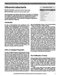
Introduction This tutorial provides instructions for meshing an internal flow in a straight pipe. A geometry and mesh like those shown to the right are created. Pointwise software is used to create a structured grid that has fine resolution near the wall and coarser resolution elsewhere. A pressure drop is calculated across the inlet and outlet of the pipe. OpenFOAM software is used as the CFD solver.

Straight Pipe Choose solver 1. This tutorial assumes that Pointwise is running. If it is not running, open it before proceeding to the next step. 2. CAE-Select Solver…-OpenFOAM It is wise to choose the desired CFD solver before creating any grids. Setting the solver first reduces the possibility of problems later when exporting the mesh. 3. OK. The current solver is displayed in the lower left corner of the Pointwise window. 4. File-Save. 5. After selecting an appropriate folder in which to save the project, enter “Straight_Pipe” for the File name. 6. Save.

Create geometry in Pointwise 1. Because of symmetry, it is not necessary to model the entire pipe. Only one-quarter of the pipe will be analyzed. Splitting the geometry in this way reduces the analysis time by approximately 75%. 2. View-Toolbars, and verify that all toolbars are activated (a checkmark by each title). 3. Defaults tab under Panels. Make sure the box to the left of Connector is checked. 4. Enter “21” as the default dimension. The default dimension is the number of nodes assigned to each connector created after setting the default. 5.

2 Point Curves from the Create toolbar. Hover the cursor over any toolbar button to display its name. Alternatively, Create-2 Point Curves... 6. Under Point Placement, type “0 0.02625 0” as the XYZ coordinates for the first endpoint. . Use the following format for entering Point Placement data: “x-coordinate” “ycoordinate” “z-coordinate”. Delete Last Point if a wrong coordinate is entered. 7. Type “0 0 0” as the XYZ coordinates for the second endpoint. . 8. again to place another point at “0 0 0”. 9. Type “0.02625 0 0”. . 10. Type “0 0.02625 0.68247”. . 11. Type “0 0 0.68247”. .

Tutorial – Laminar Flow through a Straight Pipe, Page 2

12. again to place another point at “0 0 0.68247”. 13. Type “0.02625 0 0.68247”. . 14. OK. 15. List tab. LMB the “+” next to Connectors in the List panel. The expanded list shows the type of connector and the number of points assigned to each one. You should have 4 connectors. 16. Rotate the axis to an isometric view by holding down and the RMB while moving the cursor to the left. 17. View-Zoom-Zoom to Fit. Alternatively, press on the keyboard. 2 Point Curves. 18. 19. LMB Point1, then LMB Point2 to create a long connector. 20. LMB Point3, then LMB Point4 to create a second long connector. 21. LMB Point5, then LMB Point6 to create a third long connector 22. OK. 23.

Curve from the Create toolbar. Alternatively, Create-Draw Curves-Curve. 24. Circle. Select 2 Points & Center under Circle Segment Options. 25. LMB Point1, then LMB Point5. LMB Point3 to place the center of the circle. Apply. 26. LMB Point2, then LMB Point6. LMB Point4 to place the center of the circle. Apply. 27. OK. 28. List tab. You should now have 9 connectors. A “connector” is the Pointwise terminology for a mesh construction line.

Modify axial dimensions 1. Simultaneously select the three longest connectors (“con-5”, “con-6”, and “con-7”). Hold while LMB to make multiple selections. Selections can be made in the graphics window or from the List panel. 2. Grid-Dimension… 3. Type “100” as Number of Points. Dimension-OK. These points will space the mesh cells in the axial direction. Sometimes it is helpful to make the spacing points visible. To do this, select a connector(s) and choose “Points On” from the drop down menu beside “ Points Off” in the Attributes toolbar.

Create surface mesh on the pipe wall 1. Simultaneously select the closed loop of four connectors that form the perimeter of the curved pipe wall. These connectors form the framework for a mesh that will cover the curved surface. Hold while LMB to make multiple selections. Try selecting the connectors from the list under Connectors in the side panel. Select “con-5”, “con-7”, “con-8”, and “con-9”. 2. Structured in the Mesh toolbar. Alternatively, Grid-Set Type-Structured.

Tutorial – Laminar Flow through a Straight Pipe, Page 3

3.

Assemble Domains in the Create toolbar. A structured mesh with 100 axial divisions and 20 circumferential divisions is created on the pipe wall.

Extrude surface mesh 1. LMB the “+” next to Domains in the List panel. A “domain” is a surface grid in Pointwise. 2. Select “dom-1”. 3. Create-Extrude-Normal… 4. Boundary Conditions tab in the side panel. 5. LMB the long edge with the largest ycoordinate. 6. In the side panel, change Type from “Splay” to “Constant X”. Set Boundary Condition. It may be necessary to rotate (+RMB) and zoom (scroll MMB) to select the connector. 7. LMB the long edge with the largest x-coordinate. 8. Change Type from “Splay” to “Constant Y”. Set Boundary Condition. 9. Simultaneously select (+LMB) the circular edges on each end of the pipe (total of 2). 10. Change Type from “Splay” to “Constant Z”. Set Boundary Condition. 11. Attributes tab in the side panel. 12. LMB the box next to Step Size. 13. Enter “0.0001” for Initial ∆s. 14. Change the Growth Rate to “1.2”. 15. LMB the box next to Orientation. 16. Flip only if the direction arrows in the graphics window are pointing away from the center of the pipe. 17. Run tab in the side panel. 18. Enter “10” for Steps. Run-OK.

Split connectors 1. Recall View -Z from the View toolbar. 2. View-Zoom-Zoom to Fit (or ). 3. You are now looking down the Z axis of the pipe. Notice the 10 layers of cells along the wall of the pipe. The surface mesh has been extruded into a block of cells. There should now be a (1) after Blocks in the List panel. A “block” refers to a volume grid in Pointwise. Unlike with some other mesh generators, the boundary layer mesh is considered as its own block. 4. LMB the vertical connector (con-3). 5. Edit-Split… 6. LMB Point7. 7. OK. 8. LMB the horizontal connector (con-4). 9. Edit-Split… 10. LMB Point8. 11. OK. 12.

Recall View +Z from the View toolbar.

Tutorial – Laminar Flow through a Straight Pipe, Page 4

13. View-Zoom-Zoom to fit (or ). 14. LMB the vertical connector (con-1). 15. Edit-Split… 16. LMB Point9. 17. OK. 18. LMB the horizontal connector (con-2). 19. Edit-Split… 20. LMB Point10. 21. OK. 22. Simultaneously select “con-3-split-1”, “con-4-split-2”, “con-1split-1”, and “con-2-split-2” from Connectors in the List panel. (Select all the connectors with “3” points.) 23. . 24. Select “con-14” from Connectors in the List panel. 25. Edit-Split... 26. Enter “50” for the Percent of Length. . 27. OK. The connector has been split into two separate connectors with 11 points on each.

Split the mesh block 1. 2. 3. 4. 5. 6.

LMB the “+” next to Blocks to expand the list. Select “blk-1”. Edit-Split… Select “J” as the Split Direction. LMB Point11. OK.

Insert connectors on end of pipe 1. Defaults tab. Make sure the box to the left of Connector is checked. 2. Enter “11” as the new default dimension. List tab. 3. 2 Point Curves. 4. Type “0.01 0 0” under Point Placement. . 5. Type “0.01 0.01 0”. . 6. Notice that a connector has been added in the graphical display. 7. again to place another point at “0.01 0.01 0”. 8. Type “0 0.01 0”. . 9. OK. 10. Rotate and zoom to get the perspective shown to the right. Zoom by scrolling the MMB. Rotate by holding and RMB while moving the cursor. to center and zoom to fit the geometry in the window. 11. 2 Point Curves. 12. Connect Point13 and Point11 by successively LMB on each point. 13. OK. 14. Follow the basic steps used in the section Split connectors to split the corner connectors at Point12 and Point14 as shown. Select line to be split. Edit-Split… Select point where split will occur. OK.

Tutorial – Laminar Flow through a Straight Pipe, Page 5

15. Simultaneously select the two newly split connectors that have 9 nodes. Select (“con-1-split-2-split-2” and “con-2-split-1-split-1) from under Connectors in the List side panel. 16. Grid-Dimension… 17. Enter “11” as the Number of Points. Dimension-OK. The “ Dimension” feature in the Grid toolbar can also be used to change the number of points on a connector. Select a connector(s). Enter a dimension in the toolbar Connectors opposite from each other must have the same number of points to create a structured grid.

. .

Create structured surface meshes on end of pipe 1. Simultaneously select the 9 connectors from the List panel as shown to the right. To make selecting an entire list of connectors easier, hold while LMB on the first and last entry of a list. 2. Grid-Merge… 3. Check the box next to Auto Merge (it may already be checked). 4. Set Tolerance to “.001”. . 5. OK. 6. Verify that Structured is the current grid type. toggle button is depressed in the Create Make sure the toolbar, or Grid-Set Type-Structured. 7. Assemble Domains.

Extrude domains along pipe length 1. 2. 3. 4. 5. 6. 7. 8.

Simultaneously select “dom-3”, “dom-5”, and “dom-6” from the List panel. Create-Extrude-Path… Done. List tab. Select “con-11”. “Con-11” is an axial connector that will guide the extrusion path. Path tab. Steps already should be set at “99”. Run-OK.

Define boundary conditions 1. 2. 3. 4. 5. 6.

7. 8.

CAE-Set Boundary Conditions… New. LMB “bc-2” and change the name to “inlet”. In the same row, “Unspecified” and choose “patch” from the drop down menu (you have to double click to get to the drop down menu). List tab from the side panel. Simultaneously select “dom-5-split-1”, “dom-5-split2”, “dom-13”, and “dom-18”. Alternately, you can select the four domains of the inlet plane manually with the mouse. Set BC tab from the side panel. LMB in the empty box next to the second row. A “4” should appear in the “#” column. This indicates that four domains have been defined as an inlet. Notice that of the 17 domains, 4 are now specified and 13 remain unspecified.

Tutorial – Laminar Flow through a Straight Pipe, Page 6

9. New. 10. LMB “bc-3” and change the name to “outlet”. 11. In the same row, “Unspecified” and choose “patch” from the drop down menu. 12. List tab. 13. Select the five domains on the opposite end of the pipe as the outlet (“dom-3-split-1”, “dom-3-split-2”, “dom3”, “dom-5”, and “dom-6”). 14. Set BC tab. 15. LMB in the empty box next to the third row. A “5” should appear in the “#” column, and 8 domains remain unspecified. 16. New. 17. LMB “bc-4” and change the name to “symmetry”. 18. In the same row, “Unspecified” and choose “symmetryPlane” from the drop down menu. 19. List tab. 20. Simultaneously select all the domains on both symmetry planes of the pipe (“dom-2”, “dom-4”, “dom-10”, “dom11”, “dom-12”, and “dom-17”). 21. Set BC tab. 22. LMB in the empty box next to the fourth row. A “6” should appear in the “#” column. 23. New. 24. LMB “bc-5” and change the name to “wall”. 25. In the same row, “Unspecified” and choose “wall” from the drop down menu. 26. List tab. 27. Select the two pipe wall domains (“dom-1-split-1” and “dom-1-split-2”). 28. Set BC tab. 29. LMB in the empty box next to the fifth row. A “2” should appear in the “#” column. 30. The boundary conditions should now be set as indicated to the right. Notice that all domains are now specified. 31. Close the BC tab.

Export CAE as OpenFOAM case 1. 2. 3. 4. 5. 6. 7. 8.

LMB the “+” next to Blocks in the side panel if it isn’t already expanded. Simultaneously select all the blocks (total of 4). File-Export-CAE… After selecting an appropriate location, create a new folder in which to export the project. Name the folder “polyMesh” . Choose or Save or OK, depending on your operating system. File-Save the Pointwise file. File-Exit Pointwise.

Create OpenFOAM “run” directory and copy tutorials OpenFOAM is a collection of open source C++ computer programs. Individual programs can be assembled into applications that can solve computational problems and manipulate data. In this tutorial a new mesh and initial conditions are applied to an existing application. 1. This tutorial assumes that a complete instillation of OpenFOAM and PyFoam exist on a local computer running on a Linux operating system.

Tutorial – Laminar Flow through a Straight Pipe, Page 7

PyFoam is a library of python language scripts that monitors runs in OpenFOAM. 2. Open a new terminal. The terminal can often be accessed from the graphical interface by Applications-AccessoriesTerminal. The exact location of the terminal may differ between computers. 3. In this tutorial, instructions are in black text and are followed by blue text strings that should be typed in the terminal. Press to execute the string after it is typed. The entry “[location string]” should be replaced with the desired directory location (the same location is used every time [location string] appears). An example of a location string is /home/username where “username” is replaced with the local user name. This tutorial can also be completed using a graphical interface. Navigate to desired directories by using the blue text as a guide. A “directory” is the same as a “folder”. 4. Create a directory named “run” within a new directory named “OpenFOAM”. 5. mkdir –p [location string]/OpenFOAM/run The command pwd gives the path to the current directory location. This tool can be used to determine the [location string] of a suitable location in which to create the new directories. 6. Copy a folder of OpenFOAM tutorials from the instillation directory to the newly created “run” directory. 7. cp –r $FOAM_TUTORIALS [location string]/OpenFOAM/run It is helpful to use these tutorials as templates for new cases. The tutorials are organized by their function. To quickly run a new case, modify an existing tutorial from a desired category.

Copy and rename “cavity” tutorial to the “run” directory 1. Navigate to the newly copied “tutorials” folder. Open the “incompressible” directory. Then open the “icoFoam” directory. The “incompressible” directory contains examples of standard solvers for incompressible fluids. The icoFOAM solver is a transient solver for laminar flow of incompressible, Newtonian fluids. 2. cd [location string]/OpenFOAM/run/tutorials/incompressible/icoFoam 3. Move and rename a copy of the “cavity” folder to the “run” directory. The following script copies the folder and renames it “straight_pipe”. 4. cp –r cavity [location string]/OpenFOAM/run/straight_pipe

Replace existing mesh data with files exported from Pointwise 1. Locate and open the new directory named “straight_pipe”. Then, open the “constant” folder. 2. cd [location string]/OpenFOAM/run/straight_pipe/constant 3. Delete the existing directory called “polyMesh”. The directory with files exported from Pointwise will replace this folder. 4. rm –r polyMesh 5. Navigate to the location of the “polyMesh” folder that was exported from Pointwise. 6. Move new “polyMesh” directory to the “constant” folder. 7. mv polyMesh [location string]/OpenFOAM/run/straight_pipe/constant 8. The files should now be organized as mapped in the image below. The red names are directories, and the black names are files.

Tutorial – Laminar Flow through a Straight Pipe, Page 8

Change initial conditions in the “p” and “U” files 1. Open the “polyMesh” folder. 2. cd [location string]/OpenFOAM/run/straight_pipe/constant/polyMesh 3. Open the “boundary” file in the background with a text editor. Executing a command the background allows a user to enter additional commands in the terminal without completing previous commands. 4. gedit boundary & Here, “gedit” is the text editor used to open the “boundary” file. Other text editors (such as vi) can be used if “gedit” isn’t available. Adding an ampersand (&) after any command causes it to execute in the background. 5. The “boundary” file lists all the boundary conditions that were assigned and named in Pointwise. The names of these boundary conditions (inlet, outlet, symmetry, and wall) must be entered in the initial pressure (p) and velocity (U) files. Keep the “boundary” file open so the boundary names are visible. 6. Locate and open the “0” directory. The “0” directory contains pressure and velocity files at the initial time (t=0). After the case is solved, additional directories that correspond to each time steps will be added in the “run” directory. 7. cd [location string]/OpenFOAM/run/straight_pipe/0 8. Open the initial pressure “p” file in the background. 9. gedit p & 10. In the open “p” file, change the boundary names and pressure conditions to match those seen in the “boundary” file. Make changes until the text between the dividing lines exactly matches that seen below.

Tutorial – Laminar Flow through a Straight Pipe, Page 9

The dimension is set by indicating the power of each base unit within the [ ] brackets. The base units are listed in the following order: [mass length time temperature quantity current luminous]. The initial value of the internal pressure field is uniform and equal to zero. The inlet and wall boundaries are set to type zeroGradient. This means that solved values at these boundaries must be constant for progressive elements in the direction normal to the boundary surface (the normal gradient equals 0). The actual values will be numerically calculated by the solver. The type symmetryPlane indicates that there is a plane of symmetry on the selected faces. Notice that the value for the outlet pressure is a scalar and is set equal to a fixed value of 0 (open to the atmosphere). 11. Save when all the changes have been made. 12. Close the “p” file. 13. Navigate to initial velocity “U” file, and then open it in the background using a text editor. 14. gedit U & 15. In the open text file change the boundary names and conditions until the text between the dividing lines matches that seen below. Values of the internal velocity field are uniform and each component of the initial vector is set to zero. Only the outlet velocity is set to type zeroGradient. This means that the outlet velocity must be constant for progressive elements in the direction normal to the outlet surface (the normal gradient equals 0). The actual values will be numerically calculated by the solver. The type symmetryPlane indicates that there is a plane of symmetry on the selected faces. Notice that the value for the inlet velocity is a vector and is set to flow at -.04 m/s along the negative z-axis, making the flow normal to the inlet face. The wall velocity vector is set to (0 0 0) to enforce the no-slip boundary conditions at a stationary wall. 16. Save when all the changes have been made. 17. Close the “U” file. 18. Close the “boundary” file.

Set kinematic viscosity (nu) 1. 2. 3. 4. 5.

Navigate to the “constant” directory. cd [location string]/OpenFOAM/run/straight_pipe/constant Open “transportProperties” with a text editor. gedit transportProperties Change the value of nu from “.01” to “1e-6” as indicated below. The kinematic viscosity of water at 20o C is approximately 1.0 x 10-6 m2/s.

Tutorial – Laminar Flow through a Straight Pipe, Page 10

The dimension is set by indicating the power of each base unit within the [ ] brackets. The base units are listed in the following order: [mass length time temperature quantity current luminous].

6. Save and then close the “transportProperties” file.

Change run-time settings IcoFOAM is a time dependent solver. A user can define a period over which the solver should iterate a solution. Multiple iterations are performed at each user time step. The solution to each time step is saved in a separate directory. This allows users to examine time dependent characteristics such as flow development. 1. Navigate to the “system” directory. 2. cd [location string]/OpenFOAM/run/straight_pipe/system 3. Open “controlDict” with a text editor. 4. gedit controlDict 5. The settings here are sufficient for this case. Notice that the start time, end time, and time steps can be easily modified from this file. The iterations will march at a time step (deltaT) of 0.005 seconds until .5 second is reached (a total of 100 time steps). However, only 5 time steps will be written to file because the writeInterval is set to 20. Only every 20th time step will be recorded and files will be generated for time steps 0, 0.1, 0.2, 0.3, 0.4, and 0.5. 6. Close the “controlDict” file.

Run icoFOAM solver 1. 2. 3. 4.

5. 6. 7. 8.

Navigate to the “straight_pipe” directory. cd [location string]/OpenFOAM/run/straight_pipe Run the solver in the background and create a log file. icoFoam > log & A “log” file is created within the case directory as the solver iterates a solution. This file documents the progress of the solver. Monitor real-time plots of residuals as the simpleFoam iterates a solution. pyFoamPlotWatcher.py log If PyFoam is not installed, skip this step. Wait until the solver is finished iterating a solution before proceeding to the next step. This takes some time, so be patient. After the solver is finished, close the residual plots and +C to break out of the monitoring.

Create vector component files 1. Velocity vectors are stored in “U” files for each time step. These vectors will be split into their scalar x, y, and z comments and stored in Ux, Uy, and Uv files in each time step directory. 2. foamCalc components U The magnitude of each vector can also be calculated and recorded in each time-step directory be executing the following command: foamCalc mag U

Tutorial – Laminar Flow through a Straight Pipe, Page 11

Calculate the pressure drop 1. The average inlet and outlet pressures will be calculated. The difference between these pressures is the pressure drop in the pipe. 2. Calculate the average pressure at the inlet for each time-step and store the results in a file named “inletAvP”. 3. patchAverage p inlet > inletAvP 4. Calculate the average pressure at the outlet for each time-step and store the results in a file named “outletAvP”. 5. patchAverage p outlet > outletAvP 6. View the average inlet pressures in the terminal window. 7. cat inletAvP 8. OpenFOAM normalizes pressure values by dividing the true pressure by the density of the working fluid. This normalization results in a number with units of m2/s2. To calculate the true gage pressure, multiply the average pressure at the last time-step by the density of the working fluid. Use 998.2 kg/m2 as the density of the working fluid for this case. The density of the working fluid was indirectly specified as 998.2 kg/m3 (density of water at 20oC) when the kinematic viscosity was assigned. 9. View the average outlet pressures. 10. cat outletAvP 11. The outlet gage pressure should be zero because the outlet boundary condition was specified as zero gage pressure.

Launch ParaView 1. 2. 3. 4.

If not already there, navigate to the “straight_pipe” directory. cd [location string]/OpenFOAM/run/straight_pipe Launch ParaView. paraFoam

View results in ParaView 1. In ParaView, make sure that the Properties tab is selected in the Object Inspector panel. 2. LMB “Show Patch Names”. 3. LMB the box next to mesh parts “inlet-patch” and “outlet-patch”. 4. LMB “Volume Fields” to select all the variable. 5. Apply. 6. LMB on the Display tab in the Object Inspector panel. 7. Scroll down to the Style section. Change Representation from “Outline” to “Surface” by using the dropdown menu. 8. Rotate and zoom in the graphical display to better see the solid model. Rotate by holding LMB while moving the cursor. Zoom by scrolling the MMB. 9. View-Toolbars. 10. Activate all the toolbars by LMB to place a before any unmarked titles.

View pressure distribution

Tutorial – Laminar Flow through a Straight Pipe, Page 12

1. Select the Display tab. 2. Scroll down to the Color section. ” from the dropdown 3. Change Color by to “ menu. Nothing has changed in the graphical display because the current time-step is zero. 4.

Last Frame in the VCR Controls toolbar to move to the last time step. Alternatively, enter a specific time-step in the Current Time Controls toolbar. Next Frame to move through individual time-steps.

5.

Rescale to Data Range in the Active Variable Controls toolbar.

6.

Toggle Color Legend Visibility. Alternatively, View- Show Color Legend. 7. The maximum pressure should be located at the inlet and have a value similar to the average normalized inlet pressure calculated in OpenFOAM as shown to the right.

View velocity field 1. Select the Properties tab. 2. Unselect “Show Patch Names”. 3. Unselect “internalMesh” and “inlet-patch”. 4. Apply. 5. Filters-Alphabetical-Cell Centers. 6.

Apply.

7. With “

CellCenters1” still selected in the Pipeline Browser,

Alternatively, Filters-Alphabetical8. Verify that the Glyph Type is set to “Arrow”. 9. Scroll down to the Orient section. 10. Change Scale Mode from “vector” to “off”. 11. LMB the box next to “Edit”.

Glyph.

Glyph.

12.

Apply.

13.

Toggle Color Legend Visibility and set the variable to in the Active Variable Controls toolbar.

14. Set view direction to +Z. 11. Rotate and zoom in the graphical display to better see the velocity vector field. It should look similar to the vector field to the right. Rotate by holding LMB while moving the cursor. Zoom by scrolling the MMB.

Tutorial – Laminar Flow through a Straight Pipe, Page 13

Save the ParaView case 1. File-Save State. 2. After selecting the case directory as the location in which to save the ParaView state, enter “Velocity_field” as the File name. 3. OK. 4. File-Exit.