POL 681 Problem Set 1: Regression and Correlation Review. ANSWER KEY. 1.
The correlation coefficient is given by: r = Σ(xi − x)(yi − y). √. Σ(xi − x)2Σ(yi − y)2.
POL 681 Problem Set 1: Regression and Correlation Review ANSWER KEY 1. The correlation coefficient is given by: r=�
Σ(xi − x)(yi − y) Σ(xi − x)2 Σ(yi − y)2
.
For these data, the numerator is equal to -15862.67 and the denominator is equal to 21155.82. The correlation is thus -.75. 2. Substantively, we see that money and votes are negatively correlated. This leads to the conclusion that as campaign spending on the part of the incumbent increases, the number of votes he/she receives decreases. There is an inverse relationship. 3. The graph of votes versus money looks like Figure 1. The negative relationship described by the correlation coefficient is clearly seen (although there are obviously few data points here).
70
votes
65
60
55
50 0
1000 money
500
1500
2000
Scatterplot of votes and money spent among Arizona House incumbents in 1998 election.
4. The estimated regression slope in the bivariate case is given by: Σ(xi − x)(yi − y) . Σ(xi − x)2 . The numerator is equal to -15862.67 and the denominator is equal to 1725844.8. The slope coefficient is thus -.00919. As a side note, if you were to compute the variance of money, it would be 345,169. This is 1
different from the denominator here. Recall that the variance is the sum of the squared mean deviations divided by n−1. In order to get the denominator, multiply the variance by n−1 which is 345169×5 = 1725845. For the intercept, note that it is given by ¯. βˆ0 = y¯ − βˆ1 x For this problem, the mean of y is 61.67 and the mean of x is 683.17. Thus, the intercept is 67.95 (after substituting in βˆ1 = −.00919). The regression model is: ˆ i = 67.95 − .00919(M oneyi ). V otes
5. The negative slope coefficient tells me that money and expected votes are negatively related. Specifically, I see that for a $100000 increase in spending, the expected number of votes drops by about .92 percent. Thus, for every $110000 increase in spending, the expected number of votes drop by about 1 percent. In short, votes and money are inversely related. The intercept has no real interpretation. Technically, it says that the expected number of votes is 67.95 percent when an incumbent spends no money. But since x = 0 is not observed in the data, the interpretation of this coefficient in this way does not make a lot of substantive sense. 6. The graph of the data and the predicted regression line is shown in Figure 2.
votes
Fitted values
70
65
60
55
50 0
1000 money
500
1500
2000
Scatterplot of votes and money spent among Arizona House incumbents in 1998 election along with predicted values from regression model.
2
7. The variance components are given by: SSE = Σ(yi − yˆi )2 , and
SSR = Σ(yˆi − y)2 .
The SSR is equal to 145.80 and the SSE is equal to 113.54. 8. The r2 is a ratio of “explained variance” (given by the SSR) to the total variance (given by SSR+SSE=SSTO). Thus, the r2 = SSR/SSR+SSE. For these data, the r2 is about .56. 9. There is a lot of unexplained variance in y; however, the majority of the variation in y is accounted for by knowledge of x. A superior model might include other information, for example, data on the challenger. However, as a simple regression model, predictions of votes based on money spent are better than simply guessing the mean number of votes. That is, the model improves our ability to predict votes above and beyond relying on the mean of votes. 10. The inverse finding is expected because the more money an incumbent spends is probably in relation to the amount of money a challenger is spending. Strong challengers can spend more money (because they raise more money); thus, incumbents are forced to spend more money in response. As a result, their expected number of votes decrease when facing a strong challenger which produces the negative relationship we find here. Obviously, this is speculation. To actually test this, we would like to have data on challengers.
3