Polar permutation graphs are polynomial-time recognisable∗ Tınaz Ekim†
Pinar Heggernes‡
Daniel Meister‡
Abstract Polar graphs generalise bipartite graphs, cobipartite graphs, and split graphs, and they constitute a special type of matrix partitions. A graph is polar if its vertex set can be partitioned into two, such that one part induces a complete multipartite graph and the other part induces a disjoint union of complete graphs. Deciding whether a given arbitrary graph is polar, is an NP-complete problem. Here, we show that for permutation graphs this problem can be solved in polynomial time. The result is surprising, as related problems like achromatic number and cochromatic number are NP-complete on permutation graphs. We give a polynomial-time algorithm for recognising graphs that are both permutation and polar. Prior to our result, polarity has been resolved only for chordal graphs and cographs.
1
Introduction
Many graph problems can be formulated as finding a partition of the vertices such that various parts satisfy certain properties internally, and at the same time certain other properties are satisfied regarding the interaction between these parts. Examples of such problems are the broad variety of colouring and homomorphism problems, and the matrix partition problem; the latter was posed by Feder et al. [15]. The matrix partition problem asks for a partition of the vertex set of a graph into subsets A1 , . . . , Ak such that each subset is either a clique or an independent set, and pairs of subsets are completely adjacent or completely non-adjacent, depending on a given pattern. If the pattern says that we partition into only cliques and independent sets, and two partition sets Ai , Aj should be completely adjacent if Ai , Aj are independent sets, completely non-adjacent if Ai , Aj are cliques, and there is no restriction for the two other cases, then we get exactly the polar graphs. Polar graphs were defined in 1985 by Tyshkevich and Chernyak [26]. A graph is polar if its vertex set can be partitioned into A and B such that A induces a complete multipartite graph and B induces a cluster graph, i.e., a disjoint union of complete graphs. Such a partition is called polar. Since complements of cluster graphs are exactly complete multipartite graphs (and vice versa), the class of polar graphs is closed under taking complements. Furthermore, it contains the well-known classes of split graphs, bipartite graphs, and cobipartite graphs. If A is simply an independent set, then the graph (and the partition) is called monopolar. In addition to fitting into the matrix partition problem [15] described above, polar partitions can be seen as generalised colourings [5]. ∗
This work was supported by the Research Council of Norway, and the first author was supported by the B. U. Research Fund, grant 09A302P. A preliminary version of the paper was presented at IWOCA 2009 [10]. † Industrial Engineering Department, Bo˘ gazi¸ci University, Istanbul, Turkey. Email:
[email protected] ‡ Department of Informatics, University of Bergen, Norway. Emails:
[email protected],
[email protected]
1
B
⧹
A
indep. set clique
indep. set
clique
cluster gr.
compl. multip.
P
P
P
?
P
?
P
?
P
cluster gr. compl. multip.
?
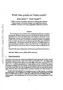
Figure 1: The table shows known and new computational complexity results for (A, B)-partition problems on permutation graphs, when A or B (symmetrically) is an independent set, is a clique, induces a cluster graph, or induces a complete multipartite graph. The boldface entries are the results of this paper. Empty cells are due to the symmetry of the table. The recognition problems for polar and monopolar graphs are NP-complete [6, 14]. Notice, however, that “admitting a polar partition” can be expressed in monadic second-order logic without using edge-set quantification, and hence, polar graphs of bounded treewidth or bounded clique-width can be recognised in polynomial time, by the results of [1, 8] and [9]. Consequently, it is of interest to find out where the boundary goes between subclasses of polar graphs that are recognisable in polynomial time and those whose recognition is intractable. When it comes to graph classes of unbounded treewidth and clique-width whose intersection with polar graphs can be recognised in polynomial time, so far we know only of chordal graphs [11, 17]. In this paper, we give polynomial-time algorithms for the two problems of deciding whether a given permutation graph is polar or monopolar. Permutation graphs are a well-studied graph class with a large number of theoretical applications [4, 18], and they can be recognised in linear time [24]. Permutation graphs have unbounded treewidth and clique-width [19]. Although many NP-complete problems become tractable on permutation graphs, well-known colouring problems, like cochromatic number [16, 28] and achromatic number [2], remain NP-complete on this graph class. The class of monopolar graphs generalises bipartite graphs and split graphs, and thus the class of monopolar permutation graphs is a generalisation of the class of bipartite permutation graphs. Since permutation graphs are closed under taking complements, our recognition algorithm for monopolar permutation graphs can also be used to recognise polar permutation graphs whose B-set induces a complete graph. Thus, combined with the well-known recognition results for bipartite graphs, split graphs and cobipartite graphs, our results show that a range of partition problems, in the sense of the introductory matrix partition problem, are polynomial-time solvable on permutation graphs. We summarise these known and new results in Figure 1. We show separately that monopolar permutation graph recognition and polar permutation graph recognition is polynomial-time solvable. The algorithm for the monopolar case partitions the input graph into small split graphs that satisfy certain conditions. The running time of this algorithm is O(nm), which is a significant improvement from its preliminary version [10]. For the case of polar permutation graphs, the main idea is to delete a suitable set of vertices to reduce the problem to a generalised monopolar recognition problem. As a result, we obtain an O(nm2 )time algorithm for recognising polar permutation graphs, which improves the running time of the preliminary version in [10]. We consider the monopolar permutation graph recognition problem in Section 3, and the polar permutation graph recognition problem in Section 4. 2
Other results on polynomial-time recognisable subclasses of polar graphs include [25] which studies polar partitions where the size of each independent set and clique is bounded, [11, 17] which give forbidden subgraph characterisations and a recognition algorithm for polar chordal graphs, and [13] which gives similar results for polar cographs. In addition, [22] and [12] give respectively a forbidden subgraph characterisation and a polynomial-time recognition algorithm for bipartite graphs whose line graphs are polar. Finally, [7] gives a polynomial-time recognition algorithm for monopolar claw-free graphs. Another research direction is to study which NPcomplete problems become tractable on polar graphs. For example, [23] gives polynomial-time algorithms for finding a minimum maximal independent set in some subclasses of polar graphs. This problem remains NP-hard in polar graphs admitting a polar partition where the size of every independent set is at most one and the size of every clique is at most two.
2
Definitions and notation, polar partitions, and permutation graphs
Our input graphs are simple and undirected. Only in Section 3, we use directed graphs (digraphs) as auxiliary tools. Let G be a simple and undirected graph. We denote its vertex set by V (G) and its edge set by E(G). An edge between vertices u and v is denoted by uv. If uv is an edge of G then u and v are adjacent in G. For a vertex x of G, the neighbourhood of x, denoted as NG (x), is the set of vertices that are adjacent to x, and NG [x] = NG (x) ∪ {x}. The degree of a vertex x is dG (x) = |NG (x)|. Let X be a set of vertices of G. The subgraph of G induced by X is denoted as G[X] and defined as the graph on vertex set X and edge set the set of edges of G that join only vertices in X. By G \ X, we denote the graph G[V (G) \ X]. A graph is called complete if every pair of vertices is adjacent. A set X ⊆ V (G) is called a clique if G[X] is complete, and it is called an independent set if G[X] has no edges. A graph is connected if there is a path between every pair of vertices; otherwise, the graph is called disconnected. The connected components of a graph are the maximal connected (induced) subgraphs. The disjoint union of two graphs G and H is the graph on vertex set V (G) ∪ V (H) and edge set E(G) ∪ E(H); the disjoint union of more than two graphs is defined analogously. The complement of G, denoted as G, is the graph on vertex set V (G) and edge set {uv ̸∈ E(G) | u, v ∈ V (G) and u ̸= v}. A complete multipartite graph is the complement of the disjoint union of complete graphs. Equivalently, the vertex set of a complete multipartite graph admits a unique partition into maximal independent sets. For a given graph G, a partition (A, B) of V (G), where A or B can also be empty, is called polar if G[A] is a complete multipartite graph and G[B] is a disjoint union of complete graphs, i.e., a cluster graph. Equivalently, (A, B) is a polar partition for G if both G[A] and G[B] are cluster graphs. Note that (A, B) is a polar partition for G if and only if (B, A) is a polar partition for G. A polar partition (A, B) for G is called monopolar if A is an independent set in G. We say that a polar partition (A, B) for G is B-maximal if there is no polar partition (A′ , B ′ ) for G with B ⊂ B ′ . Note that, for a polar partition (A, B), if there is a vertex u in A without a neighbour in B then (A\{u}, B∪{u}) is also a polar partition for G. Hence the following result is immediate. Lemma 2.1 Let (A, B) be a B-maximal polar partition for a graph G. Every vertex in A has a neighbour in B. 3
A graph G is called split graph if V (G) admits a partition (A, B) such that A is an independent set of G and B is a clique of G. Such a partition is called split partition. It holds that split graphs are special monopolar graphs and split partitions are special monopolar partitions. Let n ≥ 1 and π be a permutation over {1, . . . , n}, i.e., a bijection between {1, . . . , n} and {1, . . . , n}. We will denote π equivalently as a permutation sequence (π(1), . . . , π(n)). The position of an integer x in π is π −1 (x). By π −1 (X) for X ⊆ {1, . . . , n}, we mean {π −1 (x) | x ∈ X}. The inversion graph of π has vertex set {1, . . . , n} and two vertices u, v are adjacent if and only if (u − v)(π −1 (u) − π −1 (v)) < 0. A graph is a permutation graph if it is isomorphic to the inversion graph of a permutation sequence [4, 18]. Permutation graphs can be recognised in linear time [24]. Permutation graphs also have a geometric intersection model: for two horizontal lines, mark n points on each line, assign to each point on the upper line a point on the lower line, and connect the two points by a line segment. The corresponding graph has a vertex for every line segment and two vertices are adjacent if the corresponding line segments cross. This representation is called a permutation diagram. A graph is a permutation graph if and only if it has a permutation diagram. Given a permutation graph, a permutation diagram for it can be computed in linear time [24]. It is important to note that every induced subgraph of a permutation graph is a permutation graph. For our purposes, we assume that a permutation graph is given as a permutation sequence and equal to the defined inversion graph. Every permutation graph with permutation sequence π has a permutation diagram D in which the endpoints of the line segments on the lower line appear in the same order as they appear in π. For such pairs (π, D), we say that D corresponds to π. For convenience reasons, sometimes we will not distinguish between vertices of the graph and line segments in the permutation diagram; however, the meaning will always be clear. Line segments, and thus vertices, have an upper and a lower endpoint.
3
Recognising monopolar permutation graphs
A polar graph G is monopolar if it has a polar partition (A, B) such that A is an independent set of G. Monopolar graphs are thus a generalisation of bipartite graphs and split graphs. We show in this section that monopolarity is polynomial-time decidable for permutation graphs. Our algorithm has running time O(nm) and is even able to output a monopolar partition, if such exists. Since connected bipartite graphs admit unique partitions and since partitions for split graphs are very restricted, an interesting question is whether connected monopolar graphs have a similar property regarding monopolar partitions. A simple example shows that this is not the case: a simple path is a monopolar graph, since it is bipartite, but it has exponentially many monopolar partitions. The algorithm that we present in this section is able to answer an even more general question: given a connected permutation graph G and a set F ⊆ V (G), does G have a monopolar partition (A, B) such that A ⊆ F . By choosing F = V (G), we get exactly the monopolar permutation graph recognition problem. We partition this section into two parts. In the first part, we present the main algorithmic idea. It is based on a partition of the graph into small split graphs. In the second part, we consider implementation aspects. As important auxiliary results, we will closely consider split partitions.
4
Figure 2: The figure shows a trapezoid (in grey) and some of the vertices in the intersection of the trapezoid, as it may appear in a permutation diagram. The vertices form an independent set.
3.1
Algorithm and correctness
Let G be a permutation graph with permutation sequence π and corresponding permutation diagram D. A trapezoid in D is a pair (I1 , I2 ) of intervals of integers with I1 = {i1 , . . . , i′1 } and I2 = {i2 , . . . , i′2 } for 1 ≤ i1 ≤ i′1 ≤ |V (G)| and 1 ≤ i2 ≤ i′2 ≤ |V (G)|. Trapezoids are the main substructures in permutation diagrams that we consider in this paper. We define four sets of vertices for trapezoids. Let T = (I1 , I2 ) be a trapezoid in D with I1 = {i1 , . . . , i′1 } and I2 = {i2 , . . . , i′2 }. We define the left side, the right side, the containment and the intersection of T: – left side: – right side:
L(T) =def {x ∈ V (G) | x < i1 and π −1 (x) < i2 } R(T) =def {x ∈ V (G) | i′1 < x and i′2 < π −1 (x)}
– containment: con(T) =def {x ∈ V (G) | i1 ≤ x ≤ i′1 and i2 ≤ π −1 (x) ≤ i′2 } – intersection: int(T) =def V (G) \ (L(T) ∪ R(T)) . Note that con(T) ⊆ int(T). For X ⊆ V (G), the X-trapezoid in D is the trapezoid U = (J1 , J2 ) with J1 = {min X, . . . , max X} and J2 = {min π −1 (X), . . . , max π −1 (X)}. Furthermore, X ⊆ con(U). Informally, the X-trapezoid is the smallest trapezoid that contains X. Every trapezoid is not necessarily an X-trapezoid for some set X. A schematic example of a trapezoid in a permutation diagram, with some vertices in its containment and intersection, is shown in Figure 2. It follows from the properties of cliques in permutation diagrams that min π −1 (X) = π −1 (max X) and max π −1 (X) = π −1 (min X) when X is a clique. Our solution of the problem in this section is based on the following idea: Let (A, B) be a monopolar partition. Then every clique in G[B] can be connected to a trapezoid, and every vertex in A intersects with some trapezoid. For X ⊆ V (G) with 1 ≤ |X| ≤ 2, we call the X-trapezoid T good (with respect to F ) if G[int(T)] has a split partition (C, D) so that int(T) \ con(T) ⊆ C ⊆ F and X ⊆ D ⊆ con(T). We call this split partition (C, D) good for T (with respect to F ). For our algorithm, we construct an auxiliary digraph whose vertices correspond to the good trapezoids, and our problem is solved by deciding the existence of a path. In a digraph edges are ordered pairs, and they are called arcs. An arc from vertex u to vertex v is denoted by (u, v). A path in a digraph follows the directions of the arcs; hence there is a path (x1 , x2 , . . . , xs ) if there are arcs (x1 , x2 ), (x2 , x3 ), . . . , (xs−1 , xs ). Such a path from x1 to xs is called an x1 , xs -path. Let G be a permutation graph with permutation sequence π and corresponding permutation diagram D, and let F ⊆ V (G). By aux(D, F ), we denote the auxiliary digraph with the following vertices and arcs: 5
– aux(D, F ) has a vertex for every good X-trapezoid where X ⊆ V (G) and 1 ≤ |X| ≤ 2; denote by Tx the trapezoid that corresponds to vertex x of aux(D, F ); – for two vertices u and v of aux(D, F ), (u, v) is an arc in aux(D, F ) if con(Tv ) ⊆ R(Tu ) and R(Tu ) ∩ L(Tv ) = ∅ and (int(Tu ) \ con(Tu )) ∪ (int(Tv ) \ con(Tv )) is an independent set of G. To complete the definition of aux(D, F ), there are two more vertices, 0 and 1, and there is an arc (0, x) for every vertex x in aux(D, F ) with L(Tx ) = ∅, and there is an arc (x, 1) for every vertex x in aux(D, F ) with R(Tx ) = ∅. Lemma 3.1 Let G be a connected permutation graph with permutation sequence π and corresponding permutation diagram D. Let F ⊆ V (G). The auxiliary digraph aux(D, F ) has a 0, 1-path if and only if G has a monopolar partition (A, B) with A ⊆ F . Proof. Let P = (x0 , . . . , xs ) be a 0, 1-path in aux(D, F ). Note that s ≥ 2, since (0, 1) is not an arc of aux(D, F ) due to the definition of aux(D, F ). Let T1 , . . . , Ts−1 be the trapezoids corresponding to x1 , . . . , xs−1 , respectively. For 1 ≤ i ≤ s − 1, let (Ci , Di ) be a good split partition for Ti . We show that (C1 ∪ · · · ∪ Cs−1 , D1 ∪ · · · ∪ Ds−1 ) is a monopolar partition for G. First, observe that (C1 ∪ · · · ∪ Cs−1 ) ∩ (D1 ∪ · · · ∪ Ds−1 ) = ∅. Otherwise, there are x ∈ V (G) and 1 ≤ i, j ≤ s − 1 with i ̸= j such that x ∈ Ci ∩ Dj . By definition of good split partition, this particularly means that x ∈ con(Tj ). Since con(Ti ) ∩ con(Tj ) = ∅ due to the definition of the arcs of aux(D, F ), it holds that x ∈ int(Ti ) \ con(Ti ). Then, however, con(Tj ) ∩ int(Ti ) ̸= ∅, which is a contradiction to the properties of permutation diagrams and the definition of the arcs of aux(D, F ). Second, we show that (C1 ∪ · · · ∪ Cs−1 ) ∪ (D1 ∪ · · · ∪ Ds−1 ) = V (G). Suppose there is x ∈ V (G) such that there is no 1 ≤ i ≤ s − 1 with x ∈ int(Ti ). Since L(T1 ) = ∅ and R(Ts−1 ) = ∅, there is 1 ≤ i < s − 1 such that x ∈ R(Ti ) ∩ L(Ti+1 ). This, however, contradicts the definition of the arcs of aux(D, F ). We conclude that (C1 ∪ · · · ∪ Cs−1 , D1 ∪ · · · ∪ Ds−1 ) defines a partition for G. Since Di ⊆ con(Ti ) for every 1 ≤ i ≤ s − 1 and con(Ti ) ∩ con(Tj ) = ∅ for every 1 ≤ i < j ≤ s − 1, G[D1 ∪ · · · ∪ Ds−1 ] is the disjoint union of complete graphs. It remains to show that C1 ∪ · · · ∪ Cs−1 is an independent set of G. Suppose the contrary, i.e., there are u, v ∈ V (G) and 1 ≤ i ≤ j ≤ s − 1 with u ∈ Ci and v ∈ Cj and uv ∈ E(G). Note that i ̸= j since (Ci , Di ) is a split partition for G[int(Ti )] and therefore Ci is an independent set of G. If j − i ≥ 2 then u ∈ Ci+1 or v ∈ Cj−1 , so that we can assume without loss of generality that j − i = 1. Since u ̸∈ con(Ti ) and v ̸∈ con(Tj ), u and v are contained in (int(Ti ) \ con(Ti )) ∪ (int(Tj ) \ con(Tj )), which is an independent set of G due to the definition of the arcs of aux(D, F ). We obtain our contradiction, and the defined partition of V (G) is a monopolar partition for G. And with the condition Ci ⊆ F for every 1 ≤ i ≤ s − 1, we conclude that (C1 ∪ · · · ∪ Cs−1 , D1 ∪ · · · ∪ Ds−1 ) is a monopolar partition for G of the desired form. For the converse, let (A, B) be a monopolar partition for G with A ⊆ F . Let D1 , . . . , Dr be the sets of vertices that induce the connected components of G[B]. Without loss of generality, we can assume that min D1 < · · · < min Dr . With the properties of permutation diagrams, it follows that min D1 ≤ max D1 < · · · < min Dr ≤ max Dr . By definition of monopolar partition, D1 , . . . , Dr are cliques of G. For every 1 ≤ i ≤ r, let Xi =def {min Di , max Di } and let Ti be the Xi -trapezoid in D. By the properties of permutation diagrams, Di ⊆ con(Ti ). And since G[B] is the disjoint union of cliques, it follows with our assumption that con(Ti+1 ) ⊆ R(Ti ) for every 1 ≤ i ≤ r − 1. First, we show that for every 1 ≤ i ≤ r, Ti is good with respect to F . It 6
holds that 1 ≤ |Xi | ≤ 2. Since B ∩ con(Ti ) = B ∩ int(Ti ) = Di , it holds that int(Ti ) \ Di ⊆ A. Hence, ((int(Ti ) \ Di , Di ) is a split partition for G[int(Ti )] that is good. It follows that there is a vertex of aux(D, F ) that corresponds to Ti . Let x1 , . . . , xr be the vertices of aux(D, F ) that correspond to respectively T1 , . . . , Tr . Second, we show that (xi , xi+1 ) is an arc of aux(D, F ) for every 1 ≤ i ≤ r − 1. We have already seen that con(Ti+1 ) ⊆ R(Ti ). Since int(Ti )\con(Ti ) ⊆ A and int(Ti+1 )\con(Ti+1 ) ⊆ A due to the definition of Xi and Xi+1 , it holds that (int(Ti ) \ con(Ti )) ∪ (int(Ti+1 ) \ con(Ti+1 )) is an independent set of G. Finally, suppose that there is x ∈ V (G) with x ∈ R(Ti ) ∩ L(Ti+1 ). This means that x ̸∈ B, so that x ∈ A. Furthermore, x is not adjacent to any vertex in B, thus, x is an isolated vertex. This yields a contradiction to G being connected. We conclude that (xi , xi+1 ) is an arc of aux(D, F ). Third, we show that (0, x1 ) and (1, xr ) are arcs of aux(D, F ). Similar to the previous arguments, if L(T1 ) ̸= ∅ or R(Tr ) ̸= ∅ then there is a vertex in A without a neighbour in B, so that G cannot be connected. We conclude that aux(D, F ) has a 0, 1-path. Note that a 0, 1-path in aux(D, F ) does not correspond to a specific monopolar partition for G but can represent many partitions. The main reason is that a good split partition for a trapezoid is not unique, thus a vertex can belong to a clique and to the independent set in different monopolar partitions.
3.2
Running time
The main computational task is to construct the auxiliary digraph. We partition this task into listing the vertices and listing the arcs. For listing the vertices, the algorithm mainly needs to decide for a given trapezoid whether it is good. This is decided by checking the existence of a split partition that respects constraints. We want to decide this question in O(n) time per trapezoid, which requires a careful analysis of the structure of possible split partitions. Let G be a graph with at least one edge. The split partition number of G is defined as the smallest number k such that there are vertices u, v of G where dG (u) = k and dG (v) ≤ k and uv ∈ E(G). If G has a vertex of degree smaller than k then the largest degree k ′ with k ′ < k is called the second split partition number of G. Note that k ′ does not always exist. A split partition (C, D) for G is clique-maximal if there is no split partition (C ′ , D′ ) for G with D ⊂ D′ . Lemma 3.2 Let G be a split graph with at least one edge. Let k and k ′ be respectively the split partition number and the second split partition number of G (if the latter exists). Let (C, D) be a clique-maximal split partition. Then, one of the following holds: – C = {x | dG (x) < k} and D = {x | dG (x) ≥ k} – if k ′ exists: NG (x) = NG (x′ ) and xx′ ̸∈ E(G) for all vertex pairs x, x′ of G with dG (x) = dG (x′ ) = k ′ , and D = NG [y] for some vertex y with dG (y) = k ′ . Proof. We first show that all vertices of G with degree more than k belong to D. Let u, v be a vertex pair of G to witness the split partition number, i.e., dG (u) = k and dG (v) ≤ k and uv ∈ E(G). Suppose that there is a vertex x of G with dG (x) > k and x ∈ C. Since all neighbours of x are in D, it follows that |D| > k and all vertices in D with a neighbour in C have degree larger than k. Since u and v are adjacent, at most one of the two vertices can be in C. However, if one of the two vertices is in C then the degrees of u and v imply |D| ≤ k, in contradiction to the above lower bound on |D|. Thus, u, v ∈ D. This also implies 7
|D| = k + 1 due to |D| ≤ dG (u) + 1. Since dG (x) ≥ k + 1 and NG (x) ⊆ D, it follows that x is a neighbour of u. This implies dG (u) > k, which is a contradiction. Hence, x ∈ D, and therefore, {x | dG (x) > k} ⊆ D. Next, we consider vertices of degree smaller than k. Assume that there is a vertex y with dG (y) < k and y ∈ D. Suppose that y has a neighbour z in C. Then, y has at most k − 2 neighbours in D, which implies |D| ≤ k − 1, and thus dG (z) ≤ k − 1. This, however, contradicts the definition of the split partition number of G. Hence, all neighbours of y are in D, and since D is a clique of G, NG [y] = D. Note that all vertices in C have degree at most dG (y), since none of these vertices is adjacent to y. Suppose there is another vertex y ′ in D without a neighbour in C. Then, dG (y) = dG (y ′ ) and yy ′ ∈ E(G), contradicting the definition of the split partition number. Thus, all vertices in D \ {y} have degree more than dG (y). If there is a vertex z of G with dG (z) = dG (y) then z ∈ C by the above argument, and NG (z) = NG (y) due to the size of D. This particularly means that all vertices of degree dG (y) form an independent set of G. Furthermore, dG (y) = k ′ . This shows that (C, D) is a split partition for G of the second type. As the complementary case, we assume that all vertices of degree smaller than k are contained in C. With the result of the first paragraph, we thus have {x | dG (x) < k} ⊆ C and {x | dG (x) > k} ⊆ D. We consider the vertices of degree exactly k. Let E =def {x | dG (x) = k}. If E ⊆ D then (C, D) is a split partition for G of the first type. Otherwise let E ̸⊆ D. We show that this leads to a contradiction. By E ̸⊆ D, there is a vertex y ∈ E \ D. And since some vertex in E is adjacent to a vertex of degree at most k due to the definition of k, C ∪ E is not an independent set of G, thus there is x ∈ E ∩ D. Similar to the previous paragraph, if x has no neighbour in C then |D| = k + 1. Because of y ∈ C, all vertices in D \ {x} have a neighbour in C and thus degree at least k + 1. In particular, no vertex in E is adjacent to a vertex of degree at most k, which is a contradiction to the definition of the split partition number. Thus, x has a neighbour in C. Then, |D| ≤ k, and |D| ≥ k due to dG (y) = k. This implies |D| = k and that x has y as the only neighbour in C, in particular, C contains only y as a vertex from E. It follows that (C \ {y}, D ∪ {y}) is a split partition for G with D ⊂ D ∪ {y}, contradicting the assumption about (C, D) as being a clique-maximal split partition for G. This completes the proof. The result of Lemma 3.2 implies an efficient algorithm for checking whether a trapezoid is good with respect to some set of vertices. Lemma 3.3 There is an O(n)-time algorithm that, given a permutation graph G with permutation sequence π and corresponding permutation diagram D and sets F, F ′ ⊆ V (G) and each vertex labelled with its degree in G and the split partition number k of G (if it exists), decides whether G has a split partition (A, B) where F ′ ⊆ A ⊆ F . Proof. Let G, F , F ′ and k be the input according to the lemma. If F ′ is not an independent set of G or if F ′ ̸⊆ F then the algorithm immediately rejects. So, let F ′ be an independent set and F ′ ⊆ F . We want to apply Lemma 3.2. Observe that if G has a split partition (A, B) with F ′ ⊆ A ⊆ F then G has a clique-maximal split partition (A′ , B ′ ) with A′ ⊆ F and |B ′ ∩ F ′ | ≤ 1. Hence, for deciding the question it mainly suffices to consider clique-maximal split partitions. If G is edgeless then a desired split partition for G exists if and only if |V (G) \ F | ≤ 1. If G is a complete graph then a desired split partition for G exists if and only if |F ′ | ≤ 1. Using the degrees of the vertices, the two cases can be recognised and decided in O(n) time. Henceforth, let G be neither edgeless nor complete. Let k ′ be the second split partition number of G (if it exists). We check the following conditions: 8
1) G is a split graph 2) G has a clique-maximal split partition (A, B) with A ⊆ F . If G is a split graph then G has a split partition thus a clique-maximal split partition, and thus, one of the following vertex partitions is a split partition for G: – ({x | dG (x) < k}, {x | dG (x) ≥ k}) – if k ′ exists: (V (G) \ NG [y], NG [y]) for some vertex y with dG (y) = k ′ . As vertex y in the second case, we choose y with y ̸∈ F ′ if possible. The correctness of this check follows from the result of Lemma 3.2. In a second step, we check whether one of the two partitions yields a desired split partition. If k ′ does not exist then we have to consider only the first partition. Otherwise, if k ′ exists, and if y ′ ∈ F ′ for all vertices y ′ with dG (y ′ ) = k ′ then the second partition does not yield a desired partition. We consider the first partition; denote it by (A1 , B1 ). Clearly, if A1 ̸⊆ F then (A1 , B1 ) does not yield a desired partition. If F ′ ⊆ A1 ⊆ F then (A1 , B1 ) is a desired partition. Finally, assume that B1 ∩ F ′ = {x}. If x has at least two neighbours in A1 then (A1 , B1 ) does not yield a desired partition. If x has no neighbour in A1 then (A1 ∪ {x}, B1 \ {x}) is a desired partition. So, let x have exactly one neighbour in A1 , say z. Since dG (x) ≥ k and all vertices in A1 have degree smaller than k, z is non-adjacent to some vertex in B1 , and thus exchanging x and z does not yield a split partition. We consider the second partition, denoted as (A2 , B2 ). This case can be rejected if y cannot be chosen with y ̸∈ F ′ . Similar to the previous case, if B2 ∩ F ′ = {x} then we can accept if and only if x has at most one neighbour in A2 and the neighbour is adjacent to all vertices in B2 . For the running time of the algorithm, we see that, using the degree every vertex is labelled with, the vertex partitions can be computed straightforward in O(n) time. Also membership in F and F ′ is a simple table look-up for each vertex. We check whether a given set of vertices forms an independent set or a clique of G. Let S ⊆ V (G). In O(n) time, the vertices in S can be ordered by increasing upper endpoint in D. This ordering arranges the vertices by increasing lower endpoints if and only if S forms an independent set, and the ordering arranges the vertices by decreasing endpoints if and only if S forms a clique (for an illustration of the independent set case, see also Figure 2). This follows from the properties of permutation diagrams. The two properties can be verified in O(n) time. Scanning the degree labels, k ′ can be computed in O(n) time from k. All other checks can be executed in O(n) time. This completes the algorithm. For constructing the auxiliary digraph, we split the task into two subtasks, one of which is listing the vertices. To decide whether a trapezoid represents a vertex we have to decide whether the trapezoid is good, and we can apply the result of Lemma 3.3 to solve this problem. To obtain a complete algorithm, it remains to compute the split partition number. This can easily be done in linear time for arbitrary graphs. But we want to be faster. A partial algorithmic solution is given in the next lemma. Lemma 3.4 There is an O(n) time algorithm that given a split graph G whose vertices are labelled with their degrees in G, computes the split partition number of G. Proof. If G is edgeless then all vertices have degree 0 and the split partition number of G is undefined. If G is complete and has at least two vertices then all vertices have degree |V (G)| − 1 and the split partition number of G is |V (G)| − 1. This check requires O(n) time. Henceforth, 9
assume that G is not edgeless and not complete. Using the degree sequence of G, a split partition (I, C) for G can be computed in O(n) time (see, for instance, [18] and [20]). We observe, similar to the proof of Lemma 3.2, that all vertices in I have degree at most |C|, and all vertices in C with at least one neighbour in I have degree at least |C|. Let x be a vertex in C of smallest degree. Thus, if all vertices in C have a neighbour in I then the split partition number of G is equal to dG (x). Now, assume that x has no neighbour in I. It holds that dG (x) = |C| − 1 and all vertices in I have degree at most |C| − 1. Then, the split partition number of G is equal to min dG (C \ {x}). Note that C \ {x} is not empty, since otherwise G would be edgeless. This algorithm takes O(n) time. For permutation graphs, the split partition number can be computed in O(n log n) time: order the vertices by increasing degree, which defines a vertex ordering σ, and determine the leftmost vertex with a neighbour to its left. To decide the existence of a left neighbour, we assign to every vertex the number of vertices to its left in σ that have smaller upper endpoint in the permutation diagram and the number of vertices to its left in σ that have smaller lower endpoint in the permutation diagram. The two numbers are different for a vertex if and only if it has a neighbour to its left in σ. We leave it as an open problem whether the split partition number of a permutation graph with degree-labelled vertices can be computed in O(n) time. Now, we are ready for giving the main result and completing the main algorithm of this section. Theorem 3.5 There is an O(nm)-time algorithm that given a connected permutation graph G and a set F ⊆ V (G), decides whether there is a monopolar partition (A, B) for G with A ⊆ F . Proof. The algorithm is as follows: on input G a connected permutation graph with permutation sequence π and corresponding permutation diagram D and F ⊆ V (G), construct the auxiliary digraph aux(D, F ) and check whether aux(D, F ) has a 0, 1-path; accept if a 0, 1-path exists, otherwise reject. Due to Lemma 3.1, the algorithm accepts if and only if a desired monopolar partition for G exists. It remains to consider the running time of the algorithm, which is determined by the two tasks: constructing aux(D, F ) and finding a 0, 1-path. We begin with the construction of aux(D, F ). We first list the vertices of aux(D, F ) and then we list the arcs. Let G have n vertices and m edges. In linear time, we can label every vertex of G with its degree in G. By definition, aux(D, F ) has at most n + m vertices. Let X ⊆ V (G) with |X| = 1 and let T be the X-trapezoid. Note that X = con(T). It can be tested in O(n) time whether int(T) \ X is an independent set of G, and thus, it can be checked in O(n) time whether T is good. Now, let X ⊆ V (G) with |X| = 2, and let T be the X-trapezoid. To determine whether T is good, we have to decide for the vertices in con(T) which ones belong to the independent set and which ones to the clique. We compute the subgraph of G that is induced by int(T) and assign to every vertex its degree in G[int(T)]. For the vertices in con(T), the degree in G[int(T)] is equal to the degree in G. It remains to determine the degrees of the vertices in int(T) \ con(T); these are the vertices with neighbours in G that are not contained in int(T). If int(T) \ con(T) is not an independent set in G, then T cannot be a good trapezoid due to the definition of good trapezoid. So, let int(T) \ con(T) be an independent set. By the properties of permutation diagrams, the upper endpoint ordering is equal to the lower endpoint ordering of these vertices; let this ordering be σ. Let x be a vertex in int(T) \ con(T). It holds that dG[int(T)] (x) = dG (x) − |L(T) ∩ NG (x)| − |R(T) ∩ NG (x)|. We show that |L(T) ∩ NG (x)| and |R(T) ∩ NG (x)| can be computed in amortised constant time per vertex. If x < min X then 10
the upper endpoint of x is to the left of T, and |L(T) ∩ NG (x)| is equal to |x − min X| − 1 minus the number of vertices in σ to the right of x and with upper endpoint to the left of T. If π −1 (x) < π −1 (max X) then the lower endpoint of x is to the left of T, and |L(T) ∩ NG (x)| is equal to |π −1 (x) − π −1 (max X)| − 1 minus the number of vertices in σ to the right of x and with lower endpoint to the left of T. If none of the two cases holds then |L(T) ∩ NG (x)| = 0. For |R(T) ∩ NG (x)|, analogue equivalences hold. Since these numbers can be computed in overall O(n) time for all vertices in int(T) \ con(T), we conclude that we can compute a permutation diagram for G[int(T)] and assign the degrees to the vertices in O(n) time. As described in the proof of Lemma 3.4, we can check in O(n) time whether G[int(T)] is a split graph. If no then T is not good. If yes then we compute the split partition number of G[int(T)] using the algorithm of Lemma 3.4 and then we check whether G[int(T)] has a split partition (C, D) with int(T) \ con(T) ⊆ C ⊆ F ∩ int(T) by applying the algorithm of Lemma 3.3. Hence, in O(n) time, we can decide whether T is a good trapezoid with respect to F . Summarising, the set of vertices of aux(D, F ) and the corresponding good trapezoids can be determined in time O(nm). Now, we determine the arcs of aux(D, F ). We first give an algorithm for deciding whether there is an arc between two given vertices. Let u and v be vertices of aux(D, F ) and let Tu and Tv be the corresponding good Xu - and Xv -trapezoids. We decide whether (u, v) is an arc of aux(D, F ). According to the definition, we have to check three conditions. The condition con(Tv ) ⊆ R(Tu ) can be checked in constant time by verifying that max Xu < min Xv and π −1 (min Xu ) < π −1 (max Xv ). For the second condition, we check whether there is a vertex in R(Tu ) ∩ L(Tv ). Let Yu be the set of vertices in int(Tu ) \ con(Tu ) that have an endpoint to the right of Tu , and let Yv be the set of vertices in int(Tv ) \ con(Tv ) that have an endpoint to the left of Tv . Note that both sets contain only vertices from the independent set of the split partitions for int(Tu ) and int(Tv ). We apply the following equivalence: 2|R(Tu ) ∩ L(Tv )| = | max Xu − min Xv | + |π −1 (min Xu ) − π −1 (max Xv )| − |Yu △Yv | − 2 . The main argument for correctness of the equivalence is the fact that vertices with exactly one endpoint between Tu and Tv have to intersect exactly one of the two trapezoids. The running time for evaluating the equation’s right hand side is mainly determined by computing the cardinality of the symmetric difference Yu △Yv . Without pre-processing, the computation of this value requires O(n) time. To make this step faster, we have to apply properties of independent sets. It holds that |Yu △Yv | = |Yu | + |Yv | − 2|Yu ∩ Yv |. The values |Yu | and |Yv | are constants for each trapezoid, whereas |Yu ∩ Yv | is not. Exactly one of the two cases holds: • all vertices in Yu have their upper endpoint to the right of Tu in D • all vertices in Yu have their lower endpoint to the right of Tu in D. For a contradiction, if a vertex has its upper endpoint to the right of Tu and another vertex has its lower endpoint to the right of Tu , the two vertices are adjacent by the properties of permutation diagrams and the fact that both are intersected by Tu . Applying the above fact, it follows that |Yu ∩Yv | is equal to the number of vertices in Yu whose upper endpoint is larger than min Xv or whose lower endpoint is larger than π −1 (max Xv ). To achieve efficient checking of the second condition, we run a pre-processing for every good trapezoid T, i.e., for every vertex of aux(D, F ). Firstly, we compute the set of vertices in int(T) \ con(T) with an endpoint to the left of T and the similar set of vertices with an endpoint to the right of T and the cardinalities of the two sets. Secondly, we construct an array with the information about how many vertices 11
in int(T) \ con(T) have their upper/lower endpoint to the left or right of a given value. This array can be computed in a single sweep through the two computed subsets of int(T) \ con(T), that can be assumed ordered by their upper or lower endpoints. The described pre-processing requires O(n) time per trapezoid, which makes O(nm) time in total. Then, the second condition can be checked in constant time. Finally, for determining whether (u, v) is an arc of aux(D, F ), we have to check the third condition. This condition can be checked in several ways. If Yu ∩Yv is non-empty then (int(Tu )\ con(Tu )) ∪ (int(Tv ) \ con(Tv )) is an independent set by the properties of permutation diagrams. Suppose that Yu ∩ Yv is empty. Since G is connected, Yu ∪ Yv is not an independent set or R(Tu ) ∩ L(Tv ) is not empty (to establish a path from a vertex in Yu to a vertex in Yv ). Hence, if (u, v) is an arc of aux(D, F ) then Yu ∩ Yv is non-empty. And non-emptiness can be checked by using the information computed during the pre-processing, or we store the largest vertex in int(Tu ) \ con(Tu ) and compare its endpoints with min Xv and π −1 (max Xv ). Another possibility for checking the third condition is to check that the largest vertex in int(Tu ) \ con(Tu ) is non-adjacent to the smallest vertex in int(Tv ) \ con(Tv ). Sufficiency of this check follows from the properties of independent sets in permutation diagrams. The smallest and largest vertex can be computed in overall O(nm) time for all good trapezoids. We conclude that, with an O(nm)-time pre-proceeding, it takes constant time for checking for a specific arc between two given vertices of aux(D, F ). For completing the construction algorithm for aux(D, F ), we show that there are at most O(nm) arcs in aux(D, F ) and that the candidate pairs for being connected by an arc can be listed in O(nm) time. Let (u, v) be an arc of aux(D, F ) for u ̸= 0. Let Tu and Xu be defined as above. If int(Tu ) \ con(Tu ) = ∅ then V (G) = con(Tu ) and (u, 1) is an arc of aux(D, F ). Now, let int(Tu ) \ con(Tu ) ̸= ∅. Let y be the largest vertex in int(Tu ) \ con(Tu ). Due to the properties of permutation diagrams, y is the vertex in int(Tu ) \ con(Tu ) that is adjacent to the largest set of vertices in R(Tu ). By definition of polar partitions, all neighbours of y are clearly elements of the disjoint union of cliques. If y has no neighbour in R(Tu ) then R(Tu ) = ∅ due to the connectedness of G and v = 1. Let y have neighbours in R(Tu ). Let z and z ′ be the neighbours of y in R(Tu ) with smallest respectively upper and lower endpoint. Note that z = z ′ or zz ′ ∈ E(G). Let Tv and Xv be defined as above; in particular, they exist due to the existence of z and z ′ . We show that z ∈ Xv or z ′ ∈ Xv . We have to consider two cases according to whether the upper endpoint of y is larger than max Xu or the lower endpoint of y is larger than π −1 (min Xu ). By a symmetry argument, it suffices to argue for the latter case. As a first observation note that z, z ′ ∈ int(Tv ). This is the case, since (u, v) being an arc of aux(D, F ) requires R(Tu ) ∩ L(Tv ) to be empty, and since Xv ⊆ con(Tv ) is non-empty, z ∈ R(Tv ) or z ′ ∈ R(Tv ) yields a contradiction to the choice of z and z ′ . As a second observation note that z, z ′ ̸∈ int(Tv ) \ con(Tv ), since (u, v) being an arc of aux(D, F ) requires (int(Tu )\con(Tu ))∪(int(Tv )\con(Tv )) to be an independent set of G. Remember that y ∈ int(Tv ) \ con(Tv ). Thus, z, z ′ ∈ con(Tv ). Let (C, D) be an arbitrary good split partition for int(Tv ). Clearly, z, z ′ ∈ D. Let x be an arbitrary vertex in D. Since D is a clique of G, x is adjacent to z and z ′ . If π −1 (x) < π −1 (z ′ ) then x is a neighbour of y and contradicts the choice of z ′ . Thus, π −1 (z ′ ) < π −1 (x). Since z ′ ∈ con(Tv ), it follows that z ′ ∈ Xv . And since Xv contains at most two vertices, there are at most n possibilities for a second vertex in Xv . We conclude that u can have at most n + 1 out-neighbours, and the candidates (encoded by the sets Xv ) can be listed in O(n) time, since y, z, z ′ for Tu can be determined in O(n) time. We sum up the running time. In O(nm) time, the vertices of aux(D, F ) can be listed and
12
corresponding good split partitions can be computed. In O(nm) time, an arc candidate list can be obtained, and for determining the arc set of aux(D, F ) it remains to check for every arc candidate whether it forms an arc of aux(D, F ). This can be done in constant time per arc candidate, after the O(n) time pre-processing per vertex of aux(D, F ). Thus, aux(D, F ) can be constructed in O(nm) time. The arcs of aux(D, F ) of the form (0, v) can be determined straightforward. Checking the existence of a 0, 1-path takes linear time in aux(D, F ). Since aux(D, F ) contains O(m) vertices and O(nm) edges, such a path can be found in O(nm) time. This concludes the proof. Note that it is easy to also obtain a monopolar partition for G from the discovered path in the auxiliary digraph. This is described in the proof of Lemma 3.1. For disconnected input graphs, we run the algorithm of Theorem 3.5 on every connected component and combine the partial solutions to a global solution. Computing the connected components of a graph can be done in linear time.
4
Recognising polar permutation graphs
The idea of the algorithm of this section is: delete a set of vertices that induces a monopolar graph in the complement of the input graph and obtain a monopolar graph. The existence of such a set of vertices is easy to decide from a given polar partition. However, finding such a set of vertices is not easy in general. The major part of this section is dedicated to identifying possible candidates and showing that there are only few of them and that they can be listed efficiently. For identifying candidate sets of vertices, we use trapezoids. Recall the definitions from the beginning of Subsection 3.1. Let G be a permutation graph with permutation sequence π and corresponding permutation diagram D. Let G have a polar partition (A, B) and let Y ⊆ V (G). A trapezoid T in D is called centre trapezoid for (A, B) in D (with Y in-cliqued) if the following conditions are satisfied: 1) G[int(T)] has a polar partition (A′ , C) with – C is a clique of G (and Y ⊆ C) and C ⊆ con(T) – int(T) \ con(T) ⊆ A′ ⊆ A 2) one of the following two cases holds: – A ∩ (L(T) ∪ R(T)) is an independent set of G – A ∩ L(T) ̸= ∅ and A ∩ R(T) = ∅ and there is a vertex v ∈ int(T) \ con(T) with NG (v) ∩ L(T) ⊆ A such that {v} ∪ (A ∩ L(T)) \ NG (v) is an independent set of G. Note that condition 1 is similar to good trapezoid as defined in Subsection 3.1. We show that such centre trapezoids indeed exist. A graph that is polar but not monopolar is called multipolar. In particular, vertices in the A-set of a polar partition can be adjacent. Lemma 4.1 Let G be a permutation graph with permutation sequence π and corresponding permutation diagram D. Let G be multipolar and (A, B) a B-maximal polar partition for G. There are a trapezoid T in D and a clique X of G with X ⊆ B and 1 ≤ |X| ≤ 2 such that T is the X-trapezoid in D and T is a centre trapezoid for (A, B) in D with X in-cliqued. 13
Figure 3: The figure illustrates the two cases in the second condition of the definition of a centre trapezoid. The trapezoid itself is represented by the grey area. The thick full line segments represent vertices from set A. In the above situation, the vertices from A on the left and right side form an independent set, which corresponds to the first case. The below situation illustrates aspects of the second case. Vertex v, depicted as the broken line segment, is adjacent to some vertices from A on the left side of the trapezoid and forms an independent set with the non-adjacent vertices. Proof. By Lemma 2.1, every vertex in A has a neighbour in B. Let the connected components of G[B] be induced by the sets C1 , . . . , Cr ; without loss of generality we can assume that min C1 < · · · < min Cr . For every x ∈ A, denote by α(x) and ω(x) the respectively smallest and largest index i with Ci containing a neighbour of x. As the first case, assume that there are adjacent vertices u, v ∈ A with ω(u) < α(v). Note that uv ∈ E(G) implies α(v) = ω(u) + 1. Let C =def Cα(v) and let T be the C-trapezoid in D. Note that u ∈ L(T) and therefore v ∈ int(T) \ con(T) by the properties of permutation diagrams. Furthermore, L(T) ∩ NG (v) ⊆ A by the definition of α(v) and C ⊆ con(T). For the first subcase, assume that A ⊆ L(T) ∪ int(T), i.e., A ∩ R(T) = ∅. A vertex in A ∩ L(T) is either adjacent or non-adjacent to v. By the definition of complete multipartite graphs, the vertices in A ∩ L(T) that are non-adjacent to v are in the same maximal independent set as v in G[A]. Hence, they are pairwise non-adjacent, which means that {v} ∪ (A ∩ L(T)) \ NG (v) is an independent set in G. For the second subcase, let A ∩ R(T) be non-empty. This means that both A ∩ L(T) and A ∩ R(T) are non-empty. Since vertices from L(T) and R(T) are pairwise non-adjacent by the properties of permutation diagrams, the definition of complete multipartite graphs implies that A ∩ (L(T) ∪ R(T)) is an independent set in G. Hence, in both subcases, T satisfies the second condition of the definition of centre trapezoid. As the second case, assume that for all pairs u, v ∈ A of adjacent vertices, α(u) ≤ α(v) ≤ ω(u) or α(v) ≤ α(u) ≤ ω(v). The following construction and argumentation is more difficult than it would be expected, since the condition of the second case does not compare all pairs of vertices from A but only adjacent vertices. Let u, v ∈ A be a pair of adjacent vertices such that the intersection {α(u), . . . , ω(u)} ∩ {α(v), . . . , ω(v)} is of smallest size. Without loss of generality, we can assume that α(u) ≤ α(v). Let C =def Cα(v) and let T be the C-trapezoid in D. For the first subcase, let ω(v) ≤ ω(u). Then, α(u) ≤ α(v) ≤ ω(v) ≤ ω(u) with our assumptions, which implies α(x) ≤ α(v) ≤ ω(v) ≤ ω(x) for all vertices x ∈ A ∩ NG (v). This follows from the choice of the pair u, v as of smallest intersection size. Hence, A ∩ NG (v) ⊆ int(T), and 14
by the properties of complete multipartite graphs, A ∩ (L(T) ∪ R(T)) is an independent set of G. For the second subcase, let ω(u) < ω(v). For every vertex x ∈ A ∩ L(T), ω(x) < α(v), which means by the assumptions of the case that (A ∩ L(T)) ∩ NG (v) = ∅. Hence, due to the properties of complete multipartite graphs, {v} ∪ (A ∩ L(T)) is an independent set of G. In the following, we distinguish between the cases A ∩ L(T) non-empty and empty. First, let A ∩ L(T) be non-empty. By the properties of permutation diagrams, the vertices in A ∩L(T) and A ∩ R(T) are pairwise non-adjacent. Then, the properties of complete multipartite graphs imply that {v} ∪ (A ∩ L(T)) ∪ (A ∩ R(T)) is an independent set of G. Second, let A ∩ L(T) be empty. Let A ∩ R(T) be non-empty and let w ∈ A ∩ R(T). Since u ∈ int(T), w ̸= u. Suppose that uw ∈ E(G). Then, α(v) < α(w) and α(v) ≤ ω(u) < ω(v) yield a contradiction to the intersection size of u, v. Hence, u and w are non-adjacent, which implies that {u} ∪ (A ∩ R(T)) = {u} ∪ (A ∩ L(T)) ∪ (A ∩ R(T)) is an independent set of G. Hence, in both subcases, A ∩ (L(T) ∪ R(T)) is an independent set of G, which shows that T satisfies the second condition of the definition of centre trapezoids. It remains to check whether the chosen trapezoids satisfy the first condition of the definition of centre trapezoids. We can consider the two cases above simultaneously. Let C and T be as defined above. First, we show that (int(T) \ C, C) is a polar partition for G[int(T)]. Since no edge of G joins vertices from different cliques among C1 , . . . , Cr , B ∩ int(T) = C. Hence, int(T) \ B = int(T) \ C ⊆ A. By the definition of C-trapezoid, C ⊆ con(T), which also implies that int(T) \ con(T) ⊆ int(T) \ C ⊆ A. Hence, T satisfies the first condition of the definition of centre trapezoids. To complete the proof of the lemma, let x =def min C and y =def max C. Note that x = y in case |C| = 1. Then, with the properties of permutation diagrams and the representation of cliques, it holds that T is the {x, y}-trapezoid and a centre trapezoid for (A, B) in D with {x, y} in-cliqued. Lemma 4.1 is the main tool of our algorithm. Informally, the algorithm removes a trapezoid from the graph and checks whether the remaining subgraph is monopolar. The main problem then is to combine the independent set of the monopolar partition with the complete multipartite graph of the polar partition of the removed trapezoid. Not every monopolar partition is suitable. The next lemma will be useful for choosing a suitable monopolar partition. Let G be a permutation graph with permutation sequence π and corresponding permutation diagram D. Let T = (I1 , I2 ) be a trapezoid in D with I1 = {i1 , . . . , i′1 } and I2 = {i2 , . . . , i′2 } and let S ⊆ int(T) \ con(T). A vertex x ∈ S is left-endpoint close to T among the vertices in S if x < i1 and x ≥ y for all vertices y ∈ S or if π −1 (x) < i2 and π −1 (x) ≥ π −1 (y) for all vertices y ∈ S. Right-endpoint close vertex is defined symmetrically. Note that there are at most two left-endpoint close and at most two right-endpoint close vertices for every trapezoid and chosen set. Lemma 4.2 Let G be a permutation graph with permutation sequence π and corresponding permutation diagram D. Let G be multipolar and (A, B) a B-maximal polar partition for G. Let T be a centre trapezoid for (A, B) in D. 1) Let A ∩ (L(T) ∪ R(T)) be an independent set of G and let A ∩ con(T) be non-empty. Let x be an arbitrary vertex in A ∩ con(T). Then, {x} ∪ (A ∩ (L(T) ∪ R(T))) is an independent set of G. 2) Let A ∩ (L(T) ∪ R(T)) be an independent set of G and let A ∩ con(T) be empty. If there is x ∈ A ∩ int(T) such that {x} ∪ (A ∩ (L(T) ∪ R(T))) is an independent set in G 15
then x can be chosen as left-endpoint close or right-endpoint close to T among the vertices in int(T) \ con(T). 3) Let A ∩ (L(T) ∪ R(T)) not be an independent set of G. Let A ∩ L(T) ̸= ∅ and A ∩ R(T) = ∅ and let there be a vertex x ∈ int(T) \ con(T) with NG (x) ∩ L(T) ⊆ A such that (A ∩ L(T)) \ NG (x) is an independent set of G. Then, x can be chosen as left-endpoint close to T among the vertices in int(T) \ con(T). Proof. We consider the three cases separately. For the first two cases, let A ∩ (L(T) ∪ R(T)) be an independent set of G. If A ∩ (L(T) ∪ R(T)) is empty then the two cases trivially hold. So, let A ∩ (L(T) ∪ R(T)) be non-empty. For the first case, let there be a vertex x ∈ A ∩ con(T). Then, x is not adjacent to any vertex in L(T) ∪ R(T) and thus {x} ∪ (A \ int(T)) is an independent set of G due to the properties of complete multipartite graphs. For the second case, let A ∩ con(T) = ∅. Assume that there is x ∈ A ∩ int(T) such that {x} ∪ (A ∩ (L(T) ∪ R(T))) is an independent set of G. By a symmetry argument for permutation diagrams, we can assume that A ∩ L(T) ̸= ∅ and x is smaller than the vertices in con(T). The three other cases are obtained from flipping the permutation diagram vertically or horizontally. Informally spoken, the upper endpoint of x in D is to the left of T. By assumption, all vertices in A ∩ L(T) are non-adjacent to x. Let y be the left-endpoint close vertex for T among the vertices in int(T) with the upper endpoint of y to the left of T in D. Assume that x ̸= y. Note that x < y. No vertex from A ∩ L(T) is adjacent to y, since otherwise such a vertex would be adjacent also to x due to the properties of permutation diagrams. Thus, {y} ∪ (A ∩ L(T)) is an independent set of G. And with the properties of complete multipartite graphs, {y} ∪ (A ∩ (L(T) ∪ R(T))) is an independent set of G. For the third case, let A ∩ (L(T) ∪ R(T)) not be an independent set of G. By assumption about T, A∩L(T) ̸= ∅ and A∩R(T) = ∅ and there is a vertex x that satisfies the assumptions of the case. By a symmetry argument for permutation diagrams, we can assume that x is smaller than the vertices in con(T), i.e., the upper endpoint of x is to the left of T in D. Let y be the left-endpoint close vertex for T among the vertices in int(T) \ con(T) with the upper endpoint of y to the left of T in D. Assume that y ̸= x. With the properties of permutation diagrams and the assumptions about x, NG (y) ∩ L(T) ⊆ NG (x) ∩ L(T) ⊆ A. We show that (A ∩ L(T)) \ NG (y) is an independent set of G. If there is a pair u, v ∈ (A ∩ L(T)) \ NG (y) of adjacent vertices then the properties of complete multipartite graphs imply that at least one of them is adjacent to y, which is a contradiction. We are ready to give the algorithm for recognising connected polar permutation graphs. The algorithm is called Polar-Permutation-Graphs-Recognition, and it is given in Figure 4. If the input graph is polar, the algorithm outputs a polar partition, thus provides a certificate. Theorem 4.3 Algorithm Polar-Permutation-Graphs-Recognition recognises connected polar permutation graphs in O(nm2 ) time. Proof. For the correctness of the algorithm, let G be the input graph with permutation sequence π and corresponding permutation diagram D. We first show that every ‘yes’ answer (in lines 2, 14, 20, 28, 34) is correct and the output partition is a proper polar partition for G. So, let the answer of the algorithm on input G, π, D be ‘yes’. It is a simple check that the output vertex partition is indeed a partition of V (G). If the answer is output in line 2 then G is monopolar, thus polar, and the output partition is a polar partition for G. We consider the four 16
Algorithm Polar-Permutation-Graphs-Recognition Input connected permutation graph G with permutation sequence π and corresponding permutation diagram D Output answer ‘yes’ or ‘no’, and if ‘yes’ then a polar partition for G begin if G is monopolar then 2 compute a monopolar partition (A, B) for G; return ‘yes’ and (A, B) 3 end if; 4 for X a clique of G of size 1 or 2 do 5 let T be the X-trapezoid in D; 6 if G[int(T)] is polar and has polar partition (A′ , C) such that int(T) \ con(T) ⊆ A′ and 7 C is a clique of G and maximal with X ⊆ C ⊆ con(T) then 8 let (A′ , C) be the computed polar partition for G[int(T)]; 9 if A′ ∩ con(T) ̸= ∅ then 10 let x ∈ A′ ∩ con(T); 11 if G \ int(T) has monopolar partition (A, B) with every vertex in A is adjacent to 12 every vertex in A′ ∩ NG (x) and non-adjacent to every vertex in A′ \ NG (x) then 13 let (A, B) be the computed monopolar partition for G \ int(T); 14 return ‘yes’ and (A ∪ A′ , B ∪ C) 15 end if 16 else 17 if G \ int(T) has monopolar partition (A, B) with 18 every vertex in A is adjacent to every vertex in A′ then 19 let (A, B) be the computed monopolar partition for G \ int(T); 20 return ‘yes’ and (A ∪ A′ , B ∪ C) 21 end if; 22 let L and R be the sets of respectively left-endpoint close and right-endpoint close vertices 23 for T among the vertices in int(T) \ con(T); 24 if there are vertex x ∈ L ∪ R and monopolar partition (A, B) for G \ int(T) with 25 every vertex in A is adjacent to every vertex in A′ ∩ NG (x) and non-adjacent to 26 every vertex in A′ \ NG (x) then 27 let (A, B) be the computed monopolar partition for G \ int(T); 28 return ‘yes’ and (A ∪ A′ , B ∪ C) 29 end if; 30 if there are vertex x ∈ L and monopolar partition (A, B) for G \ (int(T) ∪ (NG (x) ∩ L(T))) 31 with A ∩ R(T) = ∅ and {x} ∪ A an independent set of G and 32 G[A ∪ A′ ∪ (NG (x) ∩ L(T))] complete multipartite then 33 let (A, B) be the computed monopolar partition for G \ int(T); 34 return ‘yes’ and (A ∪ A′ ∪ (NG (x) ∩ L(T)), B ∪ C) 35 end if 36 end if 37 end if 38 end for; 39 return ‘no’ end. 1
Figure 4: The polar permutation graph recognition algorithm. other cases. We consider the for loop during its last execution. Let T be the trapezoid defined in line 5 and let (A′ , C) be the polar partition for G[int(T)] chosen in line 8. Note that (A′ , C) 17
has the properties of lines 6–7. In particular, no vertex from C has a neighbour in G \ int(T), which follows directly from C ⊆ con(T) and the properties of permutation diagrams. Hence, since C is a clique of G and G[B] is an induced subgraph of G \ int(T) and the disjoint union of complete graphs, for each of the four cases for B, G[B ∪ C] is the disjoint union of complete graphs. It remains to show for each of the four cases that the first component set of the output vertex partition induces a complete multipartite graph in G. The case is clear for the output in line 34 by the condition in line 32. Assume that the answer is output in line 14. Let (A, B) be the monopolar partition for G \ int(T) in line 13 and let x be the vertex chosen in line 10. Since A and A′ \ NG (x) are independent sets of G, A ∪ (A′ \ NG (x)) is an independent set of G due to the conditions in line 11–12. And by the properties of complete multipartite graphs and the adjacency condition in lines 11–12, every vertex in A ∪ (A′ \ NG (x)) is adjacent to every vertex in A′ ∩ NG (x). Hence, G[A ∪ A′ ] is complete multipartite. The cases for the output in lines 20 and 28 follow similarly. We conclude that the output partition is indeed a polar partition for G and G is polar. For the converse, let G be polar. We show that Polar-Permutation-Graphs-Recognition answers ‘yes’. If G is monopolar then Polar-Permutation-Graphs-Recognition returns answer ‘yes’ in line 2. Let G not be monopolar, and let (P, Q) be a Q-maximal polar partition for G. According to Lemma 4.1, there are a trapezoid T in D and a clique X of G with X ⊆ Q and 1 ≤ |X| ≤ 2 such that T is the X-trapezoid in D and T is a centre trapezoid for (P, Q) in D with X incliqued. Note that X and thus T can be chosen by Polar-Permutation-Graphs-Recognition in lines 4 and 5. Let (A′ , C) be a polar partition for G[int(T)] as defined in condition 1 of the definition of centre trapezoids; such a partition exists by assumption. Without loss of generality, we can assume that every vertex in A′ ∩ con(T) is non-adjacent to some vertex in C. This partition satisfies the conditions in lines 6–7, and Polar-Permutation-Graphs-Recognition continues execution in line 8. Observe for the following arguments that P ∩ int(T) = A′ : if there is u ∈ (P ∩ int(T)) \ A′ then u ∈ C. By the definition of (A′ , C) according to condition 1 of the definition of centre trapezoids, it holds that u ∈ con(T), which means that u is not adjacent to any vertex in Q \ int(T). Then, (P \ {u}, Q ∪ {u}) is a polar partition for G, which contradicts the choice of (P, Q) as Q-maximal. Then, P ∩(L(T)∪R(T)) = P \A′ . We distinguish between the two cases in condition 2 of the definition of centre trapezoids. As the first main case, let P \ A′ be an independent set of G. Then, G \ int(T) is monopolar with monopolar partition (P \ A′ , Q \ C). As a first subcase, let P ∩ con(T) = A′ ∩ con(T) be non-empty (line 9). For any vertex x ∈ A′ ∩ con(T), {x} ∪ (P \ A′ ) is an independent set of G and particularly in G[P ]. With the properties of complete multipartite graphs, all vertices in P \ A′ are adjacent to all vertices in A′ ∩ NG (x) and non-adjacent to all vertices in A′ \ NG (x). Then, the conditions in lines 11–12 are satisfied by partition (P \ A′ , Q \ C), and the algorithm accepts. As a second subcase, let A′ ∩ con(T) be empty. If all vertices in P \ A′ are adjacent to all vertices in A′ then Polar-Permutation-Graphs-Recognition accepts in line 20. Let there be a vertex y ∈ P \ A′ that is non-adjacent to some vertex x ∈ A′ . Then, x and y are in the same maximal independent set of G[P ], which implies that {x} ∪ (P \ A′ ) is an independent set of G. Due to Lemma 4.2, there is a vertex z in L ∪ R of lines 22–23 such that {z} ∪ (P \ A′ ) is an independent set of G. Analogous to the first subcase, Polar-Permutation-Graphs-Recognition accepts in line 28. As the second main case, let P \ A′ not be an independent set of G. According to condition 2 of the definition of centre trapezoids, P ∩ L(T) ̸= ∅ and P ∩ R(T) = ∅ and there is a vertex v ∈ A′ \con(T) with NG (v)∩L(T) ⊆ P and {v}∪(P ∩L(T))\NG (v) is an independent set of G. Then, ((P \ A′ ) \ NG (v), Q \ C) is a monopolar partition for G \ (int(T) ∪ (NG (v) ∩ L(T))).
18
Due to Lemma 4.2, we can choose v from L. Then, Polar-Permutation-Graphs-Recognition accepts in line 34. This completes the correctness proof. For the running time, observe that the for loop is executed at most n + m times. First, we show that each for loop execution takes time O(n + m) plus the time for deciding whether a permutation graph has a monopolar partition (A, B) with A ⊆ F for F a given set of vertices. Trapezoid T in line 5 can be computed in constant time from the given set X. The sets int(T), con(T), L(T), R(T) and L and R (in lines 22–23) can be computed in linear time straightforward by checking the endpoints of every vertex against the intervals of T. We consider the conditional in lines 9–36. Assume that partition (A′ , C) for int(T) is given. The test A′ ∩con(T) ̸= ∅ (line 9) can be done in linear time. Vertex x in line 10 is chosen arbitrarily. For the conditional in lines 1112, we need to compute an appropriate set F . We define F as the set of vertices in L(T) ∪ R(T) that are adjacent to every vertex in A′ ∩ NG (x) and non-adjacent to every vertex in A′ \ NG (x). This set can be computed in linear time. For the conditionals in lines 17–18 and 24–26, the corresponding sets F can be computed similarly. For the conditional in lines 30–32, F contains only vertices from L(T) due to the condition A ∩ R(T) = ∅ and no vertices from NG (x). With the requirements on the computed polar partition, F can be computed in linear time analogous to the previous cases. The conditionals in lines 24–26 and 30–32 are executed several times with different choices for x. Since |L ∪ R| ≤ 4, the number of executions is constant. Hence, besides the running time for obtaining partitions (A′ , C) and (A, B), a for loop execution takes linear time. The existence of partition (A, B) with the restriction F can be decided in O(nm) time due to Theorem 3.5. By the remark at the end of Section 3, a partition (A, B) can be computed in the same time if it exists. It remains to give an algorithm for deciding the conditional in lines 6–7. Since the vertices in X are adjacent to all vertices in con(T), it suffices to compute a desired polar partition for G[int(T)] \ X and we only need to decide for vertices in con(T) \ X whether they belong to the clique or to the complete multipartite graph. A polar partition for G[int(T)] of the type of lines 6–7 can be computed by applying the algorithm of Theorem 3.5 to the complement of G[int] \ X with set F chosen as con(T). Let the output polar partition be (A′ , C). If a vertex in A′ is adjacent to all vertices in C then this vertex is moved to set C. Hence, in O(nm) time, the conditional in lines 6–7 can be decided and a corresponding polar partition can be computed in the positive case. In total, we obtain O(nm2 ) running time. An arbitrary graph is polar if and only if each of its connected components is polar. Hence, the result of Theorem 4.3 gives an O(nm2 )-time algorithm for polar permutation graph recognition.
5
Concluding remarks and open problems
The running time of our monopolar permutation graph recognition algorithm is determined by the construction of the auxiliary digraph. The running time of the construction algorithm is equal to the theoretical upper bound on the number of arcs of the digraph. Is this bound tight? Is there an algorithm with running time dependent on the number of vertices and arcs of the auxiliary digraph? This is a possible approach to reduce the running time of recognising monopolar permutation graphs and in consequence also polar permutation graphs. Permutation graphs are both comparability and cocomparability graphs. An interesting question is whether polar comparability graphs, or equivalently polar cocomparability graphs, can be recognised in polynomial time. 19
As we have mentioned in the introduction, there are well-studied problems that are NPcomplete on permutation graphs. What are their computational complexities on polar permutation graphs? Extending the table in Figure 1, we can for instance ask for the complexity of partitioning a permutation graph into two cographs. In other words, is there a polynomial-time algorithm for the problem, given a permutation graph G, is there a partition (A, B) of V (G) with A and B induce graphs with no induced path on four vertices? Such graphs are particularly interesting for problems that are hard on the whole class of permutation graphs or for problems whose complexity has not yet been determined completely. Another question is whether a maximum induced polar subgraph in non-polar permutation graphs can be computed in polynomial time.
Acknowledgement We would like to thank Daniel Lokshtanov for useful comments. We would also like to thank anonymous referees for their careful reviews of our paper and their helpful comments.
References [1] S. Arnborg, J. Lagergren, D. Seese. Easy problems for tree-decomposable graphs. Journal of Algorithms, 12:308–340, 1991. [2] H. Bodlaender. Achromatic number is NP-complete for cographs and interval graphs. Information Processing Letters, 31:135–138, 1989. [3] H. L. Bodlaender, T. Kloks, D. Kratsch. Treewidth and pathwidth of permutation graphs. SIAM Journal on Discrete Mathematics, 8:606–616, 1995. [4] A. Brandst¨adt, V. B. Le, J. P. Spinrad. Graph Classes: A Survey. SIAM, 1999. [5] J. I. Brown and D. G. Corneil. On generalized graph colorings. Journal of Graph Theory, 11:87–99, 1987. [6] Z. A. Chernyak and A. A. Chernyak. About recognizing (α, β)-classes of polar graphs. Discrete Mathematics, 62:133–138, 1986. [7] R. Churchley and J. Huang. The polarity and monopolarity of claw-free graphs, manuscript. [8] B. Courcelle. The monadic second-order logic of graphs. III. Tree-decompositions, minors and complexity issues. Theoretical Informatics and Applications, 26:257–286, 1992. [9] B. Courcelle, J. A. Makowsky, U. Rotics. Linear time solvable optimization problems on graphs of bounded clique-width. Theory of Computing Systems, 33:125–150, 2000. [10] T. Ekim, P. Heggernes, D. Meister. Polar permutation graphs. Proceedings of IWOCA 2009, Springer LNCS, 5874:218–229, 2009. [11] T. Ekim, P. Hell, J. Stacho, D. de Werra. Polar chordal graphs. Discrete Applied Mathematics, 156:2469–2479, 2008.
20
[12] T. Ekim and J. Huang. Recognizing line-polar bipartite graphs in time O(n). Discrete Applied Mathematics, 158:1593–1598, 2010. [13] T. Ekim, N. V. R. Mahadev, D. de Werra. Polar cographs. Discrete Applied Mathematics, 156:1652–1660, 2008. [14] A. Farrugia. Vertex-partitioning into fixed additive induced-hereditary properties is NPhard. Electronic Journal of Combinatorics 11, Vol. 1, 2004. [15] T. Feder, P. Hell, S. Klein, R. Motwani. Complexity of graph partition problems. Proceedings of STOC 1999, pp. 464–472, 1999. [16] F. V. Fomin, D. Kratsch, J.-C. Novelli. Approximating minimum cocolorings. Information Processing Letters, 84:285–290, 2002. [17] A. V. Gagarin. Chordal (1, β)-polar graphs. Vestsi Nats. Akad. Navuk Belarusi Ser. Fiz.Mat. Navuk, 143:115–118, 1999. [18] M. C. Golumbic. Algorithmic Graph Theory and Perfect Graphs. Annals of Discrete Mathematics, Vol 57, North-Holland, 2004. [19] M. C. Golumbic and U. Rotics. On the Clique-Width of Some Perfect Graph Classes. International Journal of Foundations of Computer Science, 11:423–443, 2000. [20] P. L. Hammer and B. Simeone. The splittance of a graph. Combinatorica, 1:275–284, 1981. [21] P. Hell, S. Klein, L. T. Nogueira, F. Protti. Partitioning chordal graphs into independent sets and cliques. Discrete Applied Mathematics, 141:185–194, 2004. [22] J. Huang and B. Xu. A forbidden subgraph characterization of line-polar bipartite graphs. Discrete Applied Mathematics, 158:666–680, 2010. [23] V. V. Lozin and R. Mosca. Polar graphs and maximal independent sets. Discrete Mathematics, 306:2901–2908, 2006. [24] R. M. McConnell and J. P. Spinrad. Modular decomposition and transitive orientation. Discrete Mathematics, 201:189–241, 1999. [25] O. I. Melnikov and P. P. Kozhich. Algorithms for recognizing the polarity of a graph with bounded parameters. Vestsi Akad. Navuk BSSR Ser. Fiz.-Mat. Navuk, 6:50–54, 1985. [26] R. I. Tyshkevich and A. A. Chernyak. Decompositions of Graphs. Cybernetics and System Analysis, 21:231–242, 1985. [27] R. I. Tyshkevich and A. A. Chernyak. Algorithms for the canonical decomposition of a graph and recognizing polarity. Izvestia Akad. Nauk BSSR, ser. Fiz. Mat. Nauk, 6:16–23, 1985, (in Russian). [28] K. Wagner. Monotonic coverings of finite sets. Elektronische Informationsverarbeitung und Kybernetik, 20:633–639, 1984.
21