Polarimetric Interferometry - Target Detection Applications - DTIC

Polarimetric Interferometry – Target Detection Applications Martin Hellmann1, Shane R. Cloude2 German Aerospace Center (DLR), VO-ST, Linder Höhe, D-51140 Köln, Germany e-mail: [email protected] 2 Shane R Cloude, e-mail: [email protected]

1

In this section we consider the problem of radar detection of stationary targets obscured by foliage clutter. This is a classical detection problem for which the usual solution approach is to reduce the radar centre frequency as far as possible, so minimising scattering by the foliage while hopefully maintaining a significant target response. These approaches are based on backscatter intensity as the prime radar observable. In this paper we consider a new approach. Here we employ the phase of a radar interferometer as the prime observable and attempt the detection of targets by using the variation of phase with polarisation to reduce the foliage returns and maintain the target response. In section 2 we provide an introduction to polarimetric radar interferometry and consider the nature of the phase signal obtained in volume scattering. In section 3 we then extend this argument to consider the influence of a target on the observed phase and show how we can use this to develop a filter for enhanced target detection. In section 4 we describe a processing algorithm based on this analysis of volume scattering and in section 5 summarise the main components of a vector wave propagation and scattering model used to simulate coherent radar returns from targets embedded in foliage. In section 6 we present results from a simulation based on this model of corner reflectors embedded in a pine forest and demonstrate the ability of this technique to provide enhanced detection by showing raw and filtered signal channels for a cluster of hidden trihedral reflectors.

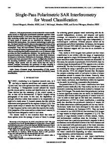
1. Polarimetric Interferometric SAR (POLInSAR) The techniques considered in this paper employ imaging radar interferometry, a dual sensor technology which coherently combines backscatter measurements from two ends of a baseline B, shown as positions 1 and 2 in figure 1 (see [1] for a general review and extensive background references). The sensors are assumed to move in parallel linear trajectories in the x-direction. This enables generation of a synthetic aperture for both sensors and hence high resolution imaging in the range/azimuth or x,z’ plane. By coregistering these two images we can then form the phase difference and obtain a high resolution 2-D image of the variation of interferometric phase in the x,z’ plane. The measurements can either be made by a single platform dual antenna system (single-pass) or by repeat visits of a single antenna system (repeat-pass). The latter suffers from loss of signal coherence due to any temporal changes in the scene between passes. In this paper we ignore such temporal decorrelation effects and concentrate instead on the influence of combined surface and volume scattering. Although interferometry requires the backscatter amplitude to be sufficiently above the system noise level, the key observable of interest is not amplitude but the interferometric phase. This is non-zero due to the slightly different propagation path lengths, Δr, from sensors 1 and 2 to a point on the surface. From the geometry in figure 1and by assuming we both transmit and receive from points 1 and 2, this phase has the form shown in equation 1 (see [1] for a full derivation).

exp(i2kΔr) ≈ exp(i

4 π Δθ

λ

y') ≈ exp(i

4 π Bn y') λR

(1)

where Δθ ≈ Bn/R if R >> B and the co-ordinate y’ is defined as normal to the slant range direction such that y’,z’ define a local orthogonal co-ordinate system as shown in figure 1. Note that the interferometric sensitivity depends only on the normal component of the baseline, Bn, which depends on the absolute baseline B, the baseline orientation angle δ and the angle of incidence θo as defined in figure 1. Transforming Hellmann, M.; Cloude, S.R. (2007) Polarimetric Interferometry – Target Detection Applications. In Radar Polarimetry and Interferometry (pp. 10-1 – 10-22). Educational Notes RTO-EN-SET-081bis, Paper 10. Neuilly-sur-Seine, France: RTO. Available from: http://www.rto.nato.int/abstracts.asp.

RTO-EN-SET-081bis

10 - 1

Form Approved OMB No. 0704-0188

Report Documentation Page

Public reporting burden for the collection of information is estimated to average 1 hour per response, including the time for reviewing instructions, searching existing data sources, gathering and maintaining the data needed, and completing and reviewing the collection of information. Send comments regarding this burden estimate or any other aspect of this collection of information, including suggestions for reducing this burden, to Washington Headquarters Services, Directorate for Information Operations and Reports, 1215 Jefferson Davis Highway, Suite 1204, Arlington VA 22202-4302. Respondents should be aware that notwithstanding any other provision of law, no person shall be subject to a penalty for failing to comply with a collection of information if it does not display a currently valid OMB control number.

1. REPORT DATE

2. REPORT TYPE

01 FEB 2007

N/A

3. DATES COVERED

-

4. TITLE AND SUBTITLE

5a. CONTRACT NUMBER

Polarimetric Interferometry Target Detection Applications

5b. GRANT NUMBER 5c. PROGRAM ELEMENT NUMBER

6. AUTHOR(S)

5d. PROJECT NUMBER 5e. TASK NUMBER 5f. WORK UNIT NUMBER

7. PERFORMING ORGANIZATION NAME(S) AND ADDRESS(ES)

German Aerospace Center (DLR), VO-ST, Linder Höhe, D-51140 Köln, Germany 9. SPONSORING/MONITORING AGENCY NAME(S) AND ADDRESS(ES)

8. PERFORMING ORGANIZATION REPORT NUMBER

10. SPONSOR/MONITOR’S ACRONYM(S) 11. SPONSOR/MONITOR’S REPORT NUMBER(S)

12. DISTRIBUTION/AVAILABILITY STATEMENT

Approved for public release, distribution unlimited 13. SUPPLEMENTARY NOTES

See also ADM001954., The original document contains color images. 14. ABSTRACT 15. SUBJECT TERMS 16. SECURITY CLASSIFICATION OF: a. REPORT

b. ABSTRACT

c. THIS PAGE

unclassified

unclassified

unclassified

17. LIMITATION OF ABSTRACT

18. NUMBER OF PAGES

UU

22

19a. NAME OF RESPONSIBLE PERSON

Standard Form 298 (Rev. 8-98) Prescribed by ANSI Std Z39-18

Polarimetric Interferometry – Target Detection Applications to the surface y,z co-ordinates using the local angle of incidence θ we can also express equation 1 in the modified form exp(i φ(y, z)) as shown in equation 2

⎞ ⎞ ⎛ 2 kBn sin θ ⎛ 2 kBn cos θ + 2 Δk cos θ ⎟ − 2 Δk sin θ ⎟ + z ⎜ ⎠ ⎝ ⎠ ⎝ R R

φ (y, z) = y⎜

Δk =

kBn R tan θ

(2)

Here we have further included the possibility of making a wavenumber shift Δk between the two images [2]. As is apparent from equation 2, we can then always remove the ‘y’ dependence of the phase φ by choosing Δk based on the geometry of the system. In this case the interferometric phase depends only on the height of the scatterer above the reference plane (the z co-ordinate in figure 1). To study any decorrelation in the ‘z’ direction, we then define an effective propagation constant using 1 and 2, as shown in equation 3

kz =

4 π Δθ 4 πB n ≈ λ sin θ λR sin θ

(3)

In foliage examples there will be a random distribution of scatterers in the vertical direction. This causes fluctuations in the phase that are manifest as a drop in the interferometric coherence γ [1]. In polarimetric systems we have 3 channels of complex data at positions 1 and 2 characterised by the elements of the coherent scattering matrix SHH, SVV and SHV [3,4]. In this case the fluctuations can be characterised by a 6 x 6 Hermitian coherency matrix [Θ] as defined in equation 4 [3]. To generate the appropriate coherence we need first to project the channels onto a 3 dimensional complex unitary weight vector w1 to generate a complex scalar s1 as shown in equation 5. Similarly we can define a different weight vector w2 and scalar s2 at position 2. The unitary weight vectors can be parameterised in the form shown in equation 5. Here α is the selected scattering mechanism and β the orientation of that mechanism in the plane of polarisation. Further details of the relationship between w and polarisation parameters can be found in [3,4]. The interferometric coherence for arbitrary polarisation is then defined as the average normalised product of the scalar projections as shown in equation 5 [3]

2 B

δ

δ

B

Bn = B cos(θ0

θo

1

Surfac e

R+Δ + r

Definition of normal baseline component B

R

z z ’

y ’

θ x

y

Figure 1: Radar interferometry and surface geometry. 10 - 2

RTO-EN-SET-081bis

Polarimetric Interferometry – Target Detection Applications

[Θ] =

⎡ k1 ⎤ *T ⎢ ⎥ k1 ⎣k 2 ⎦

[

*T

k2

]

⎧ ⎪⎡ [T11 ] [Ω12 ]⎤ ⎪⎢[Ω ]*T [T ]⎥ 22 ⎦ ⎪⎣ 12 =⎨ ⎪ ⎡ [C ] [Γ ]⎤ 12 ⎪ ⎢ 11*T ⎥ [C22 ]⎦ ⎪ ⎣[Γ12 ] ⎩

⎡S HH + SVV ⎤ 1 ⎢ ⎥ S HH − SVV ⎥ k= ⎢ 2 ⎢⎣ 2S HV ⎥⎦ ⎡ S HH ⎤ ⎢ ⎥ k = ⎢ 2 S HV ⎥ ⎢⎣ SVV ⎥⎦

(4)

Note that the coherence amplitude and phase can be combined and represented as a point inside the unit circle of the complex plane. We see that the coherence and phase can be expressed in terms of 3x3 block elements of the 6 x 6 matrix [Θ]. In equation 4 we have shown two different representations of [Θ] [4]. The coherency form is generated by a Pauli matrix expansion of the symmetric 2 x 2 complex scattering amplitude matrix [S]. This leads to a polarimetric coherency matrix [T] as shown in 5. The covariance matrix [C] follows from a straightforward vectorial expansion of [S]. The two are unitarily equivalent [4] and so have the same eigenvalues but different eigenvectors. We shall make use of both representations in this paper. To evaluate this coherence we now need to estimate the block 3x3 matrices [T] and [Ω].

⎡ cosαe iψ1 ⎤ ⎢ ⎥ w = ⎢sin α cos βe iψ 2 ⎥ ⎢⎣sin α sin βe iψ 3 ⎥⎦

0≤α ≤

π

2 −π < β ≤ π

⇒

⎧ s1s*2 w1*T Ω12 w 2 ⎪γ = = ⎪ s1 = w1*T k1 ⎫ w1*T T11 w1 .w *T s1s1* . s2 s*2 2 T22 w 2 ⎬ ⇒⎨ *T s2 = w 2 k 2 ⎭ ⎪ ⎪ φ = arg( s1s2 * ) = arg w1*T Ω12 w 2 ⎩

(

)

(5)

1.1 The Coherence of Volume Scattering In many vegetation problems, the scatterers in a volume will have some residual orientation correlation due to their natural structure (branches in a tree canopy for example). In this case wave propagation through the volume is characterised by two eigenpolarisations a and b (which we assume are unknown but orthogonal linear polarisations). Only along these eigenpolarisations is the propagation simple, in the sense that the polarisation state does not change with depth into the volume [5]. By assuming that the medium has reflection symmetry about the (unknown) axis of its eigenpolarisations, we obtain a polarimetric coherency matrix [T] and corresponding covariance matrix [C] in the a,b basis for backscatter from the volume as shown in equation 6 [4]

⎡t11 ⎢ [T] = ⎢t12* ⎢⎣ 0

RTO-EN-SET-081bis

t12 t 22 0

0⎤ ⎥ 0⎥ t 33 ⎥⎦

⎡c11 0 c13 ⎤ ⎢ ⎥ [C] = ⎢ 0 c 22 0 ⎥ * ⎢⎣c13 0 c 33⎥⎦

(6)

10 - 3

Polarimetric Interferometry – Target Detection Applications We can now obtain an expression for the matrices [T11] and [Ω12] for an oriented volume extending from z = z0 to z = z0 + hv as vector volume integrals as shown in equations 7 and 8 [5,6] (σ a +σ b )z' ⎧⎪ h ⎫⎪ v ikz z' cosθ o [Ω12 ] = e R(2β )⎨ ∫ 0 e e P (τ ) T P(τ *)dz'⎬ R(−2β ) ⎪⎩ ⎪⎭ ⎧⎪ h (σ a +σ b )z' ⎫⎪ v [T11 ] = R(2β )⎨ ∫ e cosθ o P (τ ) T P(τ *)dz'⎬ R(−2β ) ⎪⎩ 0 ⎪⎭ iφ (z o )

(7)

(8)

where for clarity we have dropped the brackets around matrices inside the integrals and defined the following terms

⎡1 0 0 ⎤ R( β ) = ⎢0 cos β sin β ⎥ ⎢⎣0 − sin β cos β ⎥⎦

⎡cosh τ sinh τ 0 ⎤ P(τ ) T P(τ *) = ⎢ sinh τ cosh τ 0 ⎥ 0 1 ⎥⎦ ⎢⎣ 0

(9)

⎡t11 t12 0 ⎤ ⎢t12* t 22 0 ⎥ ⎢0 0 t ⎥ 33 ⎦ ⎣

⎡cosh τ * sinh τ * 0 ⎤ ⎢ sinh τ * cosh τ * 0 ⎥ ⎢⎣ 0 0 1 ⎥⎦

⎛σ a − σ b ⎞ z' + ik (χ a − χ b )⎟ ⎝ 2 ⎠ cosθ o

(10)

τ =⎜

(11)

Here R is a rotation matrix to allow for mismatch between the radar co-ordinates and the projection of the eigenstates into the polarisation plane. P is a 3 x 3 differential propagation matrix accounting for differential phase (birefringence) and attenuation (dichroism) in the medium via the complex differential propagation constant τ. The waves propagate with extinction σ where σa ≥ σb and refractivities (1-index of refraction) χ [5].This now enables us to generate the coherence for any choice of weight vector w in equation 5. However we are primarily interested in the variability of coherence with changes in w and so employ the coherence optimiser developed in [3], which requires solution of an eigenvalue problem as shown in equation 12.

[T22−1 ] [Ω12]*T [T11−1 ] [Ω12 ] w 2 = λ w 2 ⎫ 2 ⎬ 0 ≤ λ = γ opt ≤ 1 −1 −1 *T [T11 ] [Ω12 ] [T22 ] [Ω12 ] w1 = λ w1 ⎭

(12)

The eigenvalues of these matrices are all real positive and indicate the variability of coherence with polarisation. For example, if the three eigenvalues are equal then the coherence is invariant to polarisation. As the eigenvalues are invariant to unitary transformations of the vector k we can replace [T] by [C] and [Ω] by [Γ] in equation 12. This is important because to account for the effects of propagation on the polarimetric response of an oriented volume, it is simpler to employ the covariance [C] in the a,b basis rather than the coherency matrix [T]. We can then calculate the 3 complex optimum coherence values such that

1 ≥ γ˜1 ≥ γ˜ 2 ≥ γ˜ 3 ≥ 0 as shown in equation 13 (see [6] for details). The key steps involved are to first

convert from [T] to [C] in 12, assume that [C11] = [C22] and then show that [C11]-1 [Γ12] is diagonal in the a,b basis using the analytic expressions in equations 6,7 and 8. The inverse matrix can be easily calculated as a 2 x 2 sub-matrix from the symmetry constraint of equation 6. This then confirms that the maximum coherence

10 - 4

RTO-EN-SET-081bis

Polarimetric Interferometry – Target Detection Applications is always obtained in the a,b basis and evaluation of the corresponding eigenvalues in equation 12 leads to the following expressions for the ranked coherence optima.

1 ≥ γ~1 ≥ γ~2 ≥ γ~3 ≥ 0

γ~1 = f (σ a ) =

h

γ~2 = f (σ a , σ b ) = γ~3 = f (σ b ) =

2σ a z '

v 2σ a e iφ ( zo ) e ik z z ' e cos θ o dz ' ∫ 2σ a hv / cos θ o − 1) 0 cos θ o (e

(σ a + σ b ) e iφ ( z ) o

cos θ o (e

(σ a +σ b ) hv / cos θ o

(σ a +σ b ) z '

hv

e − 1) ∫

ik z z '

e

cos θ o

dz '

(13)

0

2σ b z '

v 2σ b e iφ ( zo ) e ik z z ' e cos θ o dz ' ∫ 2σ b hv / cos θ o − 1) 0 cos θ o (e

h

Equation 13 shows that the maximum coherence is obtained for the medium eigenpolarisation with the highest extinction. This makes physical sense as the polarisation with highest extinction has the minimum penetration into the vegetation and hence the smallest amount of volume decorrelation. Similarly, the lowest coherence is then obtained for the orthogonal polarisation, which has the minumum extinction and hence better penetration into the vegetation and more volume decorrelation. The cross polar channel, which propagates into the volume on one eigenpolarisation and out on the other, has a coherence between these two extremes. Clearly for foliage penetration the lowest extinction is the most useful. If the vegetation cover is strongly oriented then direct use of 13 via the optimisation process in equation 12 can be used to align the radar co-ordinates with the eigenstates and hence select the polarisation that obtains minimum extinction by the vegetation. However in many applications, especially at higher microwave frequencies, forest cover will be random and any orientation effects are likely to be weak [7]. For this reason, to deal with higher frequency problems we must consider a special case of equation 13 when the vegetation shows full azimuthal symmetry in the plane of polarisation [4]. In this case the coherency matrix [T] for the volume is diagonal with 2 degenerate eigenvalues of the form shown in equation 14 [3].

⎡1 0 0⎤ [Tv ] = mv ⎢0 η 0⎥ ⎢⎣0 0 η⎥⎦

0 ≤η ≤1 (14)

where η depends on the mean particle shape in the volume and on the presence of multiple scattering [4]. More importantly, the eigenvalues in equation 13 must become equal. This arises when σα = σβ = σ i.e. when the extinction in the medium becomes independent of polarisation. Figure 2 summarises this special case. Here we show a target covered by a vertical layer of vegetation of thickness hv, inside of which the wave is extinguished by a scalar extinction coefficient σ as shown. It follows from equation 13 that the observed phase fluctuations or coherence for the volume only case is given by equation 15, where Tv is the diagonal polarimetric coherency matrix of the vegetation (equation 14). Here we see a ratio of volume integrals that is independent of polarisation i.e. the observed coherence will be the same for all polarisation channels w. The penetration depth is the same for all polarisations and the fixed phase centre lies somewhere between half the vegetation height and the top as we now show.

RTO-EN-SET-081bis

10 - 5


w

*T

γˆ v =

hv

∫e

2σz' cosθ o

0

w

*T

hv

∫e

e

ikz z'

2σz' cosθ o

hv

TV dz' w =

mv ∫ e

TV dz' w

0

=

0 hv

mv ∫ e

e ikz z' dz'

2σz' cosθ o

dz'

0 hv

2σ cosθ o (e 2σ hv / cosθ o −1)

= f (hv ,σ ) =

2σz' cosθ o

∫e

2σ z' ikz z' cosθ o

e

dz'γ v

0

−1) p1 (e p1 h v p2 (e −1) p 2 hv

⎧ 2σ ⎪⎪ p1 = cosθ o ⎨ σ 2 ⎪ p2 = + ikz ⎪⎩ cosθ o

(15)

In the limit that the extinction σ is zero, equation 15 reduces to the elementary sinc function as shown in 16. This shows that the vegetation layer causes a phase shift or vegetation bias given by half the vegetation height. As the extinction increases, this phase offset moves up in the canopy, until for very high extinction there is no penetration and the vegetation bias equals the vegetation height.

γˆv σ →0 = e

h ikz v 2

⎛k h sin z v ⎞ ⎝ 2 ⎠ k z hv 2

(16)

Note that the phase variance or coherence is also a function of height. As the height increases so the coherence initially drops. Hence in order to obtain a good estimate of the phase we need to employ multilook averaging. The detailed statistics of fluctuations in estimates of phase and coherence were first developed by Lee et al. [8] and further analysed by Touzi et al [11]. However, a simplified analysis provides convenient expressions for the Cramer-Rao bounds on the variance of the estimates as shown in equation 17 [9]

varφ >

1− γ

2

2N γ

2

varγ >

(

1− γ

2N

)

2 2

(17)

Here N is the equivalent number of looks in the averaging process. We see that as N increases so the variance of the estimates decreases and that the phase variance increases with decreasing coherence. We conclude from this analysis that if orientation effects are present in vegetation cover then polarimetric interferometry can exploit this to select a channel with the minimum extinction and hence achieve optimum foliage penetration. This maximum penetration channel corresponds to the minimum eigenvalue of the coherence optimiser. However, to counter this we have seen that when the vegetation becomes random then the extinction no longer varies with polarisation. In this case we seem to have no choice but to employ a longer wavelength that leads to a low extinction. However, by exploiting the polarimetric sensitivity of interferometric coherence to the presence of a target beneath the random vegetation, we can offset this requirement to achieve significant sub-clutter visibility as we now show.

10 - 6

RTO-EN-SET-081bis


2. Two-Layer Vegetation Model for Target Detection In the previous section we considered the vegetation layer alone. Here we extend the analysis to consider a 2 –layer problem consisting of a random vegetation layer above a localised scattering centre, which acts as a model for a vehicle or other target beneath the canopy [7,10]. Figure 2 shows the geometry to be considered. We assume homogeneity in the y-direction and so consider only z or height variations. In this way the problem can be specified by a 1-dimensional vertical profile function d(z) as shown. The vegetation is modelled as a random volume with scalar extinction σ. The target is located at some unknown depth zo and has an apparent magnitude mg. Note that the azimuthal symmetry assumption applies only to the vegetation layer and that the target can have arbitrary form (including rotations due to sloped terrain/target orientation etc.). The observed coherence must now be modified from equation 15 to account for the presence of the target. This we can do as shown in equation 18, where the angles φ and φ2 are the phase centres of the target and bottom of vegetation layer respectively.

T11 = I + e V 1

I =e V 1

−

2σh v cosθ o G 1

−

iφ 2 V 2

Ω12 = e I + e e

I

2σh v h v cosθ

∫e

2σz' cosθ o

I = G 1

TV dz'

0

I =e V 2

−

2σh v h v cosθ

∫e

iφ 1

hv

−

∫ δ(z')e

2σh v cosθ o G 2

2σz' cosθ o

I

Tg dz' = Tg

0 2σz' cosθ o

e ikz z'TV dz'

I2G = Tg (18)

0

Collecting terms we can write the coherence as shown in equation 19, which also shows explicitly the polarisation dependence of the total observed coherence. *T

γ˜ =

−

2σh v cosθ o

−

2σh v cosθ o

w (e iφ 2 I2V + e *T

w (I + e v −1 =

V 1

Tg e iφ1 )w

w (e iφ 2 v −1I2V + e iφ1 v −1Tg )w *T

=

1+ w *T v −1Tg w

Tg )w

1 w I w *T V 1

γˆ (w ) = e iφ

1

⎞ γˆ v + μ(w ) iφ ⎛ μ(w) = e ⎜ γˆ v + (1− γˆ v )⎟ 1+ μ(w) 1+ μ(w) ⎝ ⎠ 1

= e iφ1 (γˆ v + L(w )(1− γˆ v ))

0 ≤ L(w) ≤ 1

(19)

The parameter μ is the target-to-volume scattering ratio and is defined in equation 20 *T

2σ

μ(w ) =

cos θo (e

2σh v cosθ 0

− 1)

w Tg w w *T TV w

≥0 (20)

Since both T matrices in equation 20 are Hermitian, it follows that μ is a positive semi-definite function. We see that the presence of a target beneath the canopy influences the observed coherence. If the target scattering changes with polarisation then this will be reflected in changes in the observed coherence. Hence by using polarimetric interferometry we can detect the presence of targets by looking at the variation of coherence with polarisation. For vegetation only this will yield zero or small changes, however bright the

RTO-EN-SET-081bis

10 - 7

Polarimetric Interferometry – Target Detection Applications canopy return. However, when a target is present the changes will be larger hence enabling sub-clutter visibility of targets. We note from equation 19 that we can write the coherence in terms of a real function L that varies from 0 to 1. This defines a line in the complex plane inside the unit circle [10]. Figure 3 shows a geometrical representation of this line. We see that by measuring the coherence and relating it to the end points we can estimate μ the ground-to-volume scattering ratio for that polarisation. The red (left) point is the μ=0 or volume coherence alone. This we can approximate by measuring the coherence in a channel with smallexpected target signal, the cross-polarised HV channel for example. The yellow (right) point is the bare earth topography and is not directly visible in the data because of the vegetation cover. However by extrapolating the line beyond its visible length we can estimate the bare earth topography from the unit circle intersection [10].

γˆ v e iφ − γˆ (w) μ(w) = γˆ (w ) − e iφ 1

1

γ˜ ve iφ

1

γ˜(w)

e iφ 1 Unit circle of complex coherence

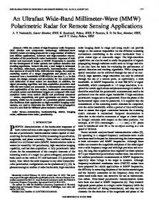
Figure 3: The line coherence model for target+random volume scattering Note that we obtain an ambiguity with this method as there will be two such intersection points, only one of which will correspond to the true ground topography. This can be resolved using rank ordering of coherence or a reference digital terrain model (DTM) for the scene [10]. Having identified a mechanism by which targets can be detected, we now investigate the sensitivity of the method to the presence of target scattering. To do this we calculate the derivative of coherence with respect to the target-to-volume ratio as shown in equation 21

∂γˆ (1− γˆv ) = = f (μ)g(γˆ v ) ∂μ (1+ μ)2

(21)

We are particularly interested in the case where μ is less than 1, this being a situation where the volume scattering is larger than that from the target. Equation 21 is the product of 2 terms. Concentrating first on the μ dependence, we can express this sensitivity by calculating the function L in equation 19, being the fractional change in the length of the line due to a presence of a target. We see that even with –10dB of 10 - 8

RTO-EN-SET-081bis

Polarimetric Interferometry – Target Detection Applications scattering ratio, the shift in coherence is about 10% of the line length. The line length itself is 1− γ v . Hence in order to be able to detect a small change we need to choose the baseline so that the length is maximised. This would seem to require that γv = -1 i.e. the baseline is chosen so that the vegetation phase centre lies at the π height. However this must also occur with a coherence magnitude of unity. Examination of equation 15 shows that this requires infinite extinction in the medium. Clearly this is not a practical solution and hence in practice the optimum baseline will be a function of both height and wave extinction. As an example, figure 4 shows how the line length varies with increasing kz for typical values of 10m high trees and 0.3 dB/m one way extinction. Note that the line length (in red) increases to a maximum before decreasing again and then shows oscillatory behaviour.

ˆ

1.6

1.4

maximum line 1

m

L (red) and gamma in (blue)

1.2

Optimum i

0.8

0.6 Height = 10m, sigma = 0.3 dB/m 0.4

minimum line

0.2

0

0

0.1

0.2

0.3

0.4

0.5 kz

0.6

0.7

0.8

0.9

1

Figure 4: Line length variation with increasing baseline and minimum coherence along the line. The intersection point represents a compromise between sensitivity and resolution. There is one additional feature that bears on this question of optimum line length, namely the need to estimate complex coherence from the data itself. There are two issues, the first is the need for a large effective number of looks when the coherence is low. This follows from the Cramer Rao bounds in equation 17. If the coherence line goes through the origin for example then the phase becomes indeterminate. The need for a high effective number of looks (ENL) is serious because it impacts on the resolution requirements of the sensor and also leads to a reduced μ value. This arises since, for point targets, the volume clutter increases with the ENL while the target RCS does not. Hence we need to minimise the ENL and so maximise the minimum line coherence value. The second issue relates to the fact that coherence techniques based on standard box-car averaging provide biased estimates at low coherence [11]. While this bias reduces with increasing coherence and number of looks it tends to overestimate low values of coherence. This is serious as it will give a radial bias to low coherence values and hence distort the line parameter estimates. To solve this we must either use unbiased coherence techniques or set a lower limit (set by the ENL) on the minimum line coherence. In either case we seek to maximise the minimum line distance from the origin. By itself this leads us to choose a zero baseline, as then all coherences are 1. However, when combined with the need to maximise L it leads us to a compromise optimum baseline. This minimum line coherence is shown in blue in figure 4.

RTO-EN-SET-081bis

10 - 9

Polarimetric Interferometry – Target Detection Applications We see that the two curves intersect at one point. This is the optimum for that configuration. It combines good sensitivity to target scattering and also minimises the ENL required for good estimates. In this case we obtain a kz value around 0.15. In general it will be a function of height and extinction. Global mean tree heights lie around 20m and this leads to a rough interferometer design figure of kz = 0.1. The most important factor in determining the best baseline is the tree height. It should be pointed out that this parameter can itself be estimated from the data using polarimetric interferometry techniques [7,10] and hence the optimum baseline can in principle be adapted ‘in the field’ to match local conditions. Our proposed POLINSAR target detection algorithm is then based on estimation of a scalar radar parameter μ, obtained from complex interferometric coherence estimates in different polarisation channels w. The parameter μ is dimensionless, being the ratio of all scattered power contributions with an apparent phase centre located on the surface, to the total volume scattering. The former includes direct surface returns, the desired target backscatter as well as dihedral effects caused by specular surface scattering and secondary interactions with the vegetation (ground-trunk returns). The volume returns include all scattering (single and multiple) with phase centres displaced from the surface. It follows from this that the presence of a target corresponds to a local maximum in μ. Further, from the conventional SAR intensity channel we obtain an estimate of the sum of these two contributions s(w) as shown in equation 22.

cos θ o (1− e s(w) = 2σ

−

2σh v cosθ 0

)

*T

w TV w + e

−

2σh v cosθ 0

*T

w Tg w

(22)

Hence we can solve equations 20 and 22 to obtain an estimate of the surface scattering components as shown in equation 23 *T

w Tg w = e =e

2σh v cosθ 0

2σh v cosθ 0

μ(w) s(w) 1+ μ(w)

L(w )s(w) = e

2σh v cosθ 0

F(w) 0 ≤ L(w) ≤ 1

(23)

The function L(w) acts as a filter on the intensity channel to produce an image domain with better signal to clutter ratio. Note that because we always see the ground components through the canopy, they are influenced by the local extinction and height of the vegetation as shown in 23. However, all ratios between polarisation channels (such as HH/VV etc.) are independent of height and extinction (under the assumption of a random volume). This is important for target classification studies. Using the above results we can now devise a general algorithm for target detection using polarimetric interferometry.

3. POLINSAR Target Detection Algorithm We assume access to two single look complex fully polarimetric SAR images that have been co-registered and phase and amplitude calibrated. We also assume that there are no temporal decorrelation or signal to noise ratio problems in the data. We then propose a generic processing chain as follows: Stage 1 : Coherence Estimation The first stage is to generate complex coherence estimates for a number of polarisation states w. In all cases, equation 5 is used with the appropriate w vectors. For simplicity we adopt a boxcar averaging process for coherence estimation, employing an M x M window centred on the pixel of interest. However we must realise that this will lead to coherence bias for low coherence values, as discussed in [11]. It will also lead to edge effects on the boundaries between different scatterer types, when the true coherence will be 10 - 10

RTO-EN-SET-081bis

Polarimetric Interferometry – Target Detection Applications underestimated because of mixed scattering mechanisms. Here we ignore such effects but note that forest edges are of significant tactical importance in hidden target applications. Initial development of coherence estimators that are more suitable for such problems are presented in [12]. Stage 2 : Least Squares Line Fit The next stage is to find the best-fit straight line to the polarimetric coherence values inside the unit circle (using a reference DTM if available to fix the unit circle intersection point). From these line parameters we then project each of the measured complex coherence values γi onto the least squares line. This projection then ensures real μ estimates as required in equation 20. Stage 3 : Select the reference volume coherence channel For single baseline systems we cannot estimate the volume coherence point uniquely [10]. There are a set of candidate volume coherence values defined geometrically as all points on the line which lead to an observed positive semi-definite function μ(ω). Nonetheless, in practice we can select a polarisation channel we expect to be close to the true volume point. Often this will just be the cross polar HV channel, where we expect a small target-to-clutter ratio in most cases. In this study we employ the HV channel throughout. A more general strategy is to employ the polarisation with maximum vegetation bias [10]. Stage 4 : Estimate Ground Scattering Components and Filtered Intensity Having estimated the extreme points on the coherence line, we can now estimate the μ value in any desired polarisation channel. Figure 5 shows how we can estimate these two values for the HH+VV and HH-VV channels matched respectively to trihedral and dihedral scatterers. Here we show two cases, background clutter (lower) and the presence of a target (upper). From μ we can then obtain L(w) using equation 19. We then estimate the mean backscatter intensity in the w channel using a the same boxcar average as for the coherence and finally multiply this intensity by the function L to obtain F(w).

μ••••• μ•••••

Target present

γˆ HV

γˆ HH −VV

γˆ HH +VV No target

e iφ 1 L(w) =

μ(w ) 1+ μ(w )

e iφ 1

Figure 5: Polarimetric target-to-volume scattering ratio estimation. To quantify the potential of this method to suppress forest clutter and provide enhanced detection, we now turn to consider its application to simulated POLINSAR data.

RTO-EN-SET-081bis

10 - 11


4. POLINSAR Target Simulations To enable an assessment of algorithm performance, a Maxwell equation based wave propagation and scattering model is used to generate test image data for trihedral and dihedral corner reflectors embedded in foliage clutter. Several approaches to the modelling of coherent forest microwave scattering have been developed in the literature [13-17]. Our simulation employs a 3-D voxel-based, vector wave propagation and scattering model coupled to a detailed description of tree architecture and forest structure [15-17]. The SAR simulation is fully polarimetric, coherent and deterministic, and so may be used to model volume decorrelation effects, as required in polarimetric SAR interferometry. Simulation of the SAR images is a multistage process that begins with the construction of a detailed computer model of the scene to be imaged. This model incorporates a digital terrain map (DTM) of the underlying surface (generated artificially or supplied from observation), and soil description parameters including local roughness, correlation length, soil type [18] and moisture content. A map of tree heights and locations is calculated that corresponds closely to observed distributions [16], the stand density employed here being moderate at 0.055 stems/m2, with a mean height of 18m and height standard deviation of 0.6m. The forest canopy is populated with Scots Pine tree models in the form of collections of layered, dielectric cylinders calculated according to biologically determined growth rules [15]. The tree models are architecturally correct (see Figure 6.) and include details of the size and distribution of pine needles along living branches. The water contents of deadwood, sapwood, heartwood and pine needles [16] complete the physical description of the forest canopy. Finally, targets, modelled as collections of perfectly conducting, interacting surfaces, are positioned throughout the scene. Modelled in this fashion, the forest canopy represents a distribution of discrete, dielectric objects. As such L-Band scattering by the canopy may be calculated using the mean-field approach pioneered by R H Lang [19, 20], and subsequently extended to layer geometry and employed in backscatter modelling of grass canopies [21] and of forest canopies at Cband [22]. The mean–field approach is a coherent wave model that approximates the locally incident field at any discrete scattering object by the mean wave propagating in the layer, and calculates scattering using a Green’s function for the mean wave. For a homogeneous medium the Green’s function for the mean wave is everywhere the same. However the forest canopy is inhomogeneous on a scale commensurate with the resolution of the SAR system and it is desirable to incorporate the effects of canopy inhomogeneity into the simulation. In this way targets deployed so as to be visible to the SAR sensor through gaps in the canopy will not appear attenuated by some global mean attenuation constant. To achieve this we employ the form of the layered Green’s function of the mean wave [20,21], but estimate the wavenumber of the mean wave locally for the aperture used to focus each scattering interaction. In practice this entails dividing the canopy volume into sub-volumes (voxels) on a scale determined by the sensor resolution, and such that each voxel contains a large number of scattering objects. The detailed forest model is used to determine the occupancy of each voxel, and then effective permittivity of the voxel is calculated using the Foldy-Lax approximation [21, 22] with vegetation permittivities determined using the model described in [24] at frequencies used by the SAR instrument. Tree branches are divided into many elements in order to better estimate voxel volume fractions. To calculate backscatter from any element of the scene the effective wavenumber is determined using the mean properties of voxels intercepted by the line of sight between the current sensor position and the scene element. The dependence of the effective wavenumber, and hence of the attenuation of scattering amplitudes, both upon frequency and polarisation, arises naturally in the model from the physical and biophysical descriptions. SAR is a coherent imaging process, and thus the mean field model is an appropriate model to adopt in the simulation. Scattering of the coherent, mean wave is focused by the SAR instrument using the phase history of the scattered signal [25]. Coherent phase histories are modelled in the simulation, but the contribution to the image from scattering of the incoherent wave is not modelled directly. This may be incorporated in the form of a noise signature. Calculation of simulated SAR images proceeds by forming the coherent superposition of focused scattering events, each arising from a scene element much smaller than the SAR system resolution. The simulated SAR image may be described as

P ( x0 , R0 ) = ∑ F j Qˆ ( x0 , R0 , s j ) j

10 - 12

(24) RTO-EN-SET-081bis


where

P ( x0 , R0 ) is the polarimetric pixel value at cross range x0 and range R0 , F j is the polarimetric Qˆ ( x0 , R0 , s j )

scattering amplitude associated with the scene element, and

is the complex system point

s

F

j may be spread function depending upon the effective scattering centre j . Scattering amplitudes calculated as averages both in azimuth (along the synthetic aperture) and frequency (across the SAR

ˆ

bandwidth). The system point spread function Q is determined from the specified SAR imaging geometry, bandwidth and processing options. The platform motion is ideal, and the platform is modelled as having a straight, uniform trajectory. Each scene element has an effective scattering centre, which determines the point of focus of backscatter in the two dimensional SAR image. For first order or direct backscatter the effective scattering centre is simply the centre of the scene element. For higher order returns, involving multiple reflections, the effective scattering centre is determined rapidly at run-time using knowledge of the scattering path and the antenna motion. The centre of focus in the SAR image is simply the projection of the effective scattering centre onto the SAR imaging plane, which may be calculated using near-field or far-field models. Simulated single-look, complex SAR images are output in ground range and azimuth. Direct-ground contributions are calculated from ground facet elements using a hybrid deterministic/stochastic approach. Ground facet RCS values depend on local incidence through a physical scattering model (the Bragg or small perturbation model), to which speckle is added. Local speckle statistics are assumed Gaussian and scattering amplitude values are drawn from distributions using the mean RCS for the facet as determined from local incidence. A spatially correlated speckle phase model may be used which depends upon surface roughness, surface correlation length, wavelength and incidence angle. The correlated speckle phase model reduces to spatially uncorrelated speckle phase for short wavelength and surface correlation length, as well as for large surface roughness. To calculate direct forest clutter, each branch element is addressed in turn with scattering amplitudes calculated using the mean field and truncated, infinite cylinder approximations [26]. No calculation of multi-path between tree elements is performed since this has in theory already been taken into account in the mean-field model. We note however that for correct calculation of cross-polar returns at higher frequencies than L-band the explicit incorporation of such multiple interactions may be necessary [27]. Needle scattering is estimated in a statistical manner, by simulating short random walks using a generalised Rayleigh-Gans scattering model for needles [28], and scaling these short walks depending upon the number of needles associated with each branch element. In general the ground has arbitrary roughness and many different scales of variation in height. Calculations are limited to the case that the ground may be assumed locally flat, but roughened and tilted. Local orientation of the mean surface for ground-element interactions is calculated from the mean slope close to the scattering element. Ground-element interactions have effective scattering centres located as the normal projection of the true scattering centre in the locally flat, mean surface. Similarly, ground-element-ground interactions have effective centres located at the reflection of the element centre in the locally flat, mean surface. Targets are modelled as collections of perfectly conducting surfaces. Each of the target surfaces is divided into triangular facets of dimension much less than the system resolution. Multipath scattering amplitudes are calculated for each facet in the final surface of a multipath scattering chain using the geometrical optics, and physical optics approximations [29]. This model yields accurate RCS estimates, and preserves the expected polarimetric responses of known targets types. The effective scattering centre for each such surface facet is calculated by tracing the history of the specular path of a multipath event during formation of the synthetic aperture. This approximation is consistent with the geometrical optics model used for all but the last scattering interaction in any surface scattering chain. Interactions involving up to three surfaces are considered in the calculations, which include surface shadowing effects [17]. The method of specular path tracing lends itself readily to the modelling of multipath between ground and target when the ground is essentially locally flat (over the region traversed by the specular point) and only slightly rough: the ground acts as a primary reflecting surface in the multipath chain. Ground and target surfaces are distinguished only by their reflection properties: the ground is modelled as a rough dielectric surface, with Fresnel reflection RTO-EN-SET-081bis

10 - 13

Polarimetric Interferometry – Target Detection Applications coefficients scaled according to the surface roughness using the Rayleigh roughness parameter [30]. Effective scattering centres for direct-element, ground-element and ground-element-ground interactions lie respectively above, close-to and below the ground surface. Thus a simulated SAR image of a forest contains a direct-canopy image, displaying layover of tree direct reflectivity towards the radar, a ground-canopy image displaying projection of the ground-tree reflectivity onto the local mean ground surface, and a groundcanopy-ground image displaying layover away from the radar. At L-band the ground-canopy and directcanopy terms appear to influence most strongly the total clutter level and the ground-canopy-ground terms are negligible. Predictions for forest clutter at L-band at 45 degrees elevation of –4dB (HH) –11dB (HV) and –8dB (VV) are consistent with those reported in the open literature for similar forests [31].

5. Simulation Results Figure 6 shows model detail of a single tree (on the left) and an optical view of the entire pine forest scene to be simulated (on the right). Embedded in this scene is an array of 27 square corner reflectors. They are a mixture of trihedrals and dihedrals at two orientation angles, namely 0o and 22.5o, the latter guaranteeing a strong cross-polar response. The details of the target array are shown in figure 7. Three sizes of reflector are used, 90, 60 and 30cm. In this way we model a range of different target responses in both polarization and radar cross section. The spacing between targets is 14m.

Figure 6: Detail of an individual tree drawn without needles (left) and view from aperture centre of the simulated forest stand (150m x 150m) with hidden in-situ corner reflector array (right).

10 - 14

RTO-EN-SET-081bis


Figure 7: Details of the corner reflector array: TXX is a trihedral of dimension XX cm, DVXX is a vertical dihedral, DRXX is a dihedral rotated at 22.5 degrees. The targets are shown with exaggerated dimensions for clarity. We model the radar response at L-band or 23cm wavelength. Analysis of the model with and without vegetation in place then enables estimation of the mean wave extinction σ. For V polarization this corresponds to a 1-way attenuation rate of 0.28 dB/m while for H polarization the extinction is lower, with a mean value around 0.14 dB/m. Hence the model predicts some departure from the azimuthal symmetry assumption required for the FOPEN algorithm. We found however that the algorithm is fairly robust to such levels of differential extinction, although they do seem to act in limiting detection of the smaller targets (see figure 10). Future studies and field experiments will investigate the effects of differential extinction in more detail. For validation reasons, we start with a system configuration closely matched to the DLR E-SAR airborne Lband system [7], which typically operates at an altitude of 3km with a 45-degree angle of incidence in the centre of the swath. The transmitted bandwidth is 100 MHz and the synthetic aperture yields an azimuth resolution around 0.75m. We simulate these conditions to obtain an effective sensor resolution of 1.38m in ground range and 0.69m in azimuth. The data is then over-sampled to obtain a square pixel size of 0.5m. Figure 8 shows simulated L-band SAR imagery for this scene. Four images are shown, corresponding to the four transmitter/receiver polarization combinations. We note that it is difficult to see the corner reflectors in the background foliage clutter, although for example in the cross-polar channel some of the rotated dihedrals can be seen. Figure 9 shows the single look interferometric phase for this scene. In the upper portion we show the raw phase and in the lower the residual phase following flat earth removal of the spatial frequency variation in range due to changes of the angular separation of the antennas for a flat earth geometry. We see that the local topography is relatively flat with the presence of the trees causing volume decorrelation or increased

RTO-EN-SET-081bis

10 - 15

Polarimetric Interferometry – Target Detection Applications phase variance. Again in this single channel interferogram (the VV Channel) there is no clear indication of the presence of targets. It is only when we combine many such interferograms at different polarizations that we can detect the targets more clearly as modulations in the mean phase and variance. We now apply the processing algorithm of section 4 to interferograms in 2 channels, namely HH+VV and HV.

Figure 8: Simulated L-Band, polarimetric SAR Images of the corner reflector array deployed in the model forest. To illustrate the level of processing gain achievable with multi-channel interferometry, we show in figure 10 a comparison of the unfiltered image intensity (using a 5 x 5 window) and the POLINSAR filtered intensity F(w). In both cases we display a dynamic range of 25dB of the peak signal in the scene. In this way we can quickly visualize any signal processing improvements. We have selected the HH+VV polarization channel corresponding to w = (1,0,0), which is matched to the presence of trihedral corner reflectors and so show only the portion of the image around the cluster of TXX targets in figure 7. By changing w we can select different target types in the scene but here we concentrate on the results for the trihedral reflectors only. We can see that the large trihedrals (T90) are seen both in the raw and filtered intensity data but the T60 and T30 reflectors cannot be easily discriminated from the background clutter in the standard intensity channel. The filtered image however shows a strong reduction of the background clutter, allowing both the T90 and T60 reflectors to be much more clearly seen. We note that the T30 reflectors still cannot be detected. The reason for this can be traced to the values for the three target types. We can obtain estimates of μ directly from the separate simulation of target and volume components in the SAR simulator. This analysis shows that T90 has μ = 5 dB, T60 has μ = -2dB and T30 μ = -10 dB. Analysis of residual orientation and structural 10 - 16

RTO-EN-SET-081bis

Polarimetric Interferometry – Target Detection Applications effects in the forest canopy also indicate a maximum filter suppression of –10dB. This explains the poor detection of T30 in this environment. However, despite this, we note that the T60 elements are now much more clearly discriminated from their background. The impact of this on detection statistics is demonstrated in figure 11. Here we show 3-D images of the raw and filtered SAR channels. In the raw channel we see that the 60cm reflectors are obscured by background clutter, leading to a large number of false alarms in the detection process. In the filtered channel on the other hand we can see that the algorithm has suppressed the clutter while maintaining the signal from the target. In the case of the 60cm reflectors, setting a threshold of -3dB their peak value now obtains zero false alarms in the scene. We conclude that the POLINSAR processing gains are significant and warrant further studies of more complex vehicle targets embedded in forest clutter. We also plan further analysis of coherent random vector wave propagation and scattering effects in different forest environments to obtain a more robust assessment of algorithm performance.

Figure 9: Interferometric phase (upper) and residual phase following flat earth removal (lower) for forested scene.

RTO-EN-SET-081bis

10 - 17


Figure 10: Multi-look intensity (upper) and filtered intensity (lower) images of trihedral corner targets in foliage (5 x 5 window, HH+VV channel).

10 - 18

RTO-EN-SET-081bis


Figure 11: Normalised backscatter of trihedral sub-array for unfiltered HH+VV channel (upper) and POLINSAR filter output (lower)

RTO-EN-SET-081bis

10 - 19


6. Conclusions In this section we have introduced the idea of combining multiple interferograms at different polarizations to enhance the detection of targets hidden by foliage. In the case where there are strong orientation effects in the volume scattering we have shown that the coherence optimizer can be used to select the polarization with minimum extinction and hence optimum penetration of the foliage. In the extreme case of random volume scattering, we have shown that we can design a filter based on the invariance of volume decorrelation to polarization state. The presence of a target beneath the volume then breaks this symmetry and leads to a linear variation of coherence inside the unit circle of the complex plane. By normalizing this variation to the distance between the ground topography unit circle and invariant volume decorrelation points, we can generate a filter with range 0 to 1. This filter then multiplies the intensity channel so that in regions where there is volume scattering only the intensity is reduced to zero while the target response is maintained. In this way the target to clutter ratio can be improved and targets detected using a threshold based on conventional constant false alarm rate (CFAR) techniques, applied now to the filtered intensity channel We have illustrated the application of this method to data generated by a full vector wave based SAR simulator which takes as its input detailed three dimensional forest structural and target information, as well as details of the SAR point spread function and generates as output the complex SAR data which accounts for the phase of each scattering element in the scene. In this way the simulator can be used to model volume decorrelation as a function of polarization. We have made simulations of high resolution SAR imagery at 23cm wavelength (L-band) of a pine forest scene containing an array of corner reflectors of different sizes and orientations. In this paper we have concentrated on detection of a cluster of 9 trihedral reflectors and have shown significant improvements in detection performance. This suggests the possibility of enhanced target detection in foliage at the relatively high L-band frequency, which has many advantages in the future deployment of space and air borne systems. Future studies will address the detection of more complex target types such as vehicles and issues relating to improved sensor resolution.

7. Acknowledgements The biologically accurate tree architectural models for Scots Pine used in this work have been provided by Prof. Seppo Kellomäki and Dr Veli-Pekka Ikonen of the Faculty of Forestry, University of Joensuu, Finland. The authors wish to express their sincere gratitude for this data, without which much of this work would not have been possible. Special thanks are also due to Dr Terhikki Manninen, and Dr Tuomas Häme of VTT, Finland, for their continued help and support, and also to Risto Sievänen and Mika Lehtonen of the Finnish Forestry Research Institute, and to Eero Nikinmaa and Timo Vesala of the University of Helsinki, Dept. of Forest Ecology whose expert knowledge has provided guidance in the choice of forest bio-physical parameters. This work has been funded in part both by the UK MOD Corporate Research Programme under project 09/03/01/019/2001, and by the Defence Science and Technology Organisation of Australia.

8. References [1] Bamler R, P. Hartl, 1998, “Synthetic Aperture Radar Interferometry”, Inverse Problems, 14,R1-R54 [2] Gatelli F A Monti Guarnieri, F Parizzi, P Pasquali, C Prati, F Rocca, “The Wavenumber Shift in SAR Interferometry”, IEEE Transactions on Geoscience and Remote Sensing. GRS-32, pp 855-865, July 1994 [3] Cloude S.R., K P Papathanassiou, “Polarimetric SAR Interferometry”, IEEE Transactions on Geoscience and Remote Sensing, Vol 36. No. 5, pp 1551-1565, September 1998 [4] Cloude S.R., E. Pottier, "A Review of Target Decomposition Theorems in Radar Polarimetry", IEEE Transactions on Geoscience and Remote Sensing, Vol. 34 No. 2, pp 498-518, March 1996

10 - 20

RTO-EN-SET-081bis

Polarimetric Interferometry – Target Detection Applications [5] Treuhaft R.N. , S.R. Cloude,“The Structure of Oriented Vegetation from Polarimetric Interferometry”, IEEE Transactions Geoscience and Remote Sensing, Vol 37/2, No. 5, p 2620-2624, September 1999 [6] Cloude S. R., K.P. Papathanassiou, W.M. Boerner, “The Remote Sensing of Oriented Volume Scattering Using Polarimetric Radar Interferometry”, Proceedings of International Symposium on Antennas and Propagation, ISAP 2000, Fukuoka, Japan, pp 549-552, August 2000 [7] Papathanassiou K.P., S.R. Cloude, “Single Baseline Polarimetric SAR Interferometry”, IEEE Transactions Geoscience and Remote Sensing, Vol 39/11, pp 2352-2363, November 2001 [8] Lee J S, K W Hoppel, S A Mango, A Miller, “Intensity and Phase Statistics of Multi-Look Polarimetric and Interferometric SAR Imagery”, IEEE Trans GE-32, pp. 1017-1028, 1994 [9] Seymour S., Cumming I.G., “Maximum Likelihood Estimation for SAR Interferometry”, Proceedings of IEEE International Geoscience and Remote Sensing Symposium (IGARSS94), Pasadena, USA, 1994 [10] Cloude S.R. , K.P. Papathanassiou, “ A 3-Stage Inversion Process for Polarimetric SAR Interferometry”, IEE Proceedings, Radar, Sonar and Navigation, Volume 150, Issue 03, pp 125-134, June 2003 [11] Touzi R, Lopes A., Bruniquel J, Vachon P.W., “Coherence Estimation for SAR Imagery”, IEEE Transactions Geoscience and Remote Sensing, VOL. GRS-37, pp 135-149, January 1999 [12] Lee J.S., S.R. Cloude, K.P. Papathanassiou, M.R. Grunes, I. H. Woodhouse, “Speckle Filtering and Coherence Estimation of POLInSAR Data for Forest Applications”, IEEE Transactions on Geoscience and Remote Sensing, Vol. 41, No. 10, pp 2254-2263, October 2003 [13] Lin Y.C. , K. Sarabandi, “A Monte-Carlo coherent scattering model for forest canopies using fractal generated trees”, IEEE Transactions Geoscience and Remote Sensing, VOL. GRS-37, pp 440-451, January 1999 [14] Sarabandi K., J.C. Lin “Simulation of Interferometric SAR response for characterising the scattering phase centre statistics of forest canopies”, IEEE Transactions Geoscience and Remote Sensing, VOL. GRS38, pp 115-125, January 2000 [15] Kellomäki S., Veli-Pekka Ikonen, Heli Peltola and Taneli Kolström, “Modelling the Structural Growth of Scots Pine with Implications for Wood Quality”, Ecological Modelling, 122, pp117-134, 1999. [16] Williams M.L., T Manninen, Seppo Kellomäki, Veli-Pekka Ikonen, Risto Sievänen, Mika Lehtonen, Eero Nikinmaa and Timo Vesala, “Modelling the SAR Response of Pine Forests in Southern Finland”, Proceedings of IEEE International Geoscience and Remote Sensing Symposium (IGARSS03), Toulouse, France, Vol II, 1350-1352, July 2003. [17] Williams M.L. and N Harris, “Demonstration of Reduced False Alarm Rates using Simulated L-Band Polarimetric SAR Imagery of Concealed Targets”, Proceedings of the IEEE International Conference on Radar, pp535-540, Adelaide, Australia, September 2003. [18] Dobson M.C., F T Ulaby, M Hallikainen and M El-Rayes, “Microwave Dielectric Behaviour of Wet Soil: Part II: Four-Component Dielectric Mixing Models”, IEEE Transactions on Geoscience and Remote Sensing, vol. GRS-23, pp 35-46, 1985. [19] Lang R.H., “Electromagnetic Scattering from a Sparse Distribution of Lossy Dielectric Scatterers”, Radio Science, vol. 16, pp. 15-30, 1981.

RTO-EN-SET-081bis

10 - 21

Polarimetric Interferometry – Target Detection Applications [20] Lang R.H. and J S Sidhu, “Electromagnetic Scattering froma Layer of Vegetation: A Discrete Approach”, IEEE Transactions on Geoscience and Remote Sensing, vol. 21, pp. 62-71, 1983 [21] Saatchi S.S., D M LeVine and R H Lang, “A Microwave Backscattering and Emmission Model for Grass Canopies”, IEEE Transactions on Geoscience and Remote Sensing, vol. 32, #1, pp. 177-186, 1994. [22] Williams M.L., S Quegan and D Blacknell, “Distribution of Backscattered Intensity in the Distyorted Born Approximation: Application to C-band SAR Images of Woodland”, Waves in Random Media, vol. 7, pp. 643-660, 1997. [23] Frisch U., “Wave Propagation in Random Media”, in “Probabilistic Methods in Aplpied Mathematics”, vol. 1, Ed. A T Bharrucha-Reid (New York: Academic), 1968. [24] Ulaby F.T. and M A El-Rayes, “Microwave Dielectric Spectrum of Vegetation-PartII: Dual-Dispersion Model”, IEEE Transactions on Geoscience and Remote Sensing, GE-25, pp 550-557, 1987. [25] Carrara W.G. , R S Goodman and R M Majewski, “Spotlight Synthetic Aperture Radar Signal Processing Algorithms”, Artech House (Boston, London), 1995. [26] Karam M.A. and A K Fung, “Electromagnetic Scattering from A Layer of Finite, Randomly Oriented, Dielectric, Circular Cylinders Overa Rough Interface with Application to Vegetation”, Radio Science, vol. 18, pp. 557-563, 1983. [27] Williams M.L. and S Quegan, “Modelling Microwave Backscatter from Discrete Random Media using a Multiple-Scattering Series: Convergence Issues”, Waves in Random Media, vol. 7, pp. 213-227, 1997. [28] Schiffer R. and K O Thielheim, Journal of Applied Physics, vol. 50, pp. 2476-2483, 1979. [29] Griesser T. and C A Balanis, “Backscatter Analysis of Dihedral Corner Reflectors using Physical Optics and the Physical Theory of Diffraction”, IEEE Transactions on Antennas and Propagation, vol. AP-35, #10, pp 1137-1147, 1987. [30] Ogilvy J.A. , “Theory of Scattering from Random Rough Surfaces”, IOP Publishing, Bristol and Philadelphia, 1991. [31] Luckman A.J. and J R Baker, “The Contribution of Trunk-Ground, Interactions to the SAR Backscatter from a Coniferous Forest”, Proceedings of IEEE International Geoscience and Remote Sensing Symposium (IGARSS95), p2032, 1995.

10 - 22

RTO-EN-SET-081bis