SangHyun Chang and Robert A. Scholtz. Communication Sciences .... (a)antenna orientation 1. Y. X. YA. ZA. XA Ï. O. Z. Wave Impinging direction Ïi Ïa θ.
POLARIZATION MEASUREMENTS IN A UWB MULTIPATH CHANNEL SangHyun Chang and Robert A. Scholtz Communication Sciences Institute, Electrical Engineering-Systems, University of Southern California email: {sanghyun.chang, scholtz}@usc.edu Abstract— The polarization effects in an ultra-wideband (UWB) propagation channel can be studied with arrays of propagation measurements. An approach to estimate the polarization is presented for the single-path channel. For the multi-path channel, an array signal processing algorithm (the Sensor-CLEAN algorithm) was applied to array measurement data to decompose a received waveform with a dense multi-path profile into its component single-path signals. This algorithm was tested on a 3 × 3 × 3 array of UWB propagation measurements for three receiving antenna orientations. An estimation algorithm was constructed to characterize time-of-arrival, angle-of-arrival, waveform shape and polarization of each resolvable waveform in the composite received signal. A modified channel propagation model was proposed to include the polarization characteristics. The suggested channel model with estimated parameters was applied to estimate the received waveform for a different antenna orientation. The estimated waveform was compared with a measured waveform to verify the polarization estimation algorithm and the modified channel model including polarization characteristics.
A modified channel propagation model is suggested that includes polarization characteristics. The resulting channel model (in one such experiment) with parameter estimates has been applied to predict the received waveform for an antenna with different orientation. The predicted waveform is compared with the waveform measured by the reoriented antenna. II. POLARIZATION EFFECTS IN A UWB SINGLE-PATH CHANNEL A. UWB Single Path Radio Channel ˆ SD (f ) The single directional channel transfer function H is defined as the transfer function from the transmitting antenna terminal to the electric field at the reference point of the receiving antenna [8, 9]. The single directional channel ˆ SD (f ) includes the effects of the transmitting antenna and H ˆ SD (f ) is a vector, which inthe propagation channel, and H cludes the polarization information of the impinging wave for a UWB single-path channel at the receiving antenna reference point. ˆ R (f ) is the sensitivity of an anThe transfer function H tenna, which acts as the receiving transfer function of the antenna, is defined by [4]
I. INTRODUCTION Ultra-wideband (UWB) systems transmit signals with -10 dB bandwidths that are at least 20% of center frequency [3]. Hence, a UWB transmitted signal sounding the propagation channel undergoes distortion over a wide frequency range. Antennas in UWB systems are significant pulse-shaping filters [1]. In order to characterize a UWB channel, Cramer et. al., estimated time-of-arrival, angle-of-arrival, and waveform shape, based on observations of spatial arrays of UWB received signals [7]. However, the receiving antenna characteristics which include its transfer function, gain pattern, and antenna polarization, were considered to be part of the multipath propagation channel. The spatial and temporal model in [7] was insufficient for designing the receiver for a different antenna orientation. This paper describes how the receiving antenna senses the impinging wave in a multipath environment. To characterize the channel, an array measurement experiment is conducted that includes antenna measurements in orthogonally polarized orientations. An algorithm is applied to the measurement data to estimate time-of-arrival, angle-of-arrival, waveform shape and polarization for resolvable components of the impinging composite signal.
VR (f )
ˆ i (f ) · H ˆ R (f, θ, φ) = E i ˆ (f ) · HR (f, θ, φ)ˆ ρa = E
(1)
where VR (f ) is the Fourier transform of the voltage ampliˆ i (f ) is the impinging electric tude at the antenna terminal, E field at the reference point of the receiving antenna, and ρˆa is the polarization unit vector of the receiving antenna, which ˆ ˆ consists of a θ−component and a φ−component. The antenna polarization ρˆa is perpendicular to the direction of the imping wave propagation. Hence, with the far-field assumption, the polarization unit vector ρˆa of the receiving antenna and the polarization unit vector ρˆi of the impinging wave are in the same plane which is perpendicular to the direction of the impinging wave propagation (Fig. 1). In Eq. (1), the sensitivity is represented as a multiplication of the antenna polarization ρˆa and the scalar sensitivity HR (f, θ, φ) when polarization matched to a wave arriving at an elevation angle θ and an azimuth angle φ. Therefore, when the output voltage S(f ) of the pulser sounds the single directional chanˆ SD (f ), the voltage at the receiving antenna terminal nel H VR (f ) is represented as the inner product of vectors,
This research was supported by the MURI project under Contract DAAD19-01-1-0477.
ˆ SD (f ) · H ˆ R (f, θ, φ) VR (f ) = S(f )H 1
(2)
Z
receiving antenna reference point is a time-varying quantity. When the wave propagates channel, especially when with penetration and/or reflection by an object the polarity is a function of time. That is, even for the linearly polarized UWB transmitted signal’s electric field, the signal undergoes channel filtering so that the signal polarity becomes non-linear and time-varying. The time-domain representaˆi (t) is represented by the tion of the impinging electric field e convolution of functions as
Wave Impinging direction
ρ^ i θ
ρ^ a
ZA YA
Y
O
2π − φ
XA
ˆi (t) = s(t) ∗ hSD (t)ˆ e ρi (t)
where s(t) is the inverse Fourier transform of the pulser output voltage S(f ), and hSD (t)ˆ ρi (t) is the time-domain representation of the single directional channel transfer function ˆ SD (f ). H Using the linear-time invariant (LTI) nature of the channel, the time-domain representation of the voltage at the receiving antenna terminal with measurement noise is represented as
X
(a)antenna orientation 1 Z Wave Impinging direction
r1 (t) = [ˆ ei (t) · ρˆa1 ] ∗ hR (t, θ1 , φ1 ) + n1 (t) ei (t) · ρˆa2 ] ∗ hR (t, θ2 , φ2 ) + n2 (t) r2 (t) = [ˆ
ρ^ i ρ^ φ
θ
a
(4) (5)
where rk (t) is the k th measured voltage at the receiving antenna terminal at time t, hR (t, θk , φk ) is the time-domain representation of the scalar sensitivity HR (f ) for a wave arriving at elevation angle θk and an azimuth angle φk , ρˆak is the polarization unit vector of the receiving antenna, and nk (t) is noise or artifacts from other multipath (k = 1 or 2). By the Gram-Schmidt process, since the polarization unit vector ρˆa1 and ρˆa2 of the receiving antenna and the polarization unit vector ρˆi of the impinging wave are in the same ˆi (t) can be represented as plane, the impinging electric field e
ZA XA
(3)
Y O YA
X
(b)antenna orientation 2
ρa1 · ρˆa2 )ˆ ρa1 ρˆa2 − (ˆ ˆi (t) = ρˆa1 (ˆ ei (t) · ρˆa1 ) + e �ˆ ρa2 − (ˆ ρa1 · ρˆa2 )ˆ ρa1 � � � ρˆa2 − (ˆ ρa1 · ρˆa2 )ˆ ρa1 ˆi (t) ·e · �ˆ ρa2 − (ˆ ρa1 · ρˆa2 )ˆ ρa1 �
Fig. 1. The geometry of the impinging wave and antenna orientations. X, Y , and Z axes represent the absolute coordinate system. XA , YA , and ZA describe an antenna orientation. A polarization unit vector of the receiving antenna ρˆa and a polarization unit vector of the impinging wave ρˆi are on the same dashed-line circular plane tangential on the sphere with the far-field assumption.
(6)
In Eq. (6), ρˆa1 and ρˆa2 are given, and (ˆ ei (t) · ρˆa1 ) and (ˆ ei (t) · ρˆa2 ) can be estimated by Eq. (4) and (5). Estimation of (ˆ ei (t) · ρˆa1 ) and (ˆ ei (t) · ρˆa2 ) uses a deconvolution process adapted from Riad [10], � � ∗ Rk (f )HR (f, θk , φk ) ˆi (t) · ρˆak = F−1 e (7) |HR (f, θk , φk )|2 + C
B. Wave Polarization Characterization Method Suppose that the received waveform is measured with a known direction of impinging wave propagation. After the first measurement, the antenna orientation only is changed, and the waveform is measured again. The goal of this section is to develop a wave polarization characterization method to estimate the third received waveform for a different antenna orientation with two antenna orientation measurements. The receiving antenna transfer function is known for both cases. Fig. 1 illustrates two examples of the antenna geometry associated with the same impinging wave. With a different antenna orientation, the impinging wave has a different elevation and azimuth angle of arrival for a different antenna polarization. That is, when we change the antenna orientation, HR (f, θ, φ) and ρˆa in Eq. (1) are changed. ˆ i (f ) at the The polarization of the impinging electric field E
where the superscript (∗ ) denotes the complex conjugate, F−1 is the inverse Fourier transform, C is a smoothing constant, and Rk (f ) is the Fourier transform of rk (t), for k = 1 or 2. Therefore, the third received waveform r3 (t) for a different antenna orientation, where the receiving antenna transfer function is hR (t, θ3 , φ3 ) and the polarization vector of the receiving antenna is ρˆa3 , can be estimated using Eq. (1), (3), (6), and (7). r�3 (t) = (ˆ ei (t) · ρˆa3 ) ∗ hR (t, θ3 , φ3 ) 2
(8)
0.5 0.4 Table Vending Machine
Amplitude (V)
Transmitter
0.3
Sofa and Desk
0.2 0.1 0 −0.1 −0.2 4.8
24"
4.9
5
5.1
5.2
5.3 Time (sec)
5.4
5.5
5.6
5.7
5.8 −8
x 10
Vending Machine
Bookshelf and desk
30
Receiving array
Amplitude (dB)
25 20 15 10 5 24” X 24” X 24”
0
0
0.5
1
Fig. 2. A diagram of the library building where the propagation measurement experiment was performed.
1.5
2
2.5 3 Frequency (Hz)
3.5
4
4.5
5 9
x 10
Fig. 3. Pulser output waveform, with FFT spectrum.
This polarization characterization method and the waveform estimation technique are applied and tested to the measured data in the following sections.
A monocycle pulse with a sub-nanosecond width excited the transmitting antenna periodically every microsecond and the received waveform was measured with a digital sampling oscilloscope (DSO). A direct output measurement of the monocycle pulse by DSO is shown with FFT spectrum in Fig. 3. The effective 10 dB bandwidth of the pulser output is from 0.42 GHz to 2.36 GHz. A stable clock triggered both the transmitting pulser and the digital sampling oscilloscope. The clock was generated by a signal generator with 0 ns delay, 50 ns width, 2 ns leading edge, the high voltage 4 V, the low voltage 0 V, and the repetition frequency 1.00 MHz. The trigger level of DSO was set to 90 mV with a trigger line 10 dB attenuator connected. The sampling rate of the measured waveform was 20 GHz and each sample was averaged over 256 sweeps to achieve a higher SNR. Typical measured profiles are shown in Fig. 4 for different antenna orientations.
III. AN UWB POLARIZATION MEASUREMENT Arrays of propagation measurements were conducted in the lobby of an library building to test a proposed polarization estimation algorithm (Fig. 2). A 3 × 3 × 3 cube of virtual array data with 30.48 cm spacing was measured by moving the receiving antenna to 27 positions for three antenna orientations. In the first test, the antenna was vertically polarized; in the second test, it was horizontally polarized with the same boresight as the first; in the third test, it was horizontally polarized with the top facing the original boresight. In the previous section, the impinging wave polarization can be characterized by two antenna orientation measurements. However, if the wave impinging direction is either the top or bottom direction of one antenna, and the wave polarization is orthogonal to the other antenna polarization, the received waveform does not give information of the electric field magnitude because of a weak signal-to-noise ratio (SNR). Hence, three orthogonal antenna orientation measurements were conducted for each array position. The antenna was supported by a PVC pipe connection structure for three values of the height, and the bottom of the supporting structure was embedded in one of 3 × 3 grid of holes with 30.48 cm spacing on the plywood. Therefore, the total number of measurements per array location was 81. The transmitting and receiving antennas were linearly polarized diamond dipole antennas [6]. The gain of the antenna peaks at about 0.5 dBi just above 2.0 GHz. The 3 dB gain bandwidth runs from about 1.4 GHz to 3.0 GHz. The diamond dipole is about 75% efficient around its 2 GHz center frequency with about a 3.0:1 VSWR. The transmitting antenna was rotated 45◦ on the boresight axis from the vertically polarized orientation, and was 60 inches above the floor. The center of the array was 152.4 cm above the floor.
IV. UWB POLARIZATION ESTIMATION ALGORITHM The goal of a channel characterization in this context is to extract the polarization structure of the channel from the received data to estimate the received waveform for an arbitrary antenna orientation. In the single-path channel case, the model in the previous section can be directly applied to estimate the desired waveform. However, for the multipath channel case, it is necessary to develop the polarization channel model. Define the proposed channel model for the desired waveform estimation to be r(t) =
N �
(ˆ ρak · ρˆik )srec,k (t − τk , θk , φk ) + n(t)
(9)
k=1
where τk is the time-of arrival of the k th out of N components at an elevation angle θk and an azimuth angle φk , srec,k (t) is the k th received impulse waveform with polarization unit 3
3X3X3 array measurements for antenna orientation #1, #2, & #3
0.1 0
#1
−0.1
Amplitude (Volts)
1025
1030
1035
1040
1045
1050
1055
1060
0.1
#2
#3
SensorCLEAN
SensorCLEAN
SensorCLEAN
Estimates of ToA, AoA, & Waveform for #1
Estimates of ToA, AoA, & Waveform for #2
Estimates of ToA, AoA, & Waveform for #3
0 −0.1 1025
1030
1035
1040
1045
1050
1055
1060
{τ 1, φ 1, θ1,s 1(t)} ...
{τ2, φ2, θ 2,s2(t)} ...
{τ3, φ3, θ3 ,s 3(t)} ...
0.1 0
Combine Estimates with Τw , Θw, Φw {τ, φ , θ, [s1 (t),s2(t),s3 (t)]?} ...
−0.1 1025
1030
1035
1040 1045 Time (ns)
1050
1055
1060
The Polarization Characterization Method for Waveform Estimation
Fig. 4. Measured amplitude vs. time at the center of the array for the 1st antenna orientation (top), the 2nd antenna orientation (center), and the 3rd antenna orientation (bottom).
Fig. 5. The flowchart of the UWB polarization estimation algorithm
vector ρˆik , ρˆak is the polarization unit vector of the receiving antenna which depends on the antenna orientation and the direction of the impinging wave, and n(t) is receiver noise. To characterize the UWB channel, an array signal processing algorithm has been employed, i.e., the Sensor-CLEAN algorithm [7], which when applied to array measurement data decomposes a received waveform with a dense multi-path profile into each component single-path signal. The SensorCLEAN algorithm with some post-processing provides estimates of time-of-arrival τk , angle-of-arrival θk and φk , and waveform shape srec,k (t). Therefore, for the first step of a desired waveform estimation, the Sensor-CLEAN algorithm is applied to each set of antenna orientation measurements separately, whereby the algorithm provides three sets of output estimates. For the second step, a decomposed multipath element in one set is combined with other elements by searching in the other two sets with a time-of-arrival constraint Tw , an elevation angle-of-arrival Θw , and an azimuth angle-of-arrival constraint Φw . For the third step, the polarization unit vector of each multipath ρˆik is estimated by the polarization characterization method in the previous section. For the last step, the received waveform for a given arbitrary antenna orientation is estimated by Eq. (8). The steps in this polarization estimation algorithm are shown in Fig. 5.
entation is same as the one when from the vertically polarized orientation, the antenna is rotated 45◦ on the boresight axis and the receiver structure is rotated 45◦ at the top. The test location of the receiving antenna was at the center of the array (2, 2, 2) and the received waveform is shown at the top of Fig. 6. It is noted that the received waveform at the top of Fig. 6 is different from any measured waveform in Fig. 4. For the Sensor-CLEAN algorithm, the beamformer output was generated at 2◦ increments in azimuth, and the following 36 elevation angles were used: 20◦ , 30◦ , 40◦ , 45◦ , 50◦ , 55◦ , 60◦ , 65◦ , 70◦ , 72◦ , 74◦ , 76◦ , 78◦ , 80◦ , 82◦ , 84◦ , 86◦ , 88◦ , 90◦ , 92◦ , 94◦ , 96◦ , 98◦ , 100◦ , 102◦ , 104◦ , 106◦ , 108◦ , 110◦ , 115◦ , 120◦ , 125◦ , 130◦ , 135◦ , 140◦ , 150◦ , and 160◦ . The width of the relaxation window was Tp = ±17 samples, with γ = 0.2 and a detection threshold of 0.01 volts for the beamformer. The number of decomposed multipath were 49, 34, and 21 for the 1st , 2nd , and 3rd antenna orientation, respectively. The multipath elements were combined into 10 associated combinations with Tw = 6 samples and Θw = Φw = 15◦ . As with most indirect algorithms,the solution generated by the Sensor-CLEAN algorithm is a function not only of the data, but of the input parameters as well. The receiving transfer function HR (f, θ, φ) was measured by the Network Analyzer in the anechoic chamber for any combination of θ and φ where θ ∈ {15◦ , 30◦ , 45◦ , 60◦ , 75◦ , 90◦ } and φ ∈ {0◦ , 15◦ , 30◦ , 45◦ , 60◦ , 75◦ , 90◦ }. It is assumed that the antenna is isotropic, and the intermediate were approximated to the measured. The smoothing constant C in the polarization characterization method was chosen to be 5.5 × 10⁻⁸ . The estimated waveform by the polarization characterization method for 13 multipath components is in the center
V. APPLICATION TO THE MEASURED DATA AND DISCUSSION In this section, the UWB polarization estimation algorithm was applied to the array measurement data. The desired estimated waveform is the received waveform when the antenna axes have orientation XA = [ √12 , √12 , 0]T , YA = [− 12 , 12 , − √12 ]T , and ZA = [− 12 , 12 , √12 ]T 1 . This antenna ori1 As shown in Fig. 1, X A is defined as a unit vector in the boresight direction, YA be a unit vector in the left side hand direction, and ZA be a unit vector to the top. X, Y, and Z-axes in the absolute coordinate
are identical to the vertically polarized antenna orientation vector XA , YA , and ZA , respectively.
4
VI. CONCLUSION
0.1 0.05
The goal of this research was to understand the polarization characteristics of the indoor UWB propagation channel. The channel model for describing the polarization effect was generated and tested to estimate the received waveform for a specific antenna orientation. Although the Sensor-CLEAN algorithm was useful to decompose the multipath profile and estimate the time-of-arrival and angle-of-arrival, the algorithm could not provide the waveform shape estimates of a resolved component efficiently in the setup used here. The PVC antenna supporting structure for the virtual array measurement might interfere with the channel measurement and degrade the result. To improve the estimation result, the number of sensors in an array must be increased with an increased experiment time, and a more precise positioning antenna supporting structure must be used. In addition, the calibration of the plane wave assumption, especially the impinging wave reflected from a nearby object with respect to the 3-dimensional array, would improve the result. Characterizing the polarization effects of the electric field and the antenna in an ultra-wideband multipath channel remains an elusive objective.
0 −0.05 −0.1
1.02
1.03
1.04
1.05
1.06
1.07
1.08
1.09
1.1
1.11 −6
x 10
Amplitude (V)
0.1 0.05 0 −0.05 −0.1
1.02
1.03
1.04
1.05
1.06
1.07
1.08
1.09
1.1
1.11 −6
x 10
0.1 0.05 0 −0.05 −0.1
1.02
1.03
1.04
1.05
1.06 1.07 Time (sec)
1.08
1.09
1.1
1.11 −6
x 10
Fig. 6. Measured amplitude vs. time at the center of the array for a specific antenna orientation (top) and the estimated waveform with 13 multipath components by the polarization characterization method (center) and the difference between the measured waveform and the estimated waveform (bottom).
REFERENCES [1] R. A. Scholtz, R. Weaver, E. Homier, J. Lee, P. Hilmes, A. Taha, and R. Wilson, “UWB Deployment Challenges,” Proc. PIMRC 2000. [2] Jeff Foerster et. al, “Channel Modeling sub-committe Report Final,” IEEE 802.15 Wireless Personal Area Networks, Nov. 18, 2002. [3] Federal Communications Comission, “Revision of part 15 of the comission’s rules regarding ultra-wideband transmission systems: First report and order,” April 2002. ET-Docket 98-153. [4] R. C. Robertson and M. A. Morgan, “Ultra-Wideband Impulse Receiving Antenna Design and Evaluation,” in Ultra-Wideband Electromagnetics 2, L. Carin and L. B. Felsen, eds., Plenum Press, 1995. [5] C. A. Balanis, Antenna Theory: Analysis and Design, 2nd ed. John & Wiley Sons, New York, NY, 1997. [6] H. G. Schantz and L. Fullerton, “The diamond dipole: A gaussian impulse antenna,” in Proceedings of the 2001 IEEE AP-S International Symposium, Boston, Jul. 2001. [7] R. J.-M. Cramer, R. A. Scholtz, and M. Z. Win, “An evaluation of the ultra-wideband propagation channel,” IEEE Trans. Antennas and Prop.., vol. 50, pp. 561-570, May. 2002. [8] M. Steinbauer, A. F. Molisch, and E. Bonek, “The DoubleDirectional Radio Channel,” IEEE Trans. Antennas and Prop. Magazine, vol. 43, pp. 51-63, Aug. 2001. [9] K. Kalliola et. al, “3-D Double-Directional Radio Channel Characterization for Urban Macrocellular Applications,” IEEE Trans. Antennas and Prop.., vol 51, pp. 3122-3133, Nov. 2003. [10] S. M. Riad, “Impulse response evaluation using frequency-domain optimal compensation deconvolution,” in 23rd Midwest Symp. Circ. Syst., University of Toledo, Aug. 1981.
part of Fig. 6. The bottom trace is the difference between the measured waveform and the estimated waveform. The estimated waveform shapes were matched to the corresponding part of the received waveform so that there were no flipped waveform estimates. The paths whose times-of-arrival were earlier than 1040 ns were estimated closer to the measured data than the paths whose times-of-arrival were later than 1040 ns. For example, the strong signal peak around 1052 ns was estimated much weaker than the desired signal peak. Fig. 4 shows that the strong signal peak was detected only at the 2nd antenna orientation. Therefore, if one more proper antenna orientation measurement for that signal peak was added, it would be possible to estimate the signal better. However, although the estimated waveform from 1023 ns to 1027 ns is not similar to any of the waveforms in Fig. 4, the estimation waveform result, especially the times-of-arrival of components, was relatively reliable. When a multipath signal component has a late time-ofarrival, the signal component might have undergone more distortion by channel objects, and might have more complex polarization characteristics than the one with an early time-of-arrival. Hence, for the correct estimation of this polarization characteristic, not only a high resolution decomposition technique but also an exact combining technique for matching signal components from different sets of antenna orientation measurements is required. Moreover, it was hard to estimate the polarization characteristics of a signal component which has a low SNR and overlaps an adjacent signal component. These speculations might explain the larger estimation errors for arrivals later than 1040 ns in the above experiment. 5