Pole-Like Object Detection and Classification from Urban Point Clouds Jing Huang1 and Suya You2
Abstract— This paper focuses on detecting and classifying pole-like objects from point clouds obtained in urban areas. To achieve our goal, we propose a system consisting of three stages: localization, segmentation and classification. The localization algorithm based on slicing, clustering, pole seed generation and bucket augmentation takes advantage of the unique characteristics of pole-like objects and avoids heavy computation on the feature of every point in traditional methods. Then, the bucket-shaped neighborhood of the segments is integrated and trimmed with region growing algorithms, reducing the noises within candidate’s neighborhood. Finally, we introduce a representation of six attributes based on the height and five point classes closely related to the pole categories and apply SVM to classify the candidate objects into 4 categories, including 3 pole categories light, utility pole and sign, and the non-pole category. The performance of our method is demonstrated through comparison with previous works on a large-scale urban dataset.
I. I NTRODUCTION There are several categories of objects in a typical urban scene, including buildings, cars, trees and poles. In this paper, we focus on detection of pole-like objects, including utility poles, street lights, traffic lights, road signs, flag poles and parking meters. With the correctly identified instances, there can be many potential applications such as navigation for robots, autonomous driving and urban modeling. Early works use images or videos to detect pole-like objects [1]. As 3D data become popular nowadays, the advantage that 3D data can avoid problems such as illumination and background confusion in 2D has been realized. On the other hand, the fact that 3D sensed datasets contain a large number of points calls for the efficiency of algorithms. While we can classify and extract all linear clusters from arbitrary directions (see Sec. VI-A), most pole-like objects are in the upright direction, even if the terrain is steep, due to safety and usability requirements. In case the data come without a regular well-aligned coordinate system, we can either first roughly fit the ground and get the upright direction, or manually select the z-direction. After that, we are able to apply a fast vertical bounding-box-based method to extract all possible locations of pole-like objects. On the other hand, simple clustering methods based on spatial proximity are not feasible since the ground always connect everything together. Also, in large-scale datasets such as urban scenes, the majority of data belong to large 1 Jing Huang is with the Department of Computer Science, University of Southern California, Los Angeles, CA 90089, USA
[email protected] 2 Suya You is with Faculty of the Department of Computer Science, University of Southern California, Los Angeles, CA 90089, USA
[email protected]
scale planes including ground and building facade, which is not the focus of pole detection. Therefore, most previous works tend to use a plane-fitting technique to remove the ground. If the ground is removed perfectly, then all the objects over it seem to be properly segmented. Unfortunately, the ground is not always planar, meaning that a brute-force fitting may fail. Another approach is to classify the local shapes that are planar, which yields accurate classification of the points. However, this method costs too much time on computing features for every point. In contrast, our method uses the simple horizontal slicing to separate the ground and then applies clustering based on Euclidean distance on each layer, avoiding plane fitting and computation of features on every point. The problem left is to reassemble the broken parts while avoiding the interference of ground and nearby objects. To this end, we propose a bucket augmentation method, followed by a segmentation stage consisting of ground trimming and disconnected component trimming. Finally, in order to filter other objects that contain pole-like structures, we introduce the validation process based on the statistical pole descriptor and SVM-based classification. II. R ELATED W ORK Slicing-based Method. Several works use the slicingbased method to deal with point cloud data for finding vertical objects, in order to reduce the influence of structures attached to the vertical trunk. Luo and Wang [2] use slicing to detect pillars from a point cloud. Pu et al. [3] extend the approach of Luo and Wang [2] and propose a percentilebased method to detect the pole-like object. However, their validation method is mainly based on the deviation of the neighboring subparts, which is capable of dealing with polelike objects with attachments in the bottom or on the top of the trunks, but not enough for pole-like objects with rich attachments in the middle. Cylindrical Shape-based Method. One of the earliest work aiming at detecting poles from ranged laser data uses Hough voting to detect circles [4]. Similar approaches have been extensively applied in tree trunk detection [5]. However, the circular characteristic for poles is obvious only for indoor environments or close-range scans such as [2]. Segmentation. Due to the presence of ground and facades that connect every objects in a huge cluster, a filtering and segmentation step is usually needed. Yokoyama et al. [6] assumed that the ground in the input data has been removed. Golovinskiy et al. [7] used iterative plane fitting to remove the ground, and a graph-cut-based method to separate the foreground with the background. Tombari et al. [8] used a RANSAC-like iterative algorithm to remove all planar
Fig. 1. Representative poles. From left to right are street lights, flags, utility poles, signs, meters and traffic lights, respectively.
surfaces. We do not, however, rely on global plane fitting in the pre-processing step. Instead, we do the ground trimming after localization, which involves only a small section of the ground. Point Classification. The point classification is a standard technique to analyze the composition of the point cloud. For example, Lalonde et al. [9] used a Gaussian Mixture Model (GMM) with Expectation Maximization algorithm to learn a model of the three saliency features derived from the eigenvalues of the local covariance matrix, i.e., linear, planar and volumetric. Demantk´e et al. [10] proposed the dimensionality features based on the same saliency features, which are exhaustively computed at each point and scale. Behley et al. [11] applied spectrally hashed logistic regression to fast classify the points. Hadjiliadis and Stamos [12] proposed a sequential online algorithm for classification between vegetation and non-vegetation and between vertical and horizontal surfaces. Tombari et al.[8] proposed a histogram of scalar products to classify the vertical pole points using SVM. Our method is closest to that of Yokoyama et al. [6], but we make a more delicate classification by distinguishing between wire points and the general linear points. Pole Classification. Surprisingly, despite the essential trunk, the shapes of the poles are quite diverse. Figure 1 illustrates some representative poles. Most existing works classify the poles according to their usage, shapes and even height. Pu et al. [3] make a detailed classification on the signs according to the planar shapes. However, they do not distinguish between non-planar poles, e.g., lights and utility poles. Golovinskiy et al. [7] make a mixed categorization of usage and height, resulting in seven categories including short post, lamp post, sign, light standard, traffic light, tall post and parking meters, while the utility poles are not reported. Yokohama et al. [6] classify the poles into three categories including street lights, utility poles and signs. In this paper, we follow the categorization of Yokohama et al. [6] since these three categories represent the most common usage of poles, while further classification depending on height could be easily achieved. III. S YSTEM OVERVIEW The system pipeline for detection and classification is illustrated in Figure 2. The input is a large-scale point cloud of an urban area, and we output all possible candidates of the pole-like objects and classify them into 3 basic categories, i.e., street lights, utility poles and signs. Specifically, there are three major stages of processing. The first stage is localization, where all possible locations of pole-like objects are extracted. In this stage, we make use of the unique char-
acteristic of pole-like objects, i.e., the local parts of the polelike objects are also pole-like when they are broken down. The second stage is segmentation, in which the ground and other disconnected components are trimmed at the candidate locations. Finally, we compute the statistical attributes for each candidate based on the extended distribution features and classify the candidates with a support vector machine. The classification step also help filters out other objects that contain local pole-like structures such as trees, pedestrians and part of buildings. In the following sections, we will discuss each of these stages in detail. IV. C ANDIDATE L OCALIZATION We denote the set of pole-like object point clouds as P . Given a scene point cloud Y , any object in it could be seen as a subset of Y , our goal is to find the set of pole-like objects PY = {Pi |Pi ⊂ Y ∧ Pi ∈ P, i = 1, 2, . . . , n}. Each pole-like object Pi ∈ P could be divided into two parts: a trunk Ti and the remaining points Ri . The trunk Ti is what makes an object pole-like, while the remaining points Ri can be used to tell what class of pole the object belongs to. We define the location of a pole-like object as the location of its stem. We focus on the pole-like objects with vertical or nearvertical trunks. If the original input is not well oriented, then a rough ground fitting of the point cloud could be used to generate the upright direction. In fact, most trunks of polelike objects should not be tilted too much regardless of the terrain. In the first step, we would like to find all possible locations of pole-like objects. We employ a slicing strategy to obtain a fast raw localization. A. Point Cloud Slicing and Clustering One of the important properties of the trunk in the real scene point cloud is that, if it’s horizontally sliced, each of its slices would still be a trunk-like segment. We first slice the input cloud along the z (upright) direction. The height of each layer is H = 1 (unit: meter). The slicing result is illustrated in Figure 3 (a). For each slice, we perform the clustering algorithm based on Euclidean distance to get a list of clusters. The clustering result within each slice is illustrated in Figure 3 (b). B. Pole Seed Generation Given a horizontal slice of a pole-like object, there are two obvious characteristics: first, the cross section is relatively small; second, the length is long enough. Moreover, the bounding box of a piece of trunk is very close to the original shape. Therefore, we have the following two criteria regarding the cross section area and the segment length based on the bounding box property of each candidate cluster (Equation 1): ( Lx × Ly < A (1) Lz ≥ κ · H
Fig. 2.
The pipeline of the proposed pole detection and classification system.
In Equation 1, we assume that the size of the bounding box is Lx × Ly × Lz , A is the maximum area value of a cross section that would be considered as a trunk, H is the slicing height, and κ is the ratio coefficient of the length. We empirically set A = 0.72 = 0.49, H = 1 and κ = 0.5. Figure 3 (c) highlights the segments satisfying the trunk criteria. After all possible trunk segments are generated, we go through them from lower layers to upper layers to check if there is a trunk overlap. Two trunks are said to be overlapping if and only if the bounding boxes of the two trunks projected to the x − y plane have an overlap. Once a trunk overlap is detected, the trunk segment in the upper layer would be added to the trunk list of the lower segment. The lowest trunk segments are considered as the seeds of the poles. This process could extract most candidates even with occlusion, if at least one segment of the trunk is not occluded. C. Pole Bucket Augmentation In order to extend the pole candidate from the trunks to their attached structures, we perform the bucket augmentation on the pole seeds. Specifically, the region within a constant horizontal distance rb = 3 from the center of the seed trunk segment is considered as the pole bucket, and all points within this range would be appended to the candidate pole cluster. It’s worth noting that, buckets generated by different seeds could overlap and share the similar set of points if the objects are close, but different objects could still be detected independently via the successive steps using the seed information. V. C ANDIDATE S EGMENTATION While the bucket enhancing limit the range of the pole-like object, the enclosed area does not necessarily belong to the pole. These outliers could possibly be the ground, or points from other objects. A. Ground Trimming In general, the lowest part of the pole is connected with the cluster of the ground, so it’s necessary to trim the ground from the cluster. The idea is that, we can extend the bottom part of the pole as long as the number of points in the inner circle is larger than the outer circle. Specifically, we only consider the points below the seed trunk, i.e., the ground-connected cluster Gi = {p ∈ Ci |zp
S2 , S3 (6) v~ | 1 · (0, 0, 1)| < θw ||v~1 || Similar to [6], the principal direction could be used to distinguish the linear points lying on the vertical trunk by applying the constraint (7) (θt = 0.8): v~1 | · (0, 0, 1)| > θt . ||v~1 ||
Vertical + + + -/+ -/+ -
Figure 7 shows the classification result of all five categories of points on different types of objects. B. Pole Component Analysis From Figure 7 we can qualitatively summarize the relationship between the object classes and the point classifica-
Others -/+ -/+ -/+ -/+
Planar
Volumetric
+ ++ -/+
-/+ -/+ ++ -/+
tion in the following table (I): In the table, ’-’ means the object category contains few points of the corresponding class in the column, ’+’ means the object category contains many points of the corresponding class, ’-/+’ means the object category could contain few or many points due to different subcategories (e.g. Figure 7(b) and 7(c)), while ’++’ means the object category contains large number of points. We can see that, without the wire class, it’s hard to distinguish between the lights and the utility poles. From table (I) we can infer some heuristic conditions based on the number of points belonging to different classes to do the classification. However, since the variance within a category could be huge, it’s better to apply a learning-based classifier. In general, we have six attributes for any candidate cluster, including the height h and the number of points in each of the five categories. However, since some joint points on the trunk could be classified as non-linear points, it’s better not to count them in the statistics. Similar to the attached part recognition in [6], we apply RANSAC to fit the vertical linear points as trunk. The points lying within distance σ = 0.2 are considered to be on the fitted line regardless of their class. The process is continued until the number of unfitted vertical linear points is smaller than 50. Another observation is that the non-trunk features on the very bottom of the candidates are typically unrelated (Figure 7). Therefore, we exclude the non-trunk points on the lowest 0.1 × h part of the cluster. Finally, we obtain a refined result for the number of points in each class, i.e., the number of vertical linear points on the fitted trunk n1 , the number of wire points n2 , the number of other linear points n3 , the number of planar points n4 and the number of volumetric points n5 . Note that n2 , n3 , n4 and n5 exclude the points on the fitted trunk and the bottom part of the cluster. Finally, we normalize them by (8). ni , i = 1, 2, 3, 4, 5. N C. Classification by SVM di =
(7)
Linear Wire + -/+
(8)
To classify and validate the poles, we train a 4-class Support Vector Machine (SVM) [13] based on the six attributes. The 4 classes are lights, utility poles, signs and others (nonpoles). We use 10-fold validation and grid search for the best C and γ. The training data contain 6 lights, 5 utility poles, 3 signs and 8 instances of non-poles including 4 trees, 3
TABLE II S TATISTICS OF LOCALIZATION . Number of blocks Number of slices Number of clusters Clusters with H > 0.3 Clusters with A < 0.49 Clusters fitting both criteria Localized candidates
45 1287 114102 79225 53080 30336 2448
TABLE III E VALUATION OF THE POLE - LIKE OBJECT DETECTION . Method Yokoyama et al. [6] Proposed method
[6]
Proposed
VII. E XPERIMENTS The scanned data used in our experiment cover a 700m × 700m area of Ottawa from the Wright State 100 dataset [7]. The provided data are merged from one airborne scanner and four car-mounted TITAN scanners facing to the left, right, ground and sky, respectively. The quality of the airborne and TITAN data fusion is 0.05 meters. We manually labeled 451 poles in the test region containing 45 100m × 100m blocks of data with over 70 million points. Since many poles are ambiguous in the point cloud, we verify the ground truth with Google Street View. Figure 1 shows a collection of representative poles. The most common category is the light, followed by the sign and utility pole. Table II shows the statistics for localization. The minimum z value is 40.53 and the maximum z value is 125.76. After slicing in each blocks, there are totally 1287 slices. After clustering within each slice, there are totally 114102 clusters. If only height criterion is applied, there will be 79225 candidate clusters; while if only the area criterion is enforced, there will be 53080 clusters left. 30336 clusters pass both criteria, and after merging the segments, there are 2448 candidate locations. The 2448 candidates locations are verified through the validation based on the attributes and the SVM classifier, and finally 470 instances are identified as one of the three pole categories (lights, utility poles and signs). Table (III) shows the evaluation of detection of the pole-like objects. Among the 451 pole-like objects, 340 are successfully detected, with a recall rate of 75%. There are 144 false alarms, most of which are trees with small crowns, pedestrians, and sparse building fac¸ades with pole-like structures. Table (IV) shows the comparison of pole classification results between our method and that of Yokoyama et al. [6]. Our method turns out to be much better. There are various reasons that the method of [6] fails in this dataset. First, their segmentation step does not take the buildings into account; second, the variation within one category, e.g., the lights are not considered; third, the wires connecting almost all the utility poles make their segmentation unsuccessful; fourth, the smoothing step brings more noises than gains in this dataset; and finally, there are many parameters that need to be tuned in their method, therefore some of the parameters might not fit in this dataset.
Correct 202 340
Precision 42% 72%
Recall 45% 75%
TABLE IV E VALUATION OF THE POLE - LIKE OBJECT CLASSIFICATION . Method
fac¸ade segments and 1 pedestrian. We find that even with such a small group of training dataset, the classification result outperforms the heuristic method. The results are presented in Section VII.
Predicted 483 470
Category Light Utility Sign Summary Light Utility Sign Summary
Predicted 221 95 167 483 213 144 113 470
Correct 73 2 27 102 119 72 54 245
Precision 33% 2% 16% 21% 56% 50% 48% 52%
Recall 33% 5% 25% 27% 63% 68% 68% 65%
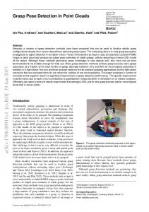
Our method, on the other hand, solve or partially solve the above problems and thus get a superior performance in this challenging dataset. Figure 8 shows the pole detection and classification result of the whole area and Figure 10 shows some close-ups. The time complexity is generally linear to the number of points in data in segmentation, and most computation needs to be done only on the segmented candidates. The overall running time is around 3 hours, which is fast and demonstrates the feasibility of our method for large-scale urban data. Figure 9 shows the typical failure cases of our method: trees with small crown could be easily confused with the lights with many bulbs. This could possibly be solved by taking more contextual information into account, which is part of our future work. VIII. C ONCLUSION AND F UTURE W ORK In this work, we propose an efficient and easy-toimplement algorithm for pole detection from the 3D scanned point cloud of the urban area. We introduce a series of slicing, combination and filtering strategies, and propose a five-class point classification method to help validate as well
Fig. 8.
Pole detection and classification result of the whole area.
(a)
(b)
Fig. 9. Typical failure cases of our method. The left is a false alarm due to the sparsity of the tree, while the right is a false negative caused by a light with many bulbs.
(a)
as classify the poles. There are some possible improvements in the future work. For example, a plane removal step could be incorporated in pre-processing. Moreover, as indicated in the failure case analysis, the contextual information could be beneficial for figuring out the outliers. Also, we are working on a pole classification method that can further classify the poles into more detailed subcategories. R EFERENCES [1] P. Doubek, M. Perdoch, J. Matas, and J. Sochman, “Mobile mapping of vertical traffic infrastructure,” in Proceedings of the 13th Computer Vision Winter Workshop, pp. 115–122, 2008. [2] D.-a. Luo and Y.-m. Wang, “Rapid extracting pillars by slicing point clouds,” in Proc. XXI ISPRS Congress, IAPRS, vol. 37, pp. 215–218, Citeseer, 2008. [3] S. Pu, M. Rutzinger, G. Vosselman, and S. Oude Elberink, “Recognizing basic structures from mobile laser scanning data for road inventory studies,” ISPRS Journal of Photogrammetry and Remote Sensing, vol. 66, no. 6, pp. S28–S39, 2011. [4] P. Press and D. Austin, “Approaches to pole detection using ranged laser data,” in Proceedings of Australasian Conference on Robotics and Automation, Citeseer, 2004. [5] T. Aschoff and H. Spiecker, “Algorithms for the automatic detection of trees in laser scanner data,” International Archives of Photogrammetry, Remote Sensing and Spatial Information Sciences, vol. 36, no. Part 8, p. W2, 2004. [6] H. Yokoyama, H. Date, S. Kanai, and H. Takeda, “Detection and classification of pole-like objects from mobile laser scanning data of urban environments,” International Journal of CAD/CAM, vol. 13, no. 2, 2013. [7] A. Golovinskiy, V. G. Kim, and T. Funkhouser, “Shape-based recognition of 3d point clouds in urban environments,” in Computer Vision, 2009 IEEE 12th International Conference on, pp. 2154–2161, IEEE, 2009. [8] F. Tombari, N. Fioraio, T. Cavallari, S. Salti, A. Petrelli, and L. Di Stefano, “Automatic detection of pole-like structures in 3d urban environments,” in Intelligent Robots and Systems (IROS 2014), 2014 IEEE/RSJ International Conference on, pp. 4922–4929, IEEE, 2014. [9] J.-F. Lalonde, N. Vandapel, D. F. Huber, and M. Hebert, “Natural terrain classification using three-dimensional ladar data for ground robot mobility,” Journal of field robotics, vol. 23, no. 10, pp. 839– 861, 2006. [10] J. Demantk´e, C. Mallet, N. David, and B. Vallet, “Dimensionality based scale selection in 3d lidar point clouds,” International Archives of Photogrammetry, Remote Sensing and Spatial Information Sciences, Laser Scanning, 2011. [11] J. Behley, K. Kersting, D. Schulz, V. Steinhage, and A. B. Cremers, “Learning to hash logistic regression for fast 3d scan point classification,” in Intelligent Robots and Systems (IROS), 2010 IEEE/RSJ International Conference on, pp. 5960–5965, IEEE, 2010. [12] O. Hadjiliadis and I. Stamos, “Sequential classification in point clouds of urban scenes,” in Proc. 3DPVT, 2010. [13] C.-C. Chang and C.-J. Lin, “Libsvm: a library for support vector machines,” ACM Transactions on Intelligent Systems and Technology (TIST), vol. 2, no. 3, p. 27, 2011.
(b)
(c)
(d) Fig. 10. Close-ups of pole detection and classification result by our method. We use yellow color to denote the lights, blue color to denote utility poles and red color to denote signs.